Abstract We obtain the large deviation functional of a density profile for the asymmetric exclusion process of $L$ sites with open boundary conditions when the asymmetry scales like $\frac{1}{L}$. We recover as limiting cases the expressions derived recently for the symmetric (SSEP) and the asymmetric (ASEP) cases. In the ASEP limit, the non linear differential equation one needs to solve can be analysed by a method which resembles the WKB method.

Key words: Large deviations, asymmetric simple exclusion process, open system, stationary non-equilibrium state.

1 Introduction

The study of steady states of non-equilibrium systems has motivated a lot of works over the last decades [1, 2, 3, 4, 5, 6, 7, 8, 9]. It is now well established that non-equilibrium systems exhibit in general long-range correlations in their steady state [4, 10, 11, 12].

One of the most studied examples of non-equilibrium system is the one dimensional exclusion process with open boundaries [4, 10, 13]. The system is a one dimensional lattice gas on a lattice of $L$ sites. At any given time, each site ($1\leq i\leq L$) is either empty or occupied by at most one particle and the system evolves according to the following rule: in the interior of the system ($2\leq i\leq L-1$), during each infinitesimal time interval $dt$, a particle attempts to jump to its right neighboring site with probability $dt$ and to its left neighboring site with probability $q\ dt$. The jump is completed if the target site is empty, otherwise nothing happens. The parameter $q$ represents a bias (i.e. the effect of an external field in the bulk). The boundary sites $i=1$ and $i=L$ are connected to reservoirs of particles and their dynamics is modified as follows: if site 1 is empty, it becomes occupied with probability $\alpha\ dt$ by a particle from the left reservoir, and if it is occupied, the particle is removed with a probability $\gamma\ dt$ or attempts to jump to site 2 (succeeding if this site is empty) with probability $dt$. Similarly, if site $L$ is occupied, the particle may either jump out of the system (into the right reservoir) with probability $\beta\ dt$ or to site $L-1$ with probability $q\ dt$, and if it is empty, it becomes occupied with probability $\delta\ dt$.

The rates $\alpha$, $\beta$, $\gamma$ and $\delta$ at which particles are injected at sites $1$ and $L$ can be thought as the contact of the chain with a reservoir of particles at density $\rho_{a}$ at site $1$ and with a reservoir at density $\rho_{b}$ at site $L$. The reservoir densities $\rho_{a}$ and $\rho_{b}$ are related to $\alpha$, $\beta$, $\gamma$ and $\delta$ by (see appendix)

$$\rho_{a} =\frac{1-q+\alpha+\gamma-\sqrt{(\alpha-\gamma-1+q)^{2}+4\alpha\gamma}}{2(1-q)}$$ (1.1a)

$$\rho_{b} =\frac{1-q-\beta-\delta+\sqrt{(\beta-\delta-1+q)^{2}+4\beta\delta}}{2(1-q)}$$ (1.1b)

For $q=1$, the bulk dynamics is symmetric and the model is called the Symmetric Simple Exclusion Process (SSEP) [2, 3]. In the steady state, there is a current of particles flowing from one reservoir to the other (when $\rho_{a}\neq\rho_{b}$) and the steady state density profile is linear.

For $0\leq q<1$, the bulk dynamics is asymmetric and the model is called the Asymmetric Simple Exclusion Process (ASEP) [14, 15, 16]. When the densities $\rho_{a}$ and $\rho_{b}$ vary, the system exhibits phase transitions, with different phases: a low density phase, a high density phase and a maximal current phase [16, 17, 18, 19]. On a macroscopic scale, the steady state profile is constant except along the first order transition line $\rho_{a}=\rho_{b}<1/2$ separating the low and the high density phases.

In the large $L$ limit, the probability $P_{L}\big{(}\{\rho(x)\}\big{)}$ of observing a given macroscopic density profile $\rho(x)$, $0\leq x\leq 1$ can be expressed through the large deviation functional ${\cal F}(\{\rho(x)\};\rho_{a},\rho_{b})$ by

$$P_{L}\big{(}\{\rho(x)\}\big{)} \sim e^{-L{\cal F}(\{\rho(x)\};\rho_{a},\rho_{b})}$$ (1.2)

This large deviation functional ${\cal F}$ is an extension of the notion of free energy to non-equilibrium systems [20, 21, 22].
One can think of a number of distinct definitions of $P_{L}\big{(}\{\rho(x)\}\big{)}$ which all lead to the same ${\cal F}$ in the large $L$ limit. Here, by dividing the system into $k$ boxes of size $L_{1}$, $L_{2}$,…, $L_{k}$ (with $\sum_{i=1}^{k}L_{i}=L$), we define $q_{L_{1},L_{2},\dots,L_{k}}(N_{1},N_{2},\dots,N_{k})$ as the probability of observing in the steady state $N_{1}$ particles in the first box, $N_{2}$ in the second, …, $N_{k}$ in the last box. Then if we identify $P_{L}(\{\rho(x)\})$ with $q_{L_{1},L_{2},\dots,L_{k}}(N_{1},N_{2},\dots,N_{k})$, one expects that for large $L$, (1.2) holds when $1\ll L_{i}\ll L$ and $N_{i}$ is the integer part of $L_{i}\rho(x_{i})$ where $x_{i}=\sum_{j=1}^{i}\frac{L_{j}}{L}$

In [20, 23, 21, 24, 25, 26], the following exact expressions of ${\cal F}(\{\rho(x)\};\rho_{a},\rho_{b})$ were obtained:

In the symmetric case, i.e. for $q=1$, it was shown in [20, 21] that

$${\cal F}_{\text{SSEP}}(\{\rho(x),\rho_{a},\rho_{b}\}) = \sup_{F(x)}\int_{0}^{1}dx\left\{\rho(x)\log\left(\frac{\rho(x)}{F(x)}\right)+(1-\rho(x))\log\left(\frac{1-\rho(x)}{1-F(x)}\right)\right.$$ (1.3)

$$\hskip 100.0pt+\left.\log\left(\frac{F^{\prime}(x)}{\rho_{b}-\rho_{a}}\right)\right\}.$$

where the $\sup$ is over all monotone functions $F(x)$ which satisfy

$$F(0)=\rho_{a}\;,\ \ \ \ \;\ \ \ \ F(1)=\rho_{b}\;.$$ (1.4)

The auxiliary function $F(x)$ which achieves the $\sup$ is the monotone solution of the nonlinear differential equation

$$\rho(x)=F(x)+\frac{F(x)(1-F(x))F^{\prime\prime}(x)}{F^{\prime}(x)^{2}}\;,$$ (1.5)

with the boundary conditions (1.4).

In the asymmetric case (i.e. for $q<1$), the expression of ${\cal F}(\{\rho(x)\};\rho_{a},\rho_{b})$ is given [25, 26]

• in the case $\rho_{a}\geq\rho_{b}$ by

  $${\cal F}_{\rm ASEP}(\{\rho(x)\};\rho_{a},\rho_{b})=-K(\rho_{a},\rho_{b})\hskip-190.0pt$$

  $$+ \sup_{F(x)}\int_{0}^{1}dx\,\rho(x)\log\left[\rho(x)(1-F(x))\right]+(1-\rho(x))\log\left[(1-\rho(x))F(x)\right],$$

  where the $\sup$ is over all monotone non-increasing functions $F(x)$ such that $F(0)=\rho_{a}$ and $F(1)=\rho_{b}$ and

  $$K(\rho_{a},\rho_{b})=\sup_{\rho_{b}\leq\rho\leq\rho_{a}}\log[\rho(1-\rho)],$$ (1.7)

  As shown in [26], the function $F(x)$ which gives the sup in (• ‣ 1) is the derivative of the concave envelope of $\int_{0}^{x}[1-\rho(x^{\prime})]dx^{\prime}$, whenever this derivative belongs to $]\rho_{b},\rho_{a}[$, and it takes the value $\rho_{a}$ or $\rho_{b}$ otherwise. As a result, when $F(x)$ differs from $\rho_{a}$ and $\rho_{b}$, it is made up of a succession of domains where $F(x)=1-\rho(x)$ and of domains where $F(x)$ is constant (as $F(x)$ is decreasing, it cannot in general coincide with $1-\rho(x)$ everywhere). In the domains where $F(x)$ is constant (and differs from $\rho_{a}$ and $\rho_{b}$) it satisfies a Maxwell construction rule: when $F(x)=C$ for $0<t\leq x\leq u<1$, its value is determined by

  $$(u-t)C =\int_{t}^{u}\big{[}1-\rho(x)\big{]}\,dx$$ (1.8)

• and in the case $\rho_{a}\leq\rho_{b}$ by
  

  $${\cal F}_{\rm ASEP}(\{\rho(x)\};\rho_{a},\rho_{b}))=-K(\rho_{a},\rho_{b})+\hskip 100.0pt$$ (1.9)

  $$\inf_{0\leq y\leq 1}\left\{\int_{a}^{y}dx\,\rho(x)\log\left[{\rho(x)(1-\rho_{a})}\right]+(1-\rho(x))\log\left[(1-\rho(x))\rho_{a}\right]\right.$$

  $$\left.+\int_{y}^{b}dx\,\rho(x)\log\left[\rho(x)(1-\rho_{b})\right]+(1-\rho(x))\log\left[(1-\rho(x))\rho_{b}\right]\right\}.$$

  where

  $$K(\rho_{a},\rho_{b})=\min\left[\log\rho_{a}(1-\rho_{a}),\log\rho_{b}(1-\rho_{b})\right],$$ (1.10)

The goal of the present paper is to reconcile the expression valid in the symmetric case (1.3) with those valid in the asymmetric case (• ‣ 1,1.9) by calculating the large deviation functional in a weak asymmetry regime, which interpolates between the two, where $q\to 1$ as $L\to\infty$ with $q=1-\frac{\lambda}{L}$. The SSEP and the ASEP appear therefore as limiting cases of the results obtained in the present paper.

The outline of the paper is as follows: in section 2, we summarize our results by writing several equivalent expressions of ${\cal F}$ in the weak asymmetry regime. In section 3 we give the details of our derivation. In section 4, we show how the SSEP and the ASEP expressions can be recovered in the limit $\lambda\to 0$ and $\lambda\to\infty$. The large $\lambda$ limit is somewhat reminiscent of the WKB method and the calculation of the position (1.8) of the plateaux in the Maxwell construction of the function $F(x)$ have an origin very similar to the Bohr-Sommerfeld rule in the WKB method [27, 28]. In section 5 we extend the range of validity of our results and show in particular that they remain true when detailed balance is verified.

2 Main results

We consider here a weak asymmetry regime defined as a situation where $q\to 1$ as $L\to\infty$,

$$q =1-\frac{\lambda}{L}$$ (2.11)

keeping $\lambda$ fixed.

For technical reasons which will become clear at the end of section 3.3, our results are limited to the case

$$\lambda >0 \rho_{a} >\rho_{b}$$ and (2.12)

In section 5, we will discuss some extensions to a broader range of parameters.

Our main result is that in the weak asymmetry regime, the large deviation functional is given by

$${\cal F}(\{\rho(x)\};\rho_{a},\rho_{b})=-K_{\lambda}(\rho_{a},\rho_{b})+\inf\limits_{\{y(x)\}}\left\{\vphantom{-y(0)\log\frac{1-\rho_{a}}{\rho_{a}}-y(1)\log\frac{\rho_{b}}{1-\rho_{b}}+\int_{0}^{1}dx\left[-\log\frac{\left|1-e^{-\lambda y}\right|}{\lambda}+\rho\log\rho+(1-\rho)\log{(1-\rho)}+(1-\rho+y^{\prime})\log{(1-\rho+y^{\prime})}+(\rho-y^{\prime})\log{(\rho-y^{\prime})}\right]}y(0)\log\frac{\rho_{a}}{1-\rho_{a}}+y(1)\log\frac{1-\rho_{b}}{\rho_{b}}\right.\\ +\int_{0}^{1}dx\left[-\log\frac{1-e^{-\lambda y}}{\lambda}+\rho\log\rho+(1-\rho)\log{(1-\rho)}\vphantom{-\log\frac{1-e^{-\lambda y}}{\lambda}+\rho\log\rho+(1-\rho)\log{(1-\rho)}+(1-\rho+y^{\prime})\log{(1-\rho+y^{\prime})}+(\rho-y^{\prime})\log{(\rho-y^{\prime})}}\right.\\ \left.\left.\vphantom{-\log\frac{1-e^{-\lambda y}}{\lambda}+\rho\log\rho+(1-\rho)\log{(1-\rho)}+(1-\rho+y^{\prime})\log{(1-\rho+y^{\prime})}+(\rho-y^{\prime})\log{(\rho-y^{\prime})}}+(1-\rho+y^{\prime})\log{(1-\rho+y^{\prime})}+(\rho-y^{\prime})\log{(\rho-y^{\prime})}\right]\vphantom{-y(0)\log\frac{1-\rho_{a}}{\rho_{a}}-y(1)\log\frac{\rho_{b}}{1-\rho_{b}}+\int_{0}^{1}dx\left[-\log\frac{1-e^{-\lambda y}}{\lambda}+\rho\log\rho+(1-\rho)\log{(1-\rho)}+(1-\rho+y^{\prime})\log{(1-\rho+y^{\prime})}+(\rho-y^{\prime})\log{(\rho-y^{\prime})}\right]}\right\}$$ (2.13)

where the $\inf$ is over all continuous positive functions $y(x)$ satisfying

$$\rho(x)-1\leq y^{\prime}(x)\leq\rho(x)\ \ .$$

We will show at the end of section 3.5 that the constant $K_{\lambda}(\rho_{a},\rho_{b})$ is given by

$$K_{\lambda}(\rho_{a},\rho_{b}) =\log(J)-\int_{\rho_{b}}^{\rho_{a}}\frac{d\rho}{\lambda\rho(1-\rho)}\log\left(1-\frac{\lambda\rho(1-\rho)}{J}\right)$$ (2.14)

where the parameter $J$ is solution of

$$\int_{\rho_{b}}^{\rho_{a}}\frac{d\rho}{J-\lambda\rho(1-\rho)} =1\ \ \ .$$ (2.15)

The parameter $J$ is in fact related to the steady state current $j$ by (see section 3.5)

$$J =\lim_{L\rightarrow\infty}Lj$$ (2.16)

Expression (2.13) for ${\cal F}$ can be rewritten in a form which interpolates between the symmetric (1.3) and the asymmetric (• ‣ 1) cases (see section 3.4):

$${\cal F}(\{\rho(x)\};\rho_{a},\rho_{b})=-K_{\lambda}(\rho_{a},\rho_{b})+\int_{0}^{1}dx\left\{\vphantom{\rho\log\frac{\rho}{F}+(1-\rho)\log\frac{1-\rho}{1-F}+\log(|F(1-F)\lambda-F^{\prime}|)+\frac{F^{\prime}}{\lambda F(1-F)}\log\left(-\frac{F^{\prime}}{F(1-F)\lambda-F^{\prime}}\right)}\rho\log{\frac{\rho}{F}}+(1-\rho)\log\frac{1-\rho}{1-F}\right.\\ \left.\vphantom{\rho\log\frac{\rho}{F}+(1-\rho)\log\frac{1-\rho}{1-F}+\log(F(1-F)\lambda-F^{\prime})+\frac{F^{\prime}}{\lambda F(1-F)}\log\left(-\frac{F^{\prime}}{F(1-F)\lambda-F^{\prime}}\right)}+\log{(F(1-F)\lambda-F^{\prime})}+\frac{F^{\prime}}{\lambda F(1-F)}\log{\left(-\frac{F^{\prime}}{F(1-F)\lambda-F^{\prime}}\right)}\right\}$$ (2.17)

where the function $F(x)$ is the solution of the differential equation

$$(F-\rho){F^{\prime}}^{2}+F(1-F)F^{\prime\prime}+\lambda F(1-F)(F-1+\rho)F^{\prime}=0$$ (2.18)

with the boundary conditions

$$F(0) =\rho_{a} F(1) =\rho_{b}$$ (2.19)

In the range of validity of our derivation (2.12) this differential equation has a unique solution, and this solution is monotone (see section 3.4).
Actually, if we consider the right hand side of (2.17) as a functional of function $F$, then (2.18) appears to be the condition that $F$ maximizes this functional under the constraint (2.19) (see the end of section 3.4), leading to

$${\cal F}(\{\rho(x)\},\rho_{a},\rho_{b})=\sup_{F}\left[-K_{\lambda}(\rho_{a},\rho_{b})+\int_{0}^{1}dx\left\{\vphantom{\rho\log\frac{\rho}{F}+(1-\rho)\log\frac{1-\rho}{1-F}+\log(|F(1-F)\lambda-F^{\prime}|)+\frac{F^{\prime}}{\lambda F(1-F)}\log\left(-\frac{F^{\prime}}{F(1-F)\lambda-F^{\prime}}\right)}\rho\log{\frac{\rho}{F}}+(1-\rho)\log\frac{1-\rho}{1-F}\right.\right.\\ \left.\left.\vphantom{\rho\log\frac{\rho}{F}+(1-\rho)\log\frac{1-\rho}{1-F}+\log(F(1-F)\lambda-F^{\prime})+\frac{F^{\prime}}{\lambda F(1-F)}\log\left(-\frac{F^{\prime}}{F(1-F)\lambda-F^{\prime}}\right)}+\log{(F(1-F)\lambda-F^{\prime})}+\frac{F^{\prime}}{\lambda F(1-F)}\log{\left(-\frac{F^{\prime}}{F(1-F)\lambda-F^{\prime}}\right)}\right\}\right]$$ (2.20)

where the $\sup$ is over all decreasing functions $F$ satisfying (2.19).

As ${\cal F}$ is a $\sup$ over convex functions of $\rho$, it is a convex function of $\rho$ in domain (2.12).

A by-product of (2.17) is (see section 3.5) that the most likely profile $\bar{\rho}(x)$ is solution of

$$\int_{\bar{\rho}(x)}^{\rho_{a}}\frac{d\rho}{J-\lambda\rho(1-\rho)} =x\ \ \ .$$ (2.21)

Depending on the boundary conditions this leads either to a $\tan$ profile, a $\tanh$ profile, or a $\coth$ profile.

3 Derivation

3.1 The matrix method

The equal time steady state properties of the ASEP can be exactly calculated using the so-called matrix method [14]. Let us consider a microscopic configuration defined by its occupation number $\{\tau_{i}\}$ where $\tau_{i}=1$ when site $i$ is occupied by a particle, and $0$ otherwise. It can be shown that the steady state probability of such a configuration for a lattice of $L$ sites can be written as

$$P(\{\tau_{i}\}) =\frac{\langle W|\prod_{i=1}^{L}(\mathbf{D}\tau_{i}+\mathbf{E}(1-\tau_{i}))|V\rangle}{Z_{L}(q)}$$ (3.22)

with $Z_{L}(q)$ being a normalization factor defined by

$$Z_{L}(q) =\langle W|(\mathbf{D}+\mathbf{E})^{L}|V\rangle$$ (3.23)

where $\mathbf{D}$ and $\mathbf{E}$ are two operators fulfilling the followings algebraic rules:

$$\mathbf{D}\mathbf{E}-q\mathbf{E}\mathbf{D} =\mathbf{D}+\mathbf{E}\;,$$ (3.24a)

$$\{\beta\mathbf{D}-\delta\mathbf{E}\}|V\rangle =|V\rangle\;,$$ (3.24b)

$$\langle W|\{\alpha\mathbf{E}-\gamma\mathbf{D}\} =\langle W|\;.$$ (3.24c)

These rules (3.24a)-(3.24c) allow the computation of all equal time steady state properties without the need of finding an explicit representation.

The two point correlation function $<\tau_{i}\tau_{j}>$ (where the symbol $<.>$ stands for the average with respect to the steady state probability) is given by

$$<\tau_{i}\tau_{j}> =\frac{\langle W|(D+E)^{i-1}D(D+E)^{j-i-1}D(D+E)^{L-j}|V\rangle}{Z_{L}(q)}$$ (3.25)

and the steady state current $j$ between site $i$ and $i+1$ is given by:

$$j =<\tau_{i}(1-\tau_{i+1})>-q<(1-\tau_{i})\tau_{i+1}>$$ (3.26)

Using expression (3.25) for the correlation function and the algebra rule (3.24a), one gets

$$j =\frac{Z_{L-1}(q)}{Z_{L}(q)}\ \ \ .$$ (3.27)

Clearly the current does not depend on the site $i$, as it should, due to the conservation of the number of particles.

If we divide the system of size $L$ in $k$ boxes of size $L_{1}$, $L_{2}$, …$L_{k}$ the probability of finding $N_{1}$ particles in the first box, $N_{2}$ in the second, …and $N_{k}$ in the last box is given by

$$q_{L_{1},L_{2},\cdots L_{k}}(N_{1},N_{2},\cdots,N_{k}) =\frac{\langle W|X_{L_{1}}(N_{1})X_{L_{2}}(N_{2})\cdots X_{L_{k}}(N_{k})|V\rangle}{Z_{L}(q)}$$ (3.28)

where $X_{l}(N)$ is the sum over all products of $l$ matrices containing exactly $N$ matrices $\mathbf{D}$ and $l-N$ matrices $\mathbf{E}$.

3.2 A representation for $\mathbf{D}$ and $\mathbf{E}$

All physical quantities such as (3.25), (3.26) or (3.28) do not depend on the representation of the matrices $\mathbf{D}$ and $\mathbf{E}$ and of the vectors $|V\rangle$ and $\langle W|$ which satisfy the algebra (3.24a)-(3.24c). Several representations have been used to solve (3.24a-3.24c) [17, 15, 16, 29, 14]. We choose in this section a particular representation which will be convenient for the remaining of our derivation.

If we write the operators $\mathbf{D}$ and $\mathbf{E}$ as infinite matrices of the form

$$\mathbf{D} =\frac{1}{1-q}\left[\begin{array}[]{c c c c c}1-d&1-q&0&&\cdots\\ 0&1-dq&1-q^{2}&0&\cdots\\ 0&0&1-dq^{2}&1-q^{3}&0\\ &\ddots&\ddots&\ddots&\ddots\end{array}\right],$$ (3.29e)

$$\mathbf{E} =\frac{1}{1-q}\left[\begin{array}[]{c c c c c }1-e&0&0&0&\cdots\\ 1-ed&1-eq&0&0&\cdots\\ 0&1-edq&1-eq^{2}&0&\cdots\\ 0&\ddots&\ddots&\ddots&\ddots\end{array}\right],$$ (3.29j)

we find that they satisfy the algebraic rule (3.24a) for arbitrary choices of $d$ and $e$.

Let call $\{|n\rangle\}_{n\geq 1}$ the vector of the associated basis. If we look for vectors $|V\rangle$ and $\langle W|$ of the form

$$\langle W| =\sum_{n=1}^{\infty}\left(\frac{1-\rho_{a}}{\rho_{a}}\right)^{n}\langle n|$$ (3.30a)

$$|V\rangle =\sum_{n=1}^{\infty}\left(\frac{\rho_{b}}{1-\rho_{b}}\right)^{n}\frac{(ed;q)_{n-1}}{(q;q)_{n-1}}|n\rangle$$ (3.30b)

where $\rho_{a}$ and $\rho_{b}$ are for the moment arbitrary and the symbol $(x;q)_{i}$ stands for the $q$-shifted factorial defined by $(x;q)_{0}=1$ and

$$(x;q)_{i} =\prod_{k=0}^{i-1}(1-xq^{k}) \text{for }k >0\ \ \$$ (3.31a)

one can check that (3.30a) and (3.30b) fulfill the algebraic rules (3.24b) and (3.24c) if the parameters $\rho_{a}$, $\rho_{b}$, $d$ and $e$ satisfy:

$$\frac{\alpha}{\rho_{a}}-\frac{\gamma}{1-\rho_{a}} =1-q$$ (3.32a)

$$\frac{\beta}{1-\rho_{b}}-\frac{\delta}{\rho_{b}} =1-q$$ (3.32b)

$$d =\frac{\delta(1-\rho_{b})}{\beta\rho_{b}}$$ (3.32c)

and

$$e =\frac{\gamma\rho_{a}}{\alpha(1-\rho_{a})}$$ (3.32d)

Note that the parameters $\rho_{a}$ and $\rho_{b}$ defined by (1.1a) and (1.1b), that we interpreted as the reservoir densities, are the unique solutions of the equations (3.32a) and (3.32b) such that $0\leq\rho_{a}\leq 1$ and $0\leq\rho_{b}\leq 1$ (this is why we use the same symbol in (3.9) and (1.1)).

If we use this representation when $q<1$ (which is not a restriction due to the left-right symmetry), we see that the condition for $\langle W|X|V\rangle$ to be finite when $X$ is an arbitrary product of $\mathbf{D}$ and $\mathbf{E}$ is that $\rho_{a}>\rho_{b}$, leading to (2.12). In section 5, we will show that this representation remains valid for some part of the domain $q>1$, thus allowing us to extend the result of section 2 .

3.3 The sum over paths and the derivation of (2.13)

The basic idea of our derivation of (2.13) is to expand the matrix products such as (3.22) or (3.28) as a sum over paths [12], in much the same way as the path integral formulation of quantum mechanics.

Consider the set of discrete walks $w$ of $k$ steps. Let $n_{i}(w)$ ($0\leq i\leq k$) be the integer position of the walk after the $i$th step. The walks we consider remain positive $n_{i}>0$ and their increment at each step satisfies

$$n_{i} >0 -L_{i}\leq n_{i}-n_{i-1}\leq L_{i}$$ and (3.33)

From (3.28), we deduce

$$q_{L_{1},L_{2},\cdots L_{k}}\big{(}N_{1},N_{2},\cdots,N_{k}\big{)} =\frac{1}{Z_{L}(q)}\sum_{w}\langle W|n_{0}\rangle\langle n_{k}|V\rangle\prod_{i=1}^{k}\langle n_{i-1}|X_{L_{i}}(N_{i})|n_{i}\rangle$$ (3.34)

where $X_{l}(N)$ has been defined in (3.28).

In the large $L$ limit (with $q=1-\frac{\lambda}{L}$), (1.1a) and (1.1b) become

$$\rho_{a} =\frac{\alpha}{\alpha+\gamma}+O(\frac{1}{L}) \rho_{b} =\frac{\delta}{\beta+\delta}+O(\frac{1}{L})$$ (3.35)

and (3.32d), (3.32c)

$$d =1+O(\frac{1}{L}) e =1+O(\frac{1}{L})\ \ ,$$ (3.36)

To compute (3.34) when $1\ll L_{i}\ll L$, let us evaluate $\langle n|X_{l}(N)|n^{\prime}\rangle$ when $1\ll l\ll L$. When $n$, $n^{\prime}$ are of order $L$ with $|n-n^{\prime}|\leq l\ll L$, we see that for $m$ and $m^{\prime}$ in $(\min(n,n^{\prime})-l,\max(n,n^{\prime})+l)$ all the non-zero elements of matrix $\langle m|\mathbf{D}|m^{\prime}\rangle$ and $\langle m^{\prime}|\mathbf{E}|m\rangle$ are equivalent to

$$\langle m|\mathbf{D}|m^{\prime}\rangle\sim\langle m^{\prime}|\mathbf{E}|m\rangle\sim\left(1-e^{-\frac{\lambda n}{L}}\right)\frac{L}{\lambda}\ \ \ .$$ (3.37)

The computation of $\langle n|X_{l}(N)|n^{\prime}\rangle$ is thus reduced to an enumeration problem. This leads to

$$\langle n|X_{l}(N)|n^{\prime}\rangle \simeq\left[\left(1-e^{-\frac{\lambda n}{L}}\right)\frac{L}{\lambda}\right]^{l}\sum_{n_{+}-n_{-}=n^{\prime}-n}\binom{l}{N}\binom{N}{n_{+}}\binom{l-N}{n_{-}}$$ (3.38)

where $\binom{l}{N}$ is the number of words of length $l$ with $N$ matrices $\mathbf{D}$ and $l-N$ matrices $\mathbf{E}$, $n_{+}$ is the number of matrix elements of the form $\langle m|\mathbf{D}|m+1\rangle$ and $n_{-}$ the number of matrix elements of the form $\langle m|\mathbf{E}|m-1\rangle$.
Looking at the values of $n_{+}$ and $n_{-}$ which dominate (3.38) one obtains

$$\log\langle n|X_{l}(N)|n^{\prime}\rangle=l\left[-\log\frac{\lambda}{L}+\log\left(1-e^{-\lambda y}\right)-\rho\log\rho-(1-\rho)\log(1-\rho)\vphantom{\left(1-y^{\prime}\right)\log\left({1-y^{\prime}}\right)}\right.\\ -\left(1-\rho+y^{\prime}\right)\log\left(1-\rho+y^{\prime}\right)\left.-\left(\rho-y^{\prime}\right)\log\left(\rho-y^{\prime}\right)\vphantom{log\left(1-e^{-(\lambda y)}\right)}+o(1)\right]$$ (3.39)

where $y$, $y^{\prime}$ and $\rho$ are defined by

$$y =\frac{n}{L} y^{\prime} =\frac{n^{\prime}-n}{l} \rho=\frac{N}{l}\ \ .$$ and (3.40)

As $\frac{L_{i}}{L}\to 0$ while $L_{i}\to\infty$, one can associate to each walk $w$ a continuous function $y(x)$

$$y\left(x_{i}\right) =\frac{n_{i}(w)}{L}$$ (3.41)

with $x_{i}=\sum_{j=1}^{i}\frac{L_{j}}{L}$. For each walk $y(x)$ and each density profile $\rho(x)$ such that

$$y(x) >0 \rho(x)-1 \leq y^{\prime}(x)\leq\rho(x)$$ and (3.42)

(these restrictions on the path $y$ come from $n_{i}(w)>0$ (see (3.33)) and the condition for $\langle n|X_{l}(N)|n^{\prime}\rangle\neq 0$ (see (3.39))), let us define ${\cal G}\big{(}\{y(x)\},\{\rho(x)\}\big{)}$ by

$${\cal G}\big{(}\{y(x)\},\{\rho(x)\}\big{)}=y(0)\log\frac{\rho_{a}}{1-\rho_{a}}+y(1)\log\frac{1-\rho_{b}}{\rho_{b}}+\\ \int_{0}^{1}dx\left[-\log\frac{1-e^{-\lambda y}}{\lambda}+\rho\log\rho+(1-\rho)\log{(1-\rho)}\vphantom{-\log\frac{1-e^{-\lambda y}}{\lambda}+\rho\log\rho+(1-\rho)\log{(1-\rho)}+(1-\rho+y^{\prime})\log{(1-\rho+y^{\prime})}+(\rho-y^{\prime})\log{(\rho-y^{\prime})}}\right.\\ \left.\vphantom{-\log\frac{1-e^{-\lambda y}}{\lambda}+\rho\log\rho+(1-\rho)\log{(1-\rho)}+(1-\rho+y^{\prime})\log{(1-\rho+y^{\prime})}+(\rho-y^{\prime})\log{(\rho-y^{\prime})}}+(1-\rho+y^{\prime})\log{(1-\rho+y^{\prime})}+(\rho-y^{\prime})\log{(\rho-y^{\prime})}\right]\ \ .$$ (3.43)

Then expression (3.34) leads to (after replacing the sum over $w$ by a sup over $w$)

$$\log q_{L_{1},L_{2},\cdots L_{k}}\big{(}N_{1},N_{2},\cdots,N_{k}\big{)} \simeq\log P_{L}\left(\{\rho(x)\}\right)$$ (3.44)

$$\simeq L\sup_{y}\big{[}K_{\lambda}(\rho_{a},\rho_{b})-{\cal G}\big{(}\{y(x)\},\{\rho(x)\}\big{)}\big{]}$$ (3.45)

with $K_{\lambda}(\rho_{a},\rho_{b})$ given by

$$K_{\lambda}(\rho_{a},\rho_{b}) =\lim_{L\rightarrow\infty}\left(\log L-\frac{\log Z_{L}(1-\frac{\lambda}{L})}{L}\right)\ \ .$$ (3.46)

which is the expression (2.13).

In order to compute $K_{\lambda}(\rho_{a},\rho_{b})$, we could use a similar method to estimate $Z_{L}(q)$ in (3.46); we will rather use the property that the most likely profile $\bar{\rho}$ must verify ${\cal F}(\{\bar{\rho}(x)\};\rho_{a},\rho_{b})=0$, so we delay the computation of $K_{\lambda}(\rho_{a},\rho_{b})$ until the end of section 3.5. Of course both methods give the same result.

3.4 Derivation of (2.17)

As the functions $-\log(1-e^{-\lambda y(x)})$, $\left(\rho(x)-y^{\prime}(x)\right)\log\left(\rho(x)-y^{\prime}(x)\right)$ and $\left(1-\rho(x)+y^{\prime}(x)\right)\log\left(1-\rho(x)+y^{\prime}(x)\right)$ are convex functions of $y$ for every value of $x$ , the function ${\cal G}\big{(}\{y(x)\},\{\rho(x)\}\big{)}$ in (3.43) is a sum of convex functions, and is thus convex.
Therefore there is a unique walk $y_{\text{m}}(x)$ which minimizes ${\cal G}\big{(}\{y(x)\},\{\rho(x)\}\big{)}$, so

$${\cal F}\left(\{\rho(x)\};\rho_{a},\rho_{b}\right) ={\cal G}\big{(}\{y_{\text{m}}(x)\},\{\rho\}\big{)}-K_{\lambda}(\rho_{a},\rho_{b})$$ (3.47)

This minimum is not reached at the boundary of (3.42). Thus $y_{\text{m}}(x)$ is the unique stationary point, solution of $\left.\frac{\partial{\cal G}\big{(}\{y\},\{\rho\}\big{)}}{\partial y(x)}\right|_{y=y_{\text{m}}}=0$ and it satisfies:

$$\frac{\rho^{\prime}(x)-y_{\text{m}}^{\prime\prime}(x)}{(1-\rho(x)+y_{\text{m}}^{\prime}(x))(\rho(x)-y_{\text{m}}^{\prime}(x))}-\lambda\frac{e^{-\lambda y_{\text{m}}(x)}}{1-e^{-\lambda y_{\text{m}}(x)}} =0$$ (3.48)

with the boundary conditions

$$1-\rho(0)+y_{\text{m}}^{\prime}(0) =\rho_{a} 1-\rho(1)+y_{\text{m}}^{\prime}(1) =\rho_{b}$$ (3.49)

in addition to the general condition (3.42).

To obtain an expression similar to (1.3), we rewrite (3.48) using the function $F(x)$ defined by

$$F(x) =1-\rho(x)+y_{\text{m}}^{\prime}(x)\ \ .$$ (3.50)

This lead to

$$\frac{F^{\prime}(x)}{F(x)(1-F(x))} =-\lambda\frac{e^{-\lambda y_{\text{m}}(x)}}{1-e^{-\lambda y_{\text{m}}(x)}}$$ (3.51)

with the boundary conditions

$$F(0) =\rho_{a} F(1) =\rho_{b}$$ (3.52)

The conditions on the walk (3.42) imply

$$0\leq F(x)\leq 1$$ (3.53)

and as $y>0$ (see (3.42) and (3.51))

$$F^{\prime}(x)<0$$ (3.54)

By eliminating $y$ between (3.50) and (3.51) we get (2.18).

The expression of the large deviation functional can be rewritten in terms of $F$ instead of $y_{\text{m}}$ in (2.13). From (3.51), we see that

$$\log\left(1-e^{-\lambda y_{\text{m}}}\right) =\log\frac{\lambda F(1-F)}{\lambda F(1-F)-F^{\prime}}$$ (3.55)

If we integrate by part the term $\int_{0}^{1}dxy^{\prime}(x)\log\frac{1-\rho(x)+y^{\prime}(x)}{\rho(x)-y^{\prime}(x)}$ in (2.13), we get

$$\int_{0}^{1}dx\,y^{\prime}\log\frac{1-\rho+y^{\prime}}{\rho-y^{\prime}} =\left[y\log\frac{1-\rho+y^{\prime}}{\rho-y^{\prime}}\right]_{0}^{1}$$

$$\ \ \ \ \ +\int_{0}^{1}dx\frac{y(\rho^{\prime}-y^{\prime\prime})}{(1-\rho+y^{\prime})(\rho-y^{\prime})}$$ (3.56)

$$=y(1)\log\frac{\rho_{b}}{1-\rho_{b}}-y(0)\log\frac{\rho_{a}}{1-\rho_{a}}$$

$$\ \ \ \ \ +\int_{0}^{1}\frac{F^{\prime}}{\lambda F(1-F)}\log\frac{-F^{\prime}}{\lambda F(1-F)-F^{\prime}}$$ (3.57)

and thus (2.13) leads to (2.17).

Let us now justify (2.20). If we define

$${\cal H}\left(\vphantom{\big{(}}\{\rho\},\{\phi\}\right)=-K_{\lambda}(\rho_{a},\rho_{b})+\int_{0}^{1}\left\{\rho(x)\log\rho(x)+\big{(}1-\rho(x)\big{)}\log\big{(}1-\rho(x)\big{)}\vphantom{\left(1-\frac{\phi^{\prime}(x)}{\lambda}\right)\log(\lambda-\phi^{\prime}(x))}\right.\\ +\big{(}1-\rho(x)\big{)}\phi(x)-\log\left(1+e^{\phi(x)}\right)\\ \left.+\frac{\phi^{\prime}(x)}{\lambda}\log\big{(}-\phi^{\prime}(x)\big{)}+\left(1-\frac{\phi^{\prime}(x)}{\lambda}\right)\log\big{(}\lambda-\phi^{\prime}(x)\big{)}\right\}\ \ ,$$ (3.58)

expression (2.17) implies that when $F$ is solution of (2.18) with condition (2.19) then

$${\cal F}\big{(}\{\rho\};\rho_{a},\rho_{b}\big{)} ={\cal H}\left(\vphantom{\big{(}}\{\rho\},\left\{\log\left(\frac{F}{1-F}\right)\right\}\right)$$ (3.59)

As $-\log(1+e^{\phi(x)})$ and $\frac{\phi^{\prime}(x)}{\lambda}\log\big{(}-\phi^{\prime}(x)\big{)}+\left(1-\frac{\phi^{\prime}(x)}{\lambda}\right)\log\big{(}\lambda-\phi^{\prime}(x)\big{)}$ are concave function of $\phi$ for $\phi^{\prime}<0$, ${\cal H}\left(\vphantom{\big{(}}\{\rho\},\{\phi\}\right)$ is a concave function of $\phi$. So (2.18) is equivalent to the condition for $F$ to maximize ${\cal H}\left(\vphantom{\big{(}}\{\rho\},\left\{\log\left(\frac{F}{1-F}\right)\right\}\right)$ under the constraint (2.19) and $F^{\prime}<0$, i.e.

$$\frac{\partial{\cal H}\left(\vphantom{\big{(}}\{\rho\},\left\{\log\left(\frac{F}{1-F}\right)\right\}\right)}{\partial F} =0\ \ .$$ (3.60)

So (3.59) can be written as

$${\cal F}\big{(}\{\rho(x)\};\rho_{a},\rho_{b}\big{)} =\sup_{F}\left[{\cal H}\left(\vphantom{\big{(}}\{\rho\},\left\{\log\left(\frac{F}{1-F}\right)\right\}\right)\right]$$ (3.61)

where the $\sup$ is taken over decreasing functions $F$ with the condition (2.19), leading to (2.20).

3.5 The most likely profile

From (2.20), we get

$$\frac{\partial{\cal F}(\{\rho(x)\};\rho_{a},\rho_{b})}{\partial\rho(x)} =\log\frac{\rho(1-F)}{(1-\rho)F}$$ (3.62)

so that for the most likely profile $\bar{\rho}(x)$

$$F(x) =\bar{\rho}(x)\ \ .$$ (3.63)

Equation (2.18) thus becomes

$$\bar{\rho}^{\prime\prime}=\lambda\bar{\rho}^{\prime}(1-2\bar{\rho})$$ (3.64)

with boundary conditions

$$\bar{\rho}(0) =\rho_{a} \bar{\rho}(1) =\rho_{b}$$ and (3.65)

Integrating (3.64) once, we get constant parameter $J$

$$\bar{\rho}^{\prime}=\lambda\bar{\rho}(1-\bar{\rho})-J$$ (3.66)

The boundary conditions (3.65) determine $J$ as given by equation (2.15) and $\bar{\rho}$ by (2.21).

One can show that (2.17) implies that

$$<\tau_{i}\tau_{i+1}> =<\tau_{i}><\tau_{i+1}>+O\left(\frac{1}{L}\right)$$ (3.67)

(see for example [23] for the case $\lambda=0$).
In particular $<\tau_{i}(1-\tau_{i+1})>\simeq<\tau_{i}><1-\tau_{i+1}>$ and (3.26) for $q=1-\frac{\lambda}{L}$ leads to

$$j =\frac{\lambda}{L}\bar{\rho}(1-\bar{\rho})-\frac{\bar{\rho}^{\prime}}{L}+o\left(\frac{1}{L}\right)\ \ .$$ (3.68)

Comparing (3.68) to (3.66) leads to relation (2.16) between $J$ and the current $j$.

Depending on the reservoir densities $\rho_{a}$ and $\rho_{b}$, one gets various expression for the most likely profile $\bar{\rho}(x)$

• when $\rho_{a}-\rho_{b}>\lambda\left(\rho_{a}-\frac{1}{2}\right)\left(\rho_{b}-\frac{1}{2}\right)$ then $J>\frac{\lambda}{4}$:

  $$\bar{\rho}(x) =\frac{1}{2}-\sqrt{\frac{J-\lambda/4}{\lambda}}\tan\left[\sqrt{\lambda(J-\lambda/4)}(x-x_{0})\right]$$ (3.69)

• and when $\rho_{a}-\rho_{b}<\lambda\left(\rho_{a}-\frac{1}{2}\right)\left(\rho_{b}-\frac{1}{2}\right)$ then $J<\frac{\lambda}{4}$ and

  $$\bar{\rho}(x) =\frac{1}{2}+\sqrt{\frac{\lambda/4-J}{\lambda}}\coth\left[\sqrt{\lambda(\lambda/4-J)}(x-x_{0})\right]$$ (3.70)

where $x_{0}$ and $J$ are chosen to satisfy (3.65).

Starting with the expression of the most likely profile, one can get an equation for $K_{\lambda}(\rho_{a},\rho_{b})$ by writing that

$${\cal F}(\{\bar{\rho}\};\rho_{a},\rho_{b})=0$$ (3.71)

Introducing equations (3.63) and (3.66) in expression (2.17) and solving (3.71) we get expression (2.14) for $K_{\lambda}(\rho_{a},\rho_{b})$.

4 Limiting cases

In this section we show how previously known expressions (1.3)-(1.7) can be recovered as limiting cases of the results (2.13-2.21) of the present paper.

4.1 The SSEP limit

Let us first consider the small $\lambda$ limit. Expression (2.15) for the current can be expanded in powers of $\lambda$.

$$j =\frac{\rho_{a}-\rho_{b}}{L}+\frac{\lambda}{L}\left(\frac{\rho_{a}+\rho_{b}}{2}-\frac{\rho_{a}^{2}+\rho_{a}\rho_{b}+\rho_{b}^{2}}{3}\right)+O(\lambda^{2})$$ (4.72)

in agreement (when $\lambda\to 0$) with $j=\frac{\rho_{a}-\rho_{b}}{L}$ of [3].
The large deviation functional (2.17) becomes for small $\lambda$

$${\cal F}=\int_{0}^{1}dx\left\{\rho\log\left(\frac{\rho}{F}\right)+(1-\rho)\log\left(\frac{1-\rho}{1-F}\right)\right.\\ \left.\vphantom{\rho\log\left(\frac{\rho}{F}\right)+(1-\rho)\log\left(\frac{1-\rho}{1-F}\right)}+\log(-F^{\prime})-\frac{\lambda F(1-F)}{2F^{\prime}}\right\}+1-K_{\lambda}(\rho_{a},\rho_{b})+O(\lambda^{2})\ \ .$$ (4.73)

The leading order in $\lambda$ agrees with the SSEP expression (1.3) as the constant $K_{\lambda}(\rho_{a},\rho_{b})$ given by (2.14) becomes

$$K_{\lambda}(\rho_{a},\rho_{b}) =\log(\rho_{a}-\rho_{b})+1+O(\lambda)$$ (4.74)

and the equation (1.5) for $F$ is the limiting case of (2.18) when $\lambda\to 0$. Furthermore one can check that the most likely profile (2.21) becomes linear as $J=Lj\to\rho_{a}-\rho_{b}$ in the small $\lambda$ limit. Thus the results known for SSEP are recovered from our general $\lambda$ case in the limit $\lambda\to 0$ .

4.2 The ASEP limit for $\rho_{a}>\rho_{b}$

Let us now see how the strongly asymmetric case (• ‣ 1) can be recovered from (2.17) for large $\lambda$. We see that for large $\lambda$, the solution $J$ of (2.15) is $J\simeq\max\limits_{\rho_{b}\leq\rho\leq\rho_{a}}\lambda\rho(1-\rho)$, so that

$$j \sim\sup\limits_{\rho_{b}\leq\rho\leq\rho_{a}}\frac{\lambda}{L}\rho(1-\rho) \rho_{a}>\rho_{b}$$ when (4.75)

in agreement with [18, 30], and that $K_{\lambda}(\rho_{a},\rho_{b})\simeq\log J$ in (2.14) so that (2.20) reduces to (• ‣ 1).

An interesting aspect of this large $\lambda$ limit is to see how the solution $F$ of (2.18) becomes for large $\lambda$ the function $F$ constructed from $1-\rho(x)$ by the Maxwell construction explained after equation (1.7). When $\lambda$ becomes large, (2.18) implies that $F\simeq 1-\rho$ or $F^{\prime}\simeq 0$. Therefore one expects a succession of domains where $F(x)\simeq 1-\rho(x)$ and domains where $F(x)$ is constant, with the remaining contraints that $F$ is monotone and $\rho_{b}\leq F(x)\leq\rho_{a}$

In a domain where $F(x)\simeq 1-\rho(x)$, one can expand $F$ in powers of $\frac{1}{\lambda}$

$$F =1-\rho+\frac{1}{\lambda}\left[\rho^{\prime}\frac{1-2\rho}{\rho(1-\rho)}-\frac{\rho^{\prime\prime}}{\rho^{\prime}}\right]+O\left(\frac{1}{\lambda^{2}}\right)\ \ \ .$$ (4.76)

The condition $F^{\prime}<0$ (3.54) implies that in such domains $\rho^{\prime}>0$

In a domain $t<x<u$ where $F(x)\simeq C$ is almost constant, neglecting ${F^{\prime}}^{2}$ in (2.18) (as ${F^{\prime}}^{2}\ll\lambda F^{\prime}$) gives

$$F^{\prime}(x) =B\exp{\left[-\lambda\int^{x}_{t}{(C-1+\rho(x^{\prime}))dx^{\prime}}\right]}$$ (4.77)

where $B$ is constant over the whole domain $t<x<u$.

The next question is to understand for large $\lambda$ the transitions between these different domains.

A first possibility is that $F(x)$ (which is monotone) becomes discontinuous at such transition point. This is the case for example when $1-\rho(x)$ is decreasing and discontinuous, implying that $F(x)$ has a variation of the order of $1$ (the discontinuity of $\rho$) over a range in $x$ of order of $\frac{1}{\lambda}$. This case can be analysed without difficulty, but we won’t discuss it here.

The other possibility is that for large $\lambda$, $F$ remains continuous but $F^{\prime}$ becomes discontinuous. This is what happens for example on figure 1: for large $\lambda$ there is a succession of domains where $F=1-\rho(x)$ and where $F$ is constant.

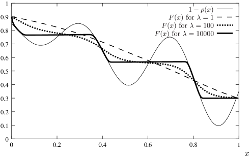
Figure 1: $F(x)$ solution of (2.18) versus $x$ for a given profile $\rho(x)$ and reservoir densities $\rho_{a}=0.9$, $\rho_{b}=0.3$ when $\lambda$ takes the value $1$, $100$ and $10000$. The full-curve is $1-\rho(x)$. The curves are obtained by minimizing (2.13) numerically for $y(x)$ (discretized over $200$ points). $F(x)$ is then calculated from $y(x)$ by relation (3.50). For large $\lambda$, we see a succession of domains where $F=1-\rho(x)$ and where $F$ is constant satisfying the Maxwell construction.

Let us consider a domain where $F(x)=1-\rho(t)=1-\rho(u)$ for $t<x<u$ in the large $\lambda$ limit, surrounded by two domains where $F(x)=1-\rho(x)$. At the transition point $t$, the solution of (2.18) takes a scaling form

$$F(x)-1+\rho(x) =\sqrt{\frac{\rho^{\prime}(t)}{\lambda}}G\big{(}(x-t)\sqrt{\rho^{\prime}(t)\lambda}\big{)}$$ (4.78)

where $G$ is solution of

$$G^{\prime\prime} =G(1-G^{\prime})$$ (4.79)

For $F$ to match the solution $1-\rho(x)+O(\frac{1}{\lambda})$ for $x=t-0$ and $1-\rho(t)+o(1)$ for $x=t+0$, one needs that

$$G(z) \rightarrow 0 z\rightarrow-\infty$$ when (4.80)

$$G(z) =z+o(1) z\rightarrow\infty$$ when (4.81)

It can be shown that then $G$ is solution of

$$G^{\prime} =1+W\left(Ae^{-\frac{G^{2}}{2}}\right)$$ (4.82)

where $W$ is the product logarithm function (also called the Lambert function, see [31]) defined here as the largest real solution of

$$W(x)e^{W(x)}=x$$ (4.83)

Condition (4.80) determines $A=-e^{-1}$ (as $W\left(-e^{-1}\right)=-1$). Using that for $x$ small $W(x)\simeq x$, the limit of $G$ for large $z$ can be computed

$$G(z)-z \sim\frac{1}{e}\int_{z}^{\infty}e^{-\frac{{z^{\prime}}^{2}}{2}}\,dz^{\prime}$$ (4.84)

It gives for the asymptotic regime (when $\frac{1}{\sqrt{\lambda}}\ll x-t\ll 1$) of $F^{\prime}$

$$F^{\prime}(x)\sim-\frac{\rho^{\prime}(t)}{e}e^{-\frac{\rho^{\prime}(t)\lambda}{2}(x-t)^{2}}$$ (4.85)

At the other boundary $u$ of the domain, $F$ has a similar scaling form.

$$F(x)-1+\rho(x) =-\sqrt{\frac{\rho^{\prime}(u)}{\lambda}}G\big{(}-(x-u)\sqrt{\rho^{\prime}(u)\lambda}\big{)}$$ (4.86)

with the same $G$ solution of (4.79). This gives for the asymptotic regime $\frac{1}{\sqrt{\lambda}}\ll-(x-u)\ll 1$

$$F^{\prime}(x)\simeq-\frac{\rho^{\prime}(u)}{e}e^{-\frac{\rho^{\prime}(u)\lambda}{2}(x-u)^{2}}$$ (4.87)

For the asymptotics of (4.77) to match with (4.85) as $x\to t$

$$F^{\prime}(x)\sim Be^{-\frac{\rho^{\prime}(t)\lambda}{2}(x-t)^{2}}$$ (4.88)

and with (4.87) when $x\to u$

$$F^{\prime}(x)\sim Be^{\left[-\lambda\int^{u}_{t}{(C-1+\rho(x^{\prime}))dx^{\prime}}\right]-\frac{\rho^{\prime}(u)\lambda}{2}(x-u)^{2}}$$ (4.89)

one needs that to the leading order in $\lambda$

$$\int^{u}_{t}(C-1+\rho(x^{\prime}))dx^{\prime} =0$$ (4.90)

which is the Maxwell construction (1.8). We see that the constant $C$, the value of $F(x)$ in a domain where $F$ is constant, is determined by an expression (4.90) which is obtained from two matching conditions at the boundaries of the domain. This is very similar to the Bohr Sommerfeld rule which determines the energy levels in the WKB method [27, 28]. So the Maxwell construction here has a mathematical origin similar to the Bohr Sommerfeld rule.

5 Extension of our results

5.1 Extension of the domain (2.12)

We are going to show that our results of section 2, initially derived in the domain (2.12) remain valid for

$$\lambda >0 e^{\lambda}\frac{1-\rho_{b}}{\rho_{b}}\frac{\rho_{a}}{1-\rho_{a}} <1$$ (5.91)

The representation of the algebra for $\mathbf{D}$, $\mathbf{E}$, $|V\rangle$ and $\langle W|$ introduced in section 3.2 remains valid for some range of the parameter $\rho_{a}$ and $\rho_{b}$ when $q>1$. Indeed, for large $n$ the non-zero matrix elements of the kind $\langle n|\mathbf{D}|n^{\prime}\rangle$ and $\langle n^{\prime}|\mathbf{E}|n\rangle$ behave then like $q^{n}$. Furthermore, $\frac{(ed;q)_{n}}{(q;q)_{n}}\sim\left(\frac{ed}{q}\right)^{n}$ for large $n$. Thus, using (3.32c) and (3.32d), we get that for any product $X$ of $L$ matrices $\mathbf{D}$ or $\mathbf{E}$ (and any sum of such product) $\langle W|n\rangle\langle n|X|V\rangle\sim\left(\frac{\gamma\delta}{\alpha\beta}q^{L-1}\right)^{n}$ and the condition for $\langle W|X|V\rangle$ to be finite is

$$\frac{\gamma\delta}{\alpha\beta}q^{L-1} <1\ \ .$$ (5.92)

When $q=1-\frac{\lambda}{L}$ and in the large $L$ limit, this leads to (using (3.35) )

$$\lambda <0 e^{-\lambda}\frac{1-\rho_{a}}{\rho_{a}}\frac{\rho_{b}}{1-\rho_{b}} <1$$ (5.93)

So all the content of sections 3.3 to 3.6 remains valid, leading thus to formulas (2.13)-(2.21). The only change is that in (2.20), the $\sup$ is now over decreasing functions $F$ such that for every $x$, $\lambda F(x)\big{(}1-F(x)\big{)}-F^{\prime}(x)>0$.

In order to recover the expressions for $\lambda>0$, we use the left-right symmetry of the system, replacing $\lambda$ by $-\lambda$, $x$ by $1-x$, $\rho_{a}$ by $\rho_{b}$, …so that condition (5.93) becomes (5.91).

When condition (5.91) is fulfilled, $J$ given by (2.15) is negative, and thus there is a current $j$ going from the reservoir with the highest density $\rho_{b}$ to the reservoir with the lowest density $\rho_{a}$, despite the external bias $q$. The most likely profile, solution of (3.66) and (3.65) is now given by

$$\bar{\rho}(x) =\frac{1}{2}+\sqrt{\frac{\lambda/4-J}{\lambda}}\tanh\sqrt{\lambda(\lambda/4-J)}(x-x_{0})$$ (5.94)

5.2 The detailed balance case

We show now that (2.17) remains also valid when the boundary parameters $\alpha$, $\beta$, $\gamma$ and $\delta$ are such that detailed balance is satisfied. Detailed balance means that the probability of observing a transition from a microscopic configuration ${\cal C}$ to another ${\cal C}^{\prime}$ is equal to the probability of observing the reversed transition (from ${\cal C}^{\prime}$ to ${\cal C}$).

Let $\{\tau_{i}\}$ be the occupation numbers of a given microscopic configuration. Detailed balance corresponding to a jump of a particle between sites $k$ and $k+1$ means that

$$P\big{(}\{\tau_{1},\ldots,\tau_{k-1},0,1,\tau_{k+2},\ldots,\tau_{L}\}\big{)} =q^{-1}P\big{(}\{\tau_{1},\ldots,\tau_{k-1},1,0,\tau_{k+2},\ldots,\tau_{L}\}\big{)}$$ (5.95)

where $P\big{(}\{\tau_{i}\}\big{)}$ is the steady state probability of configuration $\{\tau_{i}\}$.
The detailed balance relation at the left boundary is

$$P\big{(}\left\{1,\tau_{2},\ldots,\tau_{L}\right\}\big{)} =\frac{\alpha}{\gamma}P\big{(}\left\{0,\tau_{2},\ldots,\tau_{L}\right\}\big{)}$$ (5.96)

and at the right boundary

$$P\big{(}\left\{\tau_{1},\ldots,\tau_{L-1},1\right\}\big{)} =\frac{\delta}{\beta}P\big{(}\left\{\tau_{1},\ldots,\tau_{L-1},0\right\}\big{)}$$ (5.97)

Starting from a configuration with occupation number $\{\tau_{i}\}$, one can always use (5.95) and (5.96) to calculate the weights of all configurations by removing particles at the left boundary.

$$P\big{(}\{\tau_{i}\}\big{)} =\prod_{i=1}^{L}\left(\frac{\alpha}{\gamma q^{i-1}}\right)^{\tau_{i}}P\big{(}\left\{0,0,\ldots,0\right\}\big{)}$$ (5.98)

For general values of $\alpha$, $\beta$, $\gamma$ and $\delta$, these weights do not satisfy (5.97) and are not steady state weights. If we insist however that (5.98) satisfies also (5.97), we get

$$q^{L-1}\frac{\gamma\delta}{\alpha\beta} =1$$ (5.99)

which is the detailed balance condition, and if (5.99) is satisfied, we get

$$P\left(\{\tau_{i}\}\right) =\frac{\prod_{i=1}^{L}\left(\frac{\alpha}{q^{i-1}\gamma}\right)^{\tau_{i}}}{\prod_{i=1}^{L}\left(1+\frac{\alpha}{q^{i-1}\gamma}\right)}$$ (5.100)

The average density at site $i$ is thus given by

$$\bar{\rho}\left(\frac{i}{L}\right) =\frac{1}{1+q^{i-1}\frac{\gamma}{\alpha}}$$ (5.101)

In the weak asymmetry regime (2.11), expression (5.99) and (5.101) become

$$e^{\lambda}\frac{1-\rho_{b}}{\rho_{b}}\frac{\rho_{a}}{1-\rho_{a}} =1$$ (5.102)

and

$$\bar{\rho}(x) =\frac{\rho_{a}}{\rho_{a}+(1-\rho_{a})e^{-\lambda x}}$$ (5.103)

whereas (5.100) leads to the following expression for the large deviation functional

$${\cal F}(\{\rho(x)\};\rho_{a},\rho_{b}) =\int_{0}^{1}\left\{\rho\log\frac{\rho(x)}{\bar{\rho}(x)}+(1-\rho(x))\log\left(\frac{1-\rho(x)}{1-\bar{\rho}(x)}\right)\right\}dx\ \ \ \ .$$ (5.104)

Note that (5.102) corresponds to the boundary of the range of parameters (5.91) where we have shown (2.17) to be valid. Although our derivation of (2.17) was not a priori valid when detailed balance (5.102) is satisfied (see (5.91)), we are going to see now that (5.103) and (5.104) can nevertheless be recovered.
When detailed balance (5.102) holds, one can check that

$$F(x)=\bar{\rho}(x) =\frac{\rho_{a}}{\rho_{a}+(1-\rho_{a})e^{-\lambda x}}$$ (5.105)

is solution of (2.18) for arbitrary $\rho(x)$. So (5.102) implies that $F(x)$ does not depend on $\rho(x)$. As $F(x)$ given by (5.105) satisfies

$$F^{\prime} =\lambda F(1-F)\ \ ,$$ (5.106)

one can see that (2.17) reduces to (5.104).
On can also check that when detailed balance is satisfied the current (2.15,2.16) vanishes and that $J=0$ in (2.15) is equivalent to (5.102).

6 Conclusion

In the present work, we have obtained the expressions (2.13, 2.17, 2.20) for the large deviation functional of the one dimensional simple exclusion process in the weak asymetry regime (2.11). Our analysis of the limiting cases ($\lambda\to 0$ and $\lambda\to\infty$) has shown that these new expressions are consistent with previously known expressions for the SSEP and the ASEP.

For technical reasons, our derivation is limited to some ranges of parameter (2.12) , (5.91) or (5.102). It would of course be useful to know what happens in the other ranges of parameters, if our results remain valid or not and how the ASEP result (1.9) can be recovered.

The derivation of our results, based on the matrix representation of the steady state, uses strongly that the steady state weights of the configurations can be written as sums over paths of the weights of these paths. We used a similar idea recently to study the density fluctuations in the TASEP [12]. These paths have so far a purely mathematical origin and it would be of course interesting to give them a physical interpretation.

Another interesting question would be to see whether the results of the present paper could be understood using the macroscopic fluctuation theory [21, 24].

Appendix A Appendix: Definition of the densities $\rho_{a}$ (1.1a) and $\rho_{b}$ (1.1b) of the reservoir

When the boundary parameters $\alpha$, $\beta$, $\gamma$ and $\delta$ satisfy a certain relation ((A.110) below), the steady state is a Bernoulli measure at density $\rho$ and one can consider that the two reservoirs are at this same density $\rho$.

When the steady state is a Bernoulli measure at density $\rho_{a}$, the steady state current (3.26) in the bulk is given by

$$j =(1-q)\rho_{a}(1-\rho_{a})$$ (A.107)

and at the left boundary, by

$$j =\alpha(1-\rho_{a})-\gamma\rho_{a}$$ (A.108)

The conservation of particles implies that (A.107) and (A.108) should coincide and this gives condition (3.32a) for $\rho_{a}$. If one repeats the same argument at the right boundary, one gets that $\rho_{b}$ should satisfy

$$(1-q)\rho_{b}(1-\rho_{b}) =\beta\rho_{b}-\delta(1-\rho_{b})$$ (A.109)

leading to equation (3.32b). The solutions of (3.32a) and (3.32b) (satisfying $0\leq\rho_{a}\leq 1$, $0\leq\rho_{b}\leq 1$ ) are given in (1.1a) and (1.1b). One recovers in particular $\rho_{a}=\min(\frac{\alpha}{1-q},1)$, $\rho_{b}=\max(1-\frac{\beta}{1-q},0)$ when $\gamma=\delta=0$ as in [25], and $\rho_{a}=\frac{\alpha}{\alpha+\gamma}$, $\rho_{b}=\frac{\delta}{\beta+\delta}$ when $q\to 1$ as in [23]. Comparing (3.32a) and (3.32b), one can check that for the two reservoirs to be at the same density $\rho$ (i.e. for $\rho_{a}=\rho_{b}=\rho$), the boundary parameters should satisfy

$$(\alpha+\delta)(\beta+\gamma)(1-q) =(\alpha\beta-\gamma\delta)(\alpha+\beta+\gamma+\delta)\ \ .$$ (A.110)

Let us now verify that when $\rho_{a}=\rho_{b}=\rho$, the steady state measure is indeed a Bernouilli measure at density $\rho$. Consider a configuration $\{\tau_{i}\}$ with the steady state probability $P$. The probability of leaving this configuration during the time interval $dt$ is

$$\big{[}(1+\gamma)\tau_{1}+\alpha(1-\tau_{1})+n_{c}(1+q)+\delta(1-\tau_{L})+(\beta+q)\tau_{L}\big{]}P\,dt$$ (A.111)

where $n_{c}$ is the number of clusters of particles in $\{\tau_{i}\}$ which do not touch a boundary.
If the steady state is Bernoulli at density $\rho$, the probability of entering the configuration $\{\tau_{i}\}$ is

$$\big{[}\tau_{1}\left(q+\alpha\frac{1-\rho}{\rho}\right)+\gamma\frac{\rho}{1-\rho}(1-\tau_{1})+n_{c}(1+q)\\ +\tau_{L}\left(1+\delta\frac{1-\rho}{\rho}\right)+\beta\frac{\rho}{1-\rho}(1-\tau_{L})\big{]}P\,dt$$ (A.112)

For (A.111) and (A.112) to be equal for any $\{\tau_{i}\}$, one needs that

$$1+\gamma-\alpha =q+\alpha\frac{1-\rho}{\rho}-\gamma\frac{\rho}{1-\rho}$$ (A.113)

$$-\delta+\beta+q =1+\delta\frac{1-\rho}{\rho}-\beta\frac{\rho}{1-\rho}$$ (A.114)

$$\alpha+\delta =\gamma\frac{\rho}{1-\rho}+\beta\frac{\rho}{1-\rho}$$ (A.115)

Comparing (A.113) and (A.114) to (3.32a) and (3.32b), one sees that

$$\rho=\rho_{a}=\rho_{b}$$ (A.116)

whereas (A.115) is equivalent to the difference of (3.32a) and (3.32b) so is automatically satisfied.

References

- [1] S. R. De Groot and P. Mazur, Non-equilibrium Thermodynamics (North-Holland, Amsterdam, 1962).
- [2] T. M. Liggett, Interacting particle systems (Springer-Verlag, New York, 1985).
- [3] H. Spohn, Large Scale Dynamics of Interacting Particles (Springer-Verlag, Berlin, 1991).
- [4] H. Spohn, Long range correlations for stochastic lattice gases in a non-equilibrium steady state, J. Phys A., 16, 4275–4291 (1983).
- [5] M. R. Evans, Y. Kafri, H. M. Koduvely and D. Mukamel, Phase Separation and Coarsening in One-Dimensional Driven Diffusive Systems, Phys. Rev. Lett., 80, 425–429 (1998).
- [6] K. Mallick, Shocks in the asymmetry exclusion model with an impurity, J. Phys. A, 29, 5375–5386 (1996).
- [7] B. Schmittmann and F. Schmüser, Stationary correlations for a far-from-equilibrium spin chain, Phys. Rev. E, 66, 046130 (2002).
- [8] B. Schmittmann and F. Schmüser, Non-equilibrium stationary state of a two-temperature spin chain, J. Phys A, 35, 2569–2580 (2002).
- [9] J. Krug, Boundary-induced phase transitions in driven diffusive systems, Phys. Rev. Lett., 67, 1882–1885 (1991).
- [10] B. Schmittman and R. K. P. Zia, Statistical mechanics of driven diffusive systems (Academic Press, London, 1995).
- [11] B. Derrida and M.R. Evans, Exact correlation functions in an asymmetric exclusion model with open boundaries, J. Phys. I France, 3, 311–322 (1993).
- [12] B. Derrida, C. Enaud and J. L. Lebowitz, The asymmetric exclusion process and brownian excursions, J. Stat. Phys., 115, 365–382 (2004).
- [13] T. M. Liggett, Stochastic interacting systems: contact, voter, and exclusion processes (Springer-Verlag, New York, 1999).
- [14] B. Derrida, M. R. Evans, V. Hakim and V. Pasquier, Exact solution of a 1D asymmetric exclusion model using a matrix formulation, J. Phys. A, 26, 1493–1517 (1993).
- [15] T. Sasamoto, One dimensional partially asymmetric simple exclusion process with open boundaries: Orthogonal polynomials approach, J. Phys. A, 32, 7109–7131 (1999).
- [16] R. A. Blythe, M. R. Evans, F. Colaiori and F. H. L. Essler, Exact solution of a partially asymmetric exclusion model using a deformed oscillator algebra, J. Phys. A, 33, 2313–2332 (2000).
- [17] S. Sandow, Partial asymmetric exclusion process with open boundaries, Phys. Rev. E, 50, 2660–2667 (1994).
- [18] V. Popkov and G.M. Schütz, Steady state selection in driven diffusive systems with open boundaries, Europhys. Lett., 48, 257–263 (1999).
- [19] G. Schütz and E. Domany, Phase transitions in an exactly soluble one-dimensional exclusion process, J. Stat. Phys., 72, 277–296 (1993).
- [20] B. Derrida, J. L. Lebowitz and E. R. Speer, Free energy functional for nonequilibrium systems: an exactly solvable case, Phys. Rev. Lett., 87, 150601 (2001).
- [21] L. Bertini, A. De Sole, D. Gabrielli, G. Jona-Lasinio and C. Landim, Fluctuations in stationary non equilibrium states of irreversible processes, Phys. Rev. Lett., 87, 040601 (2001).
- [22] C. Kipnis, S. Olla and S. R. S. Varadhan, Hydrodynamics and large deviations for simple exclusion processes, Commun. Pure Appl. Math., 42, 115–137 (1989).
- [23] B. Derrida, J. L. Lebowitz and E. R. Speer, Large deviation of the density profile in the steady state of the open symmetric simple exclusion process, J. Stat. Phys., 107, 599–634 (2002).
- [24] L. Bertini, A. De Sole, D. Gabrielli, G. Jona-Lasinio and C. Landim, Macroscopic fluctuation theory for stationary non equilibrium states, J. Stat. Phys., 107, 635–675 (2002).
- [25] B. Derrida, J. L. Lebowitz and E. R. Speer, Exact free energy functional for a driven diffusive open stationary nonequilibrium system, Phys. Rev. Lett., 89, 030601 (2002).
- [26] B. Derrida, J. L. Lebowitz and E. R. Speer, Exact large deviation functional of a stationary open driven diffusive system: the asymmetric exclusion process, J. Stat. Phys., 110, 775–809 (2003).
- [27] E. J. Hinch, Perturbation Methods (Cambridge university press, 1991).
- [28] J. Mathews and R. L. Walker, Mathematical Methods of Physics (W.A. Benjamin, INC, 1974).
- [29] F. H. L. Essler and V. Rittenberg, Representations of the quadratic algebra and partially asymmetric diffusion with open boundaries, J. Phys. A, 29, 3375–3407 (1996).
- [30] J.S. Hager, J. Krug, V. Popkov and G.M. Schütz, Minimal current phase and universal boundary layers in driven diffusive systems, Phys. Rev. E, (056110) (2001).
- [31] R. M. Corless, G. H. Gonnet, D. E. G. Hare, D. J. Jeffrey and D. E. Knuth, On the Lambert W Function, Advances in Computational Mathematics, 5, 329–359 (1996).