A Generalization of both the Method of Images and of the Classical Integral Transforms

Abstract

A new method for the solution of initial-boundary value problems for evolution PDEs recently introduced by Fokas is generalised to multidimensions. Also the relation of this method with the method of images and with the classical integral transforms is discussed. The new method is easy to implement, yet it is applicable to problems for which the classical approaches apparently fail. As illustrative examples, initial-boundary value problems for the diffusion-convection equation in one and higher dimensions, as well as for the linearised Korteweg-de Vries equation with the space variables on the half-line are solved. The suitability of the new method for the analysis of the the long-time asymptotics is ellucidated.

This paper is dedicated to J.B.Keller on the occasion of his 80th birthday.

I introduction

The goal of this paper is to extend to multidimensions a new method recently introduced by Fokas IMA ; JMP , as well as to discuss the relation of this method with the classical methods of images and of integral transforms. It will be shown that the new method provides an appropriate generalization of the classical approaches.

For simplicity, we will limit our discussion to evolution PDEs on the half line. Evolution PDEs on a finite domain are discussed in fokpel ; pell . The new method can also be applied to elliptic PDEs fokas1 , such as the Laplace F-Kapaev , Helmholtz F-DbA , and biharmonic equations F-Crowdy . The extension of this method to nonlinear integrable evolution PDEs is discussed in JMP ; fokas2 .

In order to help the reader become familiar with the new method, rather than discussing general initial-boundary value (IBV) problems, we will concentrate on the following three concrete, physically significant problems:

1. The diffusion-convection equation,

   $$q_{t}=q_{xx}+\alpha q_{x},\qquad 0<x<\infty,\quad t>0,$$ (1a)

   $$q(x,0)=q_{0}(x),\qquad 0<x<\infty,$$ (1b)

   $$q(0,t)=g_{0}(t),\qquad\>\>t>0,$$ (1c)

   where $\alpha$ is a real constant.

2. The linearized Korteweg - de Vries equation (with dominant surface tension),

   $$q_{t}+q_{x}-q_{xxx}=0,\qquad 0<x<\infty,\quad t>0,$$ (2a)

   $$q(x,0)=q_{0}(x),\qquad\>\>\>\>\>\>\,0<x<\infty,$$ (2b)

   $$q(0,t)=g_{0}(t),\quad q_{x}(0,t)=g_{1}(t),\qquad t>0.$$ (2c)

3. The multidimensional diffusion-convection equation,

   $$q_{t}=\sum_{j=1}^{N}(\partial_{x_{j}}^{2}+\alpha_{j}\partial_{x_{j}})q,\qquad 0<x_{j}<\infty,\quad j=1,2,\dots,N,\quad t>0,$$ (3a)

   $$q(x_{1},x_{2},\dots,x_{N},0)=q_{0}(x_{1},x_{2},\dots,x_{N}),\qquad 0<x_{j}<\infty,\quad j=1,2,\dots,N,$$ (3b)

   $$q(0,x_{2},\dots,x_{N},t)=g_{0}^{(1)}(x_{2},\dots,x_{N},t),\qquad\qquad\qquad\>\,0<x_{j}<\infty,\quad j=2,\dots,N,\qquad\,\,\,\,t>0,$$

   $$\qquad\vdots$$

   $$q(x_{1},x_{2},\dots,x_{N-1},0,t)=g_{0}^{(N)}(x_{1},x_{2},\dots,x_{N-1},t),\qquad 0<x_{j}<\infty,\quad j=1,\dots,N-1,\quad t>0,$$ (3c)

   where $\alpha_{j}$, $j=1,\dots,N$ are real constants. The functions $q_{0}$, $g_{0}$, $g_{1}$, $\{g_{0}^{(j)}\}_{1}^{N}$ have appropriate smoothness and they also decay as $x$ and $x_{j}$ tend to $\infty$.

The discussion of the physical significance of the above IBV problems, as well as the derivation of their solution is presented in sections II–IV.

The proper transform in $(x,t)$

The proper transform of a given IBV problem is specified by the PDE, the domain, and the boundary conditions. For simple IBV problems there exists an algorithmic procedure for deriving the associated transform (see, for example, fried ; stak ). This procedure is based on separating variables and on analyzing one of the resulting eigenvalue equations. Thus, for simple IBV problems in $(x,t)$ there exists a proper $x$-transform and a proper $t$-transform. Sometimes these transforms can be found by inspection. For example, for the IBV (1) with $\alpha=0$ the proper $x$-transform is the sine transform, and if $0<t<\infty$ the proper $t$-transform is the Laplace transform.

For a general evolution equation in $\{0<x<\infty,t>0\}$, the $x$-transform is more convenient than the $t$-transform. For example, looking for a solution of the form $\exp[ikx-\omega(k)t]$ in Eqs. (1a) and (2a), we find that $\omega(k)$ is given explicitly by

$$\omega(k)=k^{2}-i\alpha k,\qquad\omega(k)=i(k+k^{3}).$$ (4)

On the other hand, looking for solutions of the form $\exp[-st+\lambda(s)x]$ we find that $\lambda(s)$ is given only implicitly, by

$$\lambda^{2}+\alpha\lambda+s=0,\qquad\lambda^{3}-\lambda+s=0.$$ (5)

The advantage of the $x$-transform for an evolution equation becomes clear when the domain is the infinite line $-\infty<x<\infty$, in which case the $x$-Fourier transform yields an elegant representation for the initial value problem of an arbitrary evolution equation. Furthermore, if an x-transform exists, it provides a convenient method for the solution of problems defined on the half line $0<x<\infty$. However, in general an $x$-transform does not exist; this is, for example, the situation for the IBV problem (2). In this case, until recently one had no choice but to attempt to use the $t$-Laplace transform. For example, Eqs. (2) yield

$$-{\tilde{q}}_{xxx}+{\tilde{q}}_{x}+s{\tilde{q}}=q_{0}(x),$$ (6a)

$${\tilde{q}}(0,s)={\tilde{g}}_{0}(s),\qquad{\tilde{q}}_{x}(0,s)={\tilde{g}}_{1}(s),$$ (6b)

where ${\tilde{q}}(x,s)$, ${\tilde{g}}_{0}(s)$, ${\tilde{g}}_{1}(s)$, denote the Laplace transforms of $q(x,t)$, $g_{0}(t)$, $g_{1}(t)$, respectively. However, this approach is rather problematic: (a) The problem is posed for finite $t$, say $0<t<T$, while the Laplace transform involves $0<t<\infty$. Thus, the correct transform is

$${\tilde{q}}(x,s)=\int_{0}^{T}dt\,e^{-st}q(x,t).$$

This yields the additional term $-q(x,T)\exp(-st)$ in the r.h.s. of Eq. (6a); some authors use “causality” arguments to justify replacing $T$ by $\infty$. (b) If $T=\infty$ and if $g_{0}(t)$, $g_{1}(t)$ decay for large $t$, then the application of the Laplace transform can be justified. However, since the homogeneous version of (6a) involves $\exp(-\lambda(s)x)$, where $\lambda$ solves the cubic equation (5b), the investigation of Eqs. (6) is cumbersome.

The method of images

A broad class of IBV problems is often approached by the method of images. Suppose that remark

$$q_{t}+\omega(i\partial_{x})q=0,\qquad\qquad 0<x<\infty,\quad t>0,$$ (7a)

$$q(x,0)=q_{0}(x),\qquad\qquad\quad\!0<x<\infty,$$ (7b)

$$q(0,t)=g_{0}(t),\qquad\qquad\>\>\>\>\,\,t>0,$$ (7c)

where $\omega(\cdot)$ is an even polynomial of its argument. The method of images then yields a solution as follows. Let $G(x,x^{\prime},t)$ be the Greens function that satisfies

$$G_{t}+\omega(i\partial_{x})G=0,\qquad\qquad-\infty<x<\infty,\quad t>0,$$

$$G(x,0)=\delta(x-x^{\prime}),\qquad\quad\,\,\,-\infty<x<\infty,\quad 0<x^{\prime},$$

$$G(0,t)=0,\qquad\qquad\qquad\>\>\>\>\,\,t>0,$$

and let $Q(x,t)$ satisfy

$$Q_{t}+\omega(i\partial_{x})Q=0,\qquad\qquad-\infty<x<\infty,\quad t>0,$$

$$Q(x,0)=0,\qquad\quad\qquad\quad\,\,\,\,\,-\infty<x<\infty,\quad 0<x^{\prime},$$

$$Q(0,t)=g_{0}(t),\qquad\qquad\quad\>\>\,\,t>0.$$

Note that both $G(x,x^{\prime},t)$ and $Q(x,t)$ can be readily obtained by means of the Fourier $x$-transform. Then, the solution to Eqs. (7) is given by

$$q(x,t)=\int_{0}^{\infty}dx^{\prime}\,\{G(x,x^{\prime},t)-G(x,-x^{\prime},t)\}q_{0}(x^{\prime})+Q(x,t),\qquad x>0.$$ (8)

Indeed, $G(x,x^{\prime},t)$, $G(x,-x^{\prime},t)$, $Q(x,t)$ satisfy Eq. (7a) and so does their linear superposition, Eq. (8). The initial condition (7b) is satisfied by the term involving $G(x,x^{\prime},t)$, since $G(x,-x^{\prime},t)$ and $Q(x,t)$ do not contribute to $q(x,t)$ at $t=0$. Finally, the boundary condition (7c) is satisfied by $Q(x,t)$ alone, since the terms involving $G$ cancel out at $x=0$. For the latter to be true, it is crucial that $\omega(\cdot)$ be an even polynomial of its argument. For example, Eqs. (2) cannot be treated by the method of images, because $\omega(l)=i(l+l^{3})$ contains only odd powers of $l$. Neither does the method of images apply for Eqs. (1), unless $\alpha=0$, since $\omega(l)=-i\alpha l+l^{2}$.

Sometimes it is possible to apply the method of images after using a suitable transformation. For example, such a transformation for Eq. (1a) is

$$u(x,t)=q(x,t)e^{\alpha x/2}.$$ (9)

Using this transformation, Eqs. (1) become

$$u_{t}=u_{xx}-\frac{\alpha^{2}}{4}u,\qquad\qquad 0<x<\infty,\quad t>0,$$ (10a)

$$u(x,0)=q_{0}(x)e^{\alpha x/2},\qquad 0<x<\infty,$$ (10b)

$$u(0,t)=g_{0}(t),\qquad\qquad\>\>\,\,t>0.$$ (10c)

Eqs. (10) can be solved both by an $x$-sine transform and by the method of images, provided that $u(x,0)$ decays as $x\to\infty$; since the r.h.s. of Eq. (10b) involves $\exp(\alpha x/2)$ it follows that, for a general initial condition $q_{0}(x)$, this is the case iff $\alpha<0$.

The method of images may also work for von Neumann boundary conditions. However, for mixed boundary conditions, such as $q_{x}(x,0)+\beta q(x,0)=g_{0}(t)$, the application of the method of images is far from straightforward.

Multidimensional IBV problems

It was noted earlier that IBV problems in $\{0<x<\infty,t>0\}$ cannot in general be solved by an $x$-transform. This is the case not only for Eqs. (2), but apparently also for Eqs. (1) with $\alpha>0$. In this case, for problems in one spatial dimension one may attempt to use the Laplace transform in $t$. However, even this approach fails for multidimensional problems, since in this case one obtains a PDE in the spatial dimensions, for which there does not exist a proper transform.

The new method

For equations in one spatial dimension the new method constructs $q(x,t)$ as an integral in the complex $k$-plane, involving an $x$-transform of the initial condition and a $t$-transform of the boundary conditions. For equations in $N$ spatial dimensions the situation is similar, where the integral representation is now constructed in the complex $(k_{1},\dots,k_{N})$-planes.

For example, for the IBV problem (1), it will be shown in section II that this integral representation is

$$q(x,t)=\frac{1}{2\pi}\int_{-\infty}^{\infty}dk\,e^{ikx-\omega(k)t}{\hat{q}}_{0}(k)+\frac{1}{2\pi}\int_{\partial D_{+}}dk\,e^{ikx-\omega(k)t}{\hat{g}}(k,t),$$ (11)

where $\omega(k)=k^{2}-i\alpha k$, the oriented contour $\partial D_{+}$ is the curve in the complex $k$-plane defined by

$$k_{I}=\frac{\alpha}{2}+\sqrt{k_{R}^{2}+(\frac{\alpha}{2})^{2}},\qquad k=k_{R}+ik_{I},$$ (12)

see Fig. 1, and the functions ${\hat{q}}_{0}(k)$, ${\hat{g}}(k,t)$ are defined in terms of the given initial and boundary conditions as follows:

$${\hat{q}}_{0}(k)=\int_{0}^{\infty}dx\,e^{-ikx}q_{0}(x),\qquad{\rm Im}\,k\leq 0,$$ (13)

$${\hat{g}}(k,t)=-{\hat{q}}_{0}(i\alpha-k)-(2ik+\alpha)\int_{0}^{t}d\tau\,e^{\omega(k)\tau}g_{0}(\tau).$$ (14)

We note that ${\hat{g}}(k,t)$ involves ${\hat{q}}_{0}$ evaluated at $i\alpha-k$.

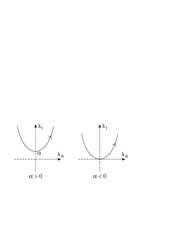
Figure 1: The contour $\partial D_{+}$ associated with Eq. (1a).

The long-time asymptotics

The representation obtained by the new method is convenient for computing the long-time asymptotics of the solution: Suppose that a given evolution PDE is valid for $0<t<T$, where $T$ is a positive constant. It can be shown (see section II) that the representation for $q(x,t)$ is equivalent to the representation obtained by replacing ${\hat{g}}(k,t)$ with ${\hat{g}}(k,T)$. In particular, if $0<t<\infty$, then ${\hat{g}}(k,t)$ can be replaced by ${\hat{g}}(k)\equiv{\hat{g}}(k,\infty)$. For example, the solution of the IBV (1) with $0<t<\infty$ is given by (11) with ${\hat{g}}(k,t)$ replaced by ${\hat{g}}(k)$,

$${\hat{g}}(k)=-{\hat{q}}_{0}(i\alpha-k)-(2ik+\alpha){\hat{g}}_{0}(k),\qquad{\hat{g}}_{0}(k)=\int_{0}^{\infty}dt\,e^{\omega(k)t}g_{0}(t).$$ (15)

Thus, the only time-dependence of $q(x,t)$ appears in the form $\exp[ikx-\omega(k)t]$; hence it is straightforward to obtain the long-time asymptotics, using the steepest descent method. Similar considerations are valid for evolution PDEs in multidimensions.

From the complex plane to the real axis

In case that the given IBV problem can be solved by an $x$-transform, the relevant representation can be obtained by deforming the integral representation of the solution obtained by the new method, from the complex $k$-plane to the real axis. Consider for example the integral in the r.h.s. of Eq. (11) for the case that $\alpha<0$: It can be verified that the functions $\exp(ikx)$, ${\hat{q}}_{0}(i\alpha-k)$, and $\exp[\omega(k)(\tau-t)]$ are bounded in the region of the complex $k$-plane above the real axis and below the curve $\partial D_{+}$. Thus, the integral along $\partial D_{+}$ can be deformed to an integral along the real axis,

$$q(x,t)=\frac{1}{2\pi}\int_{-\infty}^{\infty}dk\,e^{ikx-\omega(k)t}\left[{\hat{q}}_{0}(k)-{\hat{q}}_{0}(i\alpha-k)-(2ik+\alpha)\int_{0}^{t}d\tau\,e^{\omega(k)\tau}g_{0}(\tau)\right].$$ (16)

It can be shown that this formula is equivalent to the solution of Eqs. (9), (10) using the sine transform. However, if $\alpha>0$ this deformation is not possible. Indeed, ${\hat{q}}_{0}(i\alpha-k)$ involves $\exp[-ix(i\alpha-k)]=\exp[ik_{R}x]\exp[-x(k_{I}-\alpha)]$; this term is bounded for $k_{I}\geq\alpha$ (and in particular is bounded on $\partial D_{+}$), but it is not bounded in the region of the complex $k$-plane below the curve $\partial D_{+}$.

We note that even in the cases when it is possible to deform the contour to the real axis, the representation in the complex $k$-plane has certain advantages. For example, the integral involving the sine transform is not uniformly convergent at $x=0$ (unless $q(0,t)=0$). Also, a convenient way to study the long-time behavior of the representation involving the sine transform is to transform it to the associated representation in the complex $k$-plane.

II The Diffusion-Convection Equation

Physical significance

Eq. (1a) arises, for example, from the diffusion-convection equation

$$q_{\tau}=Dq_{\xi\xi}+\alpha vq_{\xi},\quad\alpha=\pm 1,\qquad 0<\xi<\infty,\quad\tau>0,$$ (17)

where $q(\xi,\tau)$ is a probability density function in the spatial and time variables $\xi$ and $\tau$, $D$ is a diffusion coefficient with dimensions of $({\rm length})^{2}/({\rm time})$, and $v$ is a convection field with dimensions of $({\rm length})/({\rm time})$. Eq. (1a) is the normalized form of (17), expressed in terms of the dimensionless variables $t=(D/v^{2})\tau$ and $x=(D/v)\xi$. The dependence upon the single spatial variable $x$ is justified in systems that are homogeneous in the transverse directions to $x$. The choice $\alpha=+1$ corresponds to convection (a background drift velocity $v$) directed toward the origin, while $\alpha=-1$ corresponds to a background drift away from the origin. In the long-time asymptotic limit convection dominates diffusion and determines the fate of the system. Suppose for example that the boundary condition is $q(0,t)=0$, corresponding to an ideal sink at the origin, for the case, of say, of particle flow. Then, if $\alpha=+1$ the particles will flow to the sink at typical speed $v$, and the probability density is expected to decay to zero exponentially with time. If $\alpha=-1$, the particles are drifting away from the sink; in this case one expects a depleted zone near the origin, which grows linearly with time, and exponential convergence to a finite level of survival. The case of generic boundary conditions is harder to predict by such heuristic arguments.

The method of images

We have seen that the method of images is applicable in the singular case of $\alpha=0$, and even then the solution is straightforward only with pure Dirichlet or von Neumann boundary conditions. For $\alpha<0$ the method of images can be used after a suitable transform, see Eqs. (10), and also provided that the boundary conditions are simple enough. For $\alpha>0$, the method of images fails to provide a solution for generic initial conditions. We now show how the new method serves as a natural extension of the methods of images and of classical integral transforms, even as these methods fail. For pedagogical reasons, we expose the new method simultaneously for problems (1) and (2). The physical interpretation of (2) is discussed in Section III.

The new method

Suppose that a linear evolution PDE in one space variable admits the solution $\exp[ikx-\omega(k)t]$. For well posedness we assume that

$${\rm Re}\,\omega(k)>0,\qquad{\rm for\ }k{\rm\ real}.$$ (18)

The starting point of the new method is to rewrite this PDE in the form

$$\left(e^{-ikx+\omega(k)t}q\right)_{t}+\left(e^{-ikx+\omega(k)t}X\right)_{x}=0,$$ (19)

where

$$X=-i\left(\frac{\omega(k)-\omega(l)}{k-l}\right)q,\qquad l=-i\partial_{x}.$$ (20)

For Eq. (1a), $\omega(k)=k^{2}-i\alpha k$, thus

$$X=-i\left(\frac{k^{2}-l^{2}-i\alpha(k-l)}{k-l}\right)q=-[i(k+l)+\alpha]q.$$

For Eq. (2a), $\omega(k)=i(k+k^{3})$, thus

$$X=\left(\frac{(k-l)+(k^{3}-l^{3})}{k-l}\right)q=(1+k^{2}+l^{2}+kl)q.$$

Hence Eqs. (1a) and (2a) can be written in the form (19), where $X$ is given, respectively, by

$$X=-q_{x}-(ik+\alpha)q,\qquad X=-q_{xx}-ikq_{x}+(1+k^{2})q.$$ (21)

(a) The Fourier transform representation

The solution of Eq. (19) can be expressed in the form

$$q(x,t)=\frac{1}{2\pi}\int_{-\infty}^{\infty}dk\,e^{ikx-\omega(k)t}{\hat{q}}_{0}(k)+\frac{1}{2\pi}\int_{-\infty}^{\infty}dk\,e^{ikx-\omega(k)t}{\hat{g}}(k,t),$$ (22)

where

$${\hat{q}}_{0}(k)=\int_{0}^{\infty}dx\,e^{-ikx}q_{0}(x),\qquad{\rm Im}\,k\leq 0,$$ (23)

$${\hat{g}}(k,t)=\int_{0}^{t}d\tau\,e^{\omega(k)\tau}X(0,\tau,k),\qquad k\in{\bf C}.$$ (24)

Furthermore, the functions ${\hat{q}}_{0}(k)$ and ${\hat{g}}(k,t)$ satisfy the global relation

$${\hat{g}}(k,t)+{\hat{q}}_{0}(k)=e^{\omega(k)t}{\hat{q}}(k,t),\qquad{\rm Im}\,k\leq 0,$$ (25)

where ${\hat{q}}(k,t)$ denotes the $x$-Fourier transform of $q(x,t)$.

Indeed, using (19) it is straightforward to compute the time evolution of ${\hat{q}}(k,t)$,

$$\left(e^{\omega(k)t}{\hat{q}}(k,t)\right)_{t} = \int_{0}^{\infty}dx\,\left(e^{-ikx+\omega(k)t}q(x,t)\right)_{t}$$

$$= -\int_{0}^{\infty}dx\,\left(e^{-ikx+\omega(k)t}X\right)_{x}=e^{\omega(k)t}X(0,t,k).$$

Integrating this equation we find Eq. (25). Solving Eq. (25) for ${\hat{q}}(k,t)$ and then using the inverse Fourier transform, we find Eq. (22).

(b) An integral representation in the complex k-plane

The first crucial step of the new method is to replace the second integral on the r.h.s. of Eq. (22) by an integral along the oriented curve $\partial D_{+}$. This curve is the boundary of the domain $D_{+}$,

$$D_{+}=\{k\in{\bf C},\>{\rm Im}\,k>0,\>{\rm Re}\,\omega(k)<0\},$$ (26)

oriented so that $D_{+}$ is on the left of $\partial D_{+}$. For example, for Eqs. (1a) and (2a) the domains $D_{+}$ are the shaded regions in Figs. 2 and 3, respectively. Each of the curves in Fig. 2 is defined by Eq. (12), while the curve in Fig. 3 is defined by

$$k_{I}=\sqrt{1+3k_{R}^{2}}.$$

Indeed, for Eq. (1a),

$${\rm Re}\,\omega(k)={\rm Re}\,\{(k_{R}+ik_{I})^{2}-i\alpha(k_{R}+ik_{I})\}=k_{R}^{2}-k_{I}^{2}+\alpha k_{I}.$$

Thus, $D_{+}$ is the domain of the upper half complex $k$-plane specified by

$$(k_{I}-\frac{\alpha}{2})^{2}-(k_{R}^{2}+(\frac{\alpha}{2})^{2})>0.$$

For Eq. (2a),

$${\rm Re}\,\omega(k)={\rm Re}\,\{i(k_{R}+ik_{I})^{3}+i(k_{R}+ik_{I})\}=k_{I}(k_{I}^{2}-3k_{R}^{2}-1).$$

Thus, $D_{+}$ is the domain of the upper half complex $k$-plane specified by

$$k_{I}^{2}-3k_{R}^{2}-1<0.$$

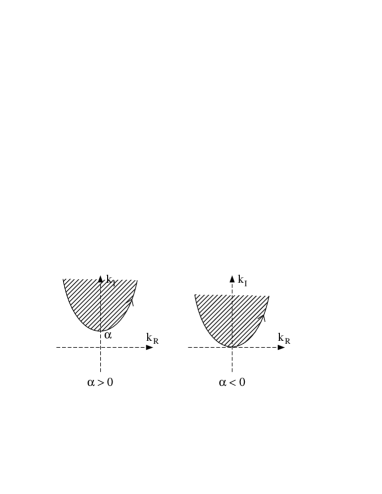
Figure 2: The domain $D_{+}$ for Eq. (1a).

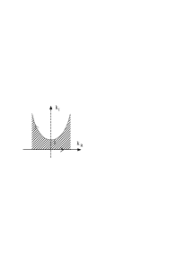
Figure 3: The domain $D_{+}$ for Eq. (2a).

The deformation of the integral from the real axis to the integral along the curve $\partial D_{+}$ is a direct consequence of Cauchy’s theorem. Indeed, the term

$$e^{ikx-\omega(k)t}{\hat{g}}(k,t)=e^{ikx}\int_{0}^{t}d\tau\,e^{-\omega(k)(t-\tau)}X(0,\tau,k)$$

is analytic and bounded in the domain $E_{+}$,

$$E_{+}=\{k\in{\bf C},\>{\rm Im}\,k>0,\>{\rm Re}\,\omega(k)>0\}.$$

Thus, using Jordan’s lemma in $E_{+}$, the integral along the boundary of $E_{+}$ vanishes.

For example, for Eq. (1a) $E_{+}$ is the domain above the real axis and below the curve $\partial D_{+}$; thus the integral along the real axis can be deformed to the integral along $\partial D_{+}$. For Eq. (2a), $E_{+}$ is the domain above the curve $\{k_{I}=\sqrt{1+3k_{R}^{2}}\}$, thus the integral along this curve vanishes; hence $\partial D_{+}$ is the union of the real axis and the curve $\{k_{I}=\sqrt{1+3k_{R}^{2}}\}$.

(c) Analysis of the global relation

The second crucial step in the new method is the analysis of the global relation (25): This yields ${\hat{g}}(k,t)$ in terms of ${\hat{q}}_{0}(k)$ and the $t$-transform of the given boundary conditions.

Before implementing this step, we note that we have already used Eq. (25) in the derivation of Eq. (22). However, while Eq. (25) was used earlier only for real $k$, in what follows it will be used in the complex $k$-plane.

Recall that ${\hat{g}}(k,t)$ is defined by Eq. (24), where for Eq. (1a) $X$ is given by (21a). Thus

$${\hat{g}}(k,t)=-{\hat{g}}_{1}(\omega(k),t)-(ik+\alpha){\hat{g}}_{0}(\omega(k),t),\qquad\omega(k)=k^{2}-i\alpha k,$$ (27)

where

$${\hat{g}}_{1}(\omega(k),t)=\int_{0}^{t}d\tau\,e^{\omega(k)\tau}q_{x}(0,\tau),\quad{\hat{g}}_{0}(\omega(k),t)=\int_{0}^{t}d\tau\,e^{\omega(k)\tau}g_{0}(\tau);$$

we have used the notation ${\hat{g}}_{1}(\omega(k),t)$ and ${\hat{g}}_{0}(\omega(k),t)$ to emphasize that ${\hat{g}}_{1}$ and ${\hat{g}}_{0}$ depend on $k$ only through $\omega(k)$. Substituting the expression for ${\hat{g}}(k,t)$ from (27) into the global relation (25) we find

$$-{\hat{g}}_{1}(\omega(k),t)=(ik+\alpha){\hat{g}}_{0}(\omega(k),t)-{\hat{q}}_{0}(k)+e^{\omega(k)t}{\hat{q}}(k,t),\qquad{\rm Im}\,k\leq 0.$$ (28)

Our task is to compute ${\hat{g}}(k,t)$ on the curve $\partial D_{+}$; since ${\hat{g}}(k,t)$ is analytic in $D_{+}$ this is equivalent to computing ${\hat{g}}(k,t)$ for $k\in D_{+}$. Eq. (27) shows that ${\hat{g}}(k,t)$ involves ${\hat{g}}_{0}$, which is known in terms of the given boundary condition $g_{0}(t)$, as well as ${\hat{g}}_{1}$, which involves the unknown boundary value $q_{x}(0,t)$. In order to compute ${\hat{g}}_{1}$ using the global relation (28), we first transform Eq. (28) from the lower half complex $k$-plane to the domain $D_{+}$. In this respect, it is important to observe that since ${\hat{g}}_{1}$ depends on $k$ only through $\omega(k)$, ${\hat{g}}_{1}$ remains invariant by those transformations $k\to\nu(k)$ which preserve $\omega(k)$. For Eq. (1a), the equation $\omega(k)=\omega(\nu(k))$ has one non-trivial root (the trivial root is $\nu(k)=k$),

$$\nu^{2}-i\alpha\nu=k^{2}-i\alpha k,\qquad\nu(k)=i\alpha-k.$$

Let $D_{-}$ be defined by

$$D_{-}=\{k\in{\bf C},\>{\rm Im}\,k<0,\>{\rm Re}\,\omega(k)<0\}.$$ (29)

For $\omega(k)=k^{2}-i\alpha k$, the domains $D_{+}$ and $D_{-}$ are the shaded regions depicted in Fig. 4. The transformations that leave $\omega(k)$ invariant map the domain $\{D_{+}\oplus D_{-}\}$ onto itself. Thus, if $k\in D_{+}$, then $i\alpha-k\in D_{-}$. Hence, replacing $k$ by $i\alpha-k$ in Eq. (28), we find an equation that is valid for $k$ in $D_{+}$:

$$-{\hat{g}}_{1}=-ik{\hat{g}}_{0}-{\hat{q}}_{0}(i\alpha-k)+e^{\omega(k)t}{\hat{q}}(i\alpha-k,t),\qquad k\in D_{+}.$$ (30)

Replacing $-{\hat{g}}_{1}$ in (27) by the r.h.s. of the above equation, we find

$${\hat{g}}(k,t)=-(2ik+\alpha){\hat{g}}_{0}(\omega(k),t)-{\hat{q}}_{0}(i\alpha-k)+e^{\omega(k)t}{\hat{q}}(i\alpha-k,t).$$

The term $e^{\omega(k)t}{\hat{q}}(i\alpha-k,t)$ does not contribute to $q(x,t)$. Indeed, this term gives rise to the integral

$$\int_{\partial D_{+}}dk\,e^{ikx}{\hat{q}}(i\alpha-k,t),$$

for which we note: $\exp(ikx)$ is bounded and analytic for ${\rm Im}\,k>0$; the term ${\hat{q}}(i\alpha-k,t)$ involves $\exp[-i(i\alpha-k)x]=\exp(ik_{R}x)\exp[-x(k_{I}-\alpha)]$, which is bounded and analytic for $k_{I}>\alpha$, i.e., in $D_{+}$. Thus using Jordan’s lemma in $D_{+}$ it follows that the above integral vanishes, hence the effective part of ${\hat{g}}(k,t)$ is given by (14).

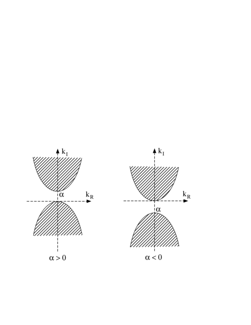
Figure 4: The domains $D_{+}$ and $D_{-}$ associated with Eq. (1a).

(d) The long-time asymptotics

Suppose that a given evolution PDE is valid for $0<t<T$, where $T$ is a positive constant. Then, as mentioned earlier, we can replace ${\hat{g}}(k,t)$ by ${\hat{g}}(k,T)$. Indeed, the two representations associated with ${\hat{g}}(k,t)$ and ${\hat{g}}(k,T)$ differ by

$$\int_{\partial D_{+}}dk\,e^{ikx-\omega(k)t}\int_{t}^{T}d\tau\,e^{\omega(k)\tau}X(0,\tau,k).$$

Since $T\geq t$, the coefficient $(\tau-t)$ of $\omega(k)$ is non-negative, thus $\exp[ikx+\omega(k)(\tau-t)]$ is bounded and analytic in $D_{+}$, and Jordan’s lemma implies that the above integral vanishes.

In the case of Eq. (1a) the solution is given by Eqs. (11)-(13), Eq. (15). The long-time asymptotics of $q(x,t)$ can be analyzed by the method of steepest descent. For $x=vt$, the critical point occurs at $d\omega/dk=iv$, or

$$k=\frac{i}{2}(\alpha+v)\equiv i\gamma.$$

Let $v>\alpha>0$, then both integrals on the r.h.s. of (11) contribute to the long-time asymptotics, since the path of integration can be modified to pass through the critical point in each case. The behaviour of the argument of the relevant exponentials near the critical point is given by

$$ikvt-\omega(k)t=-\gamma^{2}t-(k-i\gamma)^{2}t,$$

hence the leading-order asymptotics to $q(vt,t)$ is

$$\frac{1}{2\pi}{\hat{q}}_{0}(i\gamma)e^{-\gamma^{2}t}\int_{-\infty}^{\infty}e^{-(k-i\gamma)^{2}t}dk+\frac{1}{2\pi}{\hat{g}}(i\gamma)e^{-\gamma^{2}t}\int_{\partial D_{+}}e^{-(k-i\gamma)^{2}t}dk=\frac{1}{2\sqrt{\pi t}}[{\hat{q}}_{0}(i\gamma)+{\hat{g}}(i\gamma)]e^{-\gamma^{2}t}.$$

The numerical value of ${\hat{q}}_{0}(i\gamma)$ and ${\hat{g}}(i\gamma)$ are given explicitly in terms of the initial and boundary conditions, see Eqs. (13) and (15).

For $\alpha>v>0$ the second integral on the r.h.s. of (11) does not contribute, since the critical point lies outside of the domain $D_{+}$. In this case the leading-order asymptotics is

$$q(vt,t)\sim\frac{1}{2\sqrt{\pi t}}{\hat{q}}_{0}(i\gamma)e^{-\gamma^{2}t}.$$

For $\alpha<0$ and $v>-\alpha$ both integrals contribute and the answer is identical with that of the case $v>\alpha>0$. Finally, for $\alpha<0$ and $v<-\alpha$ neither integral contributes and the leading-order asymptotic behavior is zero. The latter is expected on physical grounds, since the (rightward) drift sweeps the probability density $q(vt,t)$ past $x=vt$.

III The Linearized Korteweg - de Vries Equation

Eq. (2a) is the linear limit of the celebrated Korteweg - de Vries equation:

$$q_{t}+q_{x}+\lambda q_{xxx}+6qq_{x}=0,\quad\lambda=\pm 1,$$ (31)

for the case of $\lambda=-1$; this corresponds to dominant surface tension. Eq. (31) is the normalized form of

$$\frac{\partial\eta}{\partial\tau}=\frac{3}{2}\sqrt{\frac{g}{h}}\frac{\partial}{\partial\xi}(\frac{1}{2}\eta^{2}+\eta+\frac{1}{3}\sigma\frac{\partial^{2}\eta}{\partial\xi^{2}}),\qquad\sigma=\frac{1}{8}h^{3}-\frac{Th}{\rho g},$$ (32)

where $\eta$ is the elevation of the water above the equilibrium level $h$, $T$ is the surface tension, $\rho$ is the density of the medium, and $g$ is the free-fall acceleration constant. This equation is the small amplitude, long wave limit of the equations describing idealized (inviscid) water waves under the assumption of irrotationality. Eq. (31) is obtained after transforming to the dimensionless variables $t=\frac{1}{2}\sqrt{\frac{g}{h\sigma}}\tau$, $x=-\sigma^{-1/2}\xi$, $q=\eta/2$.

Eq. (31) usually appears without the $q_{x}$ term. This is because the Korteweg - de Vries equation is usually studied on the full line and then the term $q_{x}$ can be eliminated by means of a Galilean transformation. However, for the half-line this transformation would change the domain from a quarter-plane to a wedge.

Laboratory experiments with water waves typically involve Eq. (31) with $\lambda=1$, $q(x,0)=0$, and $q(0,t)$ a periodic function of $t$. Thus the linearized version of Eq. (31) with $\lambda=1$ is valid until small amplitude waves reach the opposite end of the water tank. Eq. (2a) is valid under similar circumstances, in the case of dominant surface tension.

It is interesting to note that while in the case of $\lambda=1$ the problem is well posed with only one boundary condition at $x=0$, in the case of $\lambda=-1$ the problem is well posed with two boundary conditions. The case of $\lambda=1$ is solved in IMA . Here we solve the case of $\lambda=-1$.

The solution of the IBV problem (2) is given by Eq. (11), where $\omega(k)=i(k+k^{3})$, ${\hat{q}}_{0}(k)$ is the Fourier transform of $q_{0}(x)$ (see Eq. (13)), ${\hat{g}}(k,t)$ is defined by

$${\hat{g}}(k,t)=-{\hat{q}}_{0}(\nu)+i(\nu-k)\int_{0}^{t}d\tau\,e^{\omega(k)\tau}g_{1}(\tau)+(k^{2}-\nu^{2})\int_{0}^{t}d\tau\,e^{\omega(k)\tau}g_{0}(\tau),$$ (33)

$$\nu=\frac{-k-i\sqrt{3k^{2}+4}}{2}\>\>{\rm for\ }k\in D_{+}^{(1)},\qquad\nu=\frac{-k+i\sqrt{3k^{2}+4}}{2}\>\>{\rm for\ }k\in D_{+}^{(2)},$$

and $\partial D_{+}$ is the union of the boundaries of $D_{+}^{(1)}$ and $D_{+}^{(2)}$ depicted in Fig. 5 (the relevant curve is $\{k_{I}=\sqrt{3k_{R}^{2}+1},\,k_{I}>0\}$).

Indeed, the representation (11) was derived in section II. Using the definition of ${\hat{g}}(k,t)$, Eq. (24), and recalling that $X$ is given by Eq. (21b), we find

$${\hat{g}}(k,t)=-{\hat{g}}_{2}(\omega(k),t)-ik{\hat{g}}_{1}(\omega(k),t)+(1+k^{2}){\hat{g}}_{0}(\omega(k),t),\qquad\omega(k)=i(k+k^{3}),$$ (34)

where ${\hat{g}}_{1}$, ${\hat{g}}_{0}$ are the first, second integrals appearing in the r.h.s. of Eq. (33) and ${\hat{g}}_{2}$ involves the unknown boundary value $q_{xx}(0,t)$,

$${\hat{g}}_{2}(\omega(k),t)=\int_{0}^{t}d\tau\,e^{\omega(k)\tau}q_{xx}(0,\tau).$$

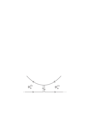
Figure 5: The contours $\partial D_{+}^{(1)}$ and $\partial D_{+}^{(2)}$ associated with Eq. (2a).

Substituting the expression for ${\hat{g}}(k,t)$ from Eq. (34) into the global relation (25), we find

$$-{\hat{g}}_{2}(\omega(k),t)=ik{\hat{g}}_{1}(\omega(k),t)-(1+k^{2}){\hat{g}}_{0}(\omega(k),t)-{\hat{q}}_{0}(k)+e^{\omega(k)t}{\hat{q}}(k,t),\qquad{\rm Im}\,k\leq 0.$$ (35)

The equation $\omega(k)=\omega(\nu(k))$ has two nontrivial roots,

$$\nu+\nu^{3}=k+k^{3},\qquad\nu^{2}+k\nu+k^{2}+1=0,\qquad\nu_{1,2}=\frac{-k\mp i\sqrt{3k^{2}+4}}{2};$$ (36)

$$\nu_{1}(k)\sim e^{4i\pi/3}k,\qquad\nu_{2}(k)\sim e^{2i\pi/3}k,\qquad k\to\infty.$$

The domains $D_{+}$ and $D_{-}$ (see Eqs. (26) and (29)) are the shaded regions depicted in Fig. 6a, where the two relevant curves are $k_{I}=\pm\sqrt{3k_{R}^{2}+1}$; the limit of the domains as $k\to\infty$ are depicted in Fig. 6b, where each of the relevant angles is $\pi/3$.

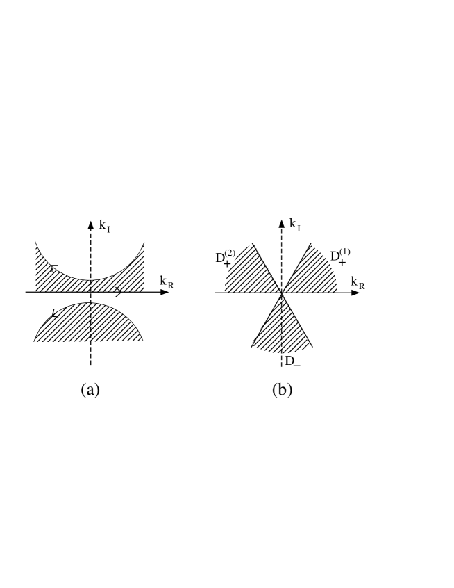
Figure 6: The domains $D_{+}$ and $D_{-}$ for Eq. (2a).

If $\frac{2\pi}{3}<\arg k<\frac{4\pi}{3}$ then $\frac{4\pi}{3}<\arg k+\frac{2\pi}{3}<2\pi$, and $2\pi<\arg k+\frac{4\pi}{3}<\frac{8\pi}{3}$. Thus

$$k\in D_{+}^{(2)},\qquad\nu_{2}(k)\in D_{-},\qquad\nu_{1}(k)\in D_{+}^{(1)}.$$

Similarly,

$$k\in D_{+}^{(1)},\qquad\nu_{2}(k)\in D_{+}^{(2)},\qquad\nu_{1}(k)\in D_{-}.$$

Thus, replacing $k$ by $\nu_{1}(k)$ and $\nu_{2}(k)$ in (35), we find

$$-{\hat{g}}_{2}=i\nu_{1}{\hat{g}}_{1}-(1+\nu_{1}^{2}){\hat{g}}_{0}-{\hat{q}}_{0}(\nu_{1})+e^{\omega(k)t}{\hat{q}}(\nu_{1}(k),t),\qquad k\in D_{+}^{(1)};$$

$$-{\hat{g}}_{2}=i\nu_{2}{\hat{g}}_{1}-(1+\nu_{2}^{2}){\hat{g}}_{0}-{\hat{q}}_{0}(\nu_{2})+e^{\omega(k)t}{\hat{q}}(\nu_{2}(k),t),\qquad k\in D_{+}^{(2)}.$$

Replacing $-{\hat{g}}_{2}$ in (34) by the r.h.s. of the above equations, we find

$${\hat{g}}(k,t)=i(\nu-k){\hat{g}}_{1}+(k^{2}-\nu^{2}){\hat{g}}_{0}-{\hat{q}}_{0}(\nu)+e^{\omega(k)t}{\hat{q}}(\nu,t),\qquad k\in D_{+}.$$

Due to analiticity considerations the term ${\hat{q}}(\nu,t)$ does not contribute to $q(x,t)$, see section II; thus the effective part of ${\hat{g}}(k,t)$ is given by (33).

The long-time asymptotics

The long-time asymptotics can again be analyzed by replacing ${\hat{g}}(k,t)$ with ${\hat{g}}(k,\infty)={\hat{g}}(k)$ and following standard steepest descent or stationary phase expansions. One thus finds F-Schultz : For $v=x/t>1$, $q(vt,t)$ satisfies

$$q(vt,t)=\frac{1}{\sqrt{12\pi\gamma t}}\big{[}(P(\gamma)-P(\nu(\gamma))e^{i\varphi}+(P(-\gamma)-P(\nu(-\gamma))e^{-i\varphi}\big{]}+{\cal O}(t^{-3/2}),$$

as $t\to\infty$, where

$$\gamma = \sqrt{\frac{v-1}{3}},$$

$$\varphi(t) = 2\gamma^{3}t-\pi/4,$$

$$\nu(k) = -\frac{1}{2}(k+i\sqrt{3k^{2}+4}),$$

$$P(k) = {\hat{q}}_{0}(k)+(k^{2}+1){\hat{g}}_{0}(k)-ik{\hat{g}}_{1}(k),$$

${\hat{q}}_{0}(k)$ is defined in terms of the initial condition (Eq. (15)), and ${\hat{g}}_{1}(k)$, ${\hat{g}}_{0}(k)$ are the first, second integrals appearing in the r.h.s. of Eq. (33) evaluated with $t\to\infty$. For $v<1$, $q(vt,t)$ decays faster than any algebraic power of $t$, as $t\to\infty$.

IV The Diffusion Equation in Multidimensions

Physical significance

This problem is the generalization of problem (1) to multidimensions. It arises from the diffusion-convection equation

$$q_{\tau}=\sum_{j=1}^{N}(Dq_{\xi_{j}\xi_{j}}+v_{j}q_{\xi_{j}}),\qquad 0<\xi_{j}<\infty,\quad\tau>0,\quad j=1,2,\dots N,$$ (37)

which represent isotropic diffusion in a quadrant of $N$-dimensional space, with diffusion coefficient $D$, and under a background convection (drift) field $(v_{1},v_{2},\dots,v_{N})$. Eq. (3a) is obtained upon passing to the dimensionless variables $t=(D/{\bar{v}}^{2})\tau$ and $x_{j}=(D/{\bar{v}})\xi_{j}$, $j=1,2,\dots,N$, where ${\bar{v}}$ is a typical speed such as the rms ${\bar{v}}=(\sum_{j}v_{j}^{2})^{1/2}$.

The new method

For the solution of the IBV problem (3) we introduce the following notations:

$$\bullet\quad x=(x_{1},\dots,x_{N}),\qquad k=(k_{1},\dots,k_{N}),\qquad k\cdot x=\sum_{1}^{N}k_{l}x_{l},\qquad k^{(j)}\cdot x^{(j)}=\sum_{l=1,l\neq j}^{N}k_{l}x_{l}.$$

$$\bullet\quad\int_{{\bf R}^{N}}dk=\int_{-\infty}^{\infty}dk_{1}\cdots\int_{-\infty}^{\infty}dk_{N}.$$

$$\bullet\quad C_{j}\text{\ is the curve\ }\{(k_{j})_{I}>0,\>(k_{j})_{I}=\frac{\alpha_{j}}{2}+\sqrt{[(k_{j})_{R}]^{2}+(\frac{\alpha_{j}}{2})^{2}},\>j=1,2,\dots,N\}.$$

$$\bullet\quad\nu_{j}=i\alpha_{j}-k_{j},\qquad j=1,2,\dots,N.$$

$$\bullet\quad\omega(k)=\sum_{j=1}^{N}(k_{j}^{2}-i\alpha_{j}k_{j}).$$

$$\bullet\quad{\hat{q}}_{0}(k)=\int_{0}^{\infty}dx_{1}\cdots\int_{0}^{\infty}dx_{N}\,e^{-ik\cdot x}q_{0}(x).$$

$$\bullet\quad{\hat{g}}_{0}^{(j)}(k,t)=\int_{0}^{t}d\tau\int_{0}^{\infty}dx_{1}\cdots\int_{0}^{\infty}dx_{j-1}\int_{0}^{\infty}dx_{j+1}\cdots\int_{0}^{\infty}dx_{N}\,e^{-ik^{(j)}\cdot x^{(j)}+\omega(k)\tau}g_{0}^{(j)}(x_{1},\dots,x_{j-1},x_{j+1},\dots,x_{N},\tau),$$

$$\quad\>\>j=1,2,\dots,N.$$

$$\bullet\quad{\hat{Q}}(k,t)={\hat{q}}_{0}(k)-\sum_{1}^{N}(ik_{j}+\alpha_{j}){\hat{g}}_{0}^{(j)}(k,t).$$

The solution of the IBV problem (3) is given by

$$q(x,t)= \frac{1}{(2\pi)^{N}}\int_{{\bf R}^{N}}dk\,e^{ik\cdot x-\omega(k)t}{\hat{q}}_{0}(k)$$ (38)

$$-\frac{1}{(2\pi)^{N}}\sum_{1}^{N}\int_{-\infty}^{\infty}dk_{1}\cdots\int_{-\infty}^{\infty}dk_{j-1}\int_{C_{j}}dk_{j}\int_{-\infty}^{\infty}dk_{j+1}\cdots\int_{-\infty}^{\infty}dk_{N}\,e^{ik\cdot x-\omega(k)t}(ik_{j}+\alpha_{j}){\hat{g}}_{0}^{(j)}(k,t)$$

$$-\frac{1}{(2\pi)^{N}}\left(\int_{C_{1}}dk_{1}\int_{-\infty}^{\infty}dk_{2}\cdots\int_{-\infty}^{\infty}dk_{N}e^{ik\cdot x-\omega(k)t}{\hat{Q}}(\nu_{1},k_{2},\dots,k_{N})+CP\right)$$

$$+\frac{1}{(2\pi)^{N}}\left(\int_{C_{1}}dk_{1}\int_{C_{2}}dk_{2}\int_{-\infty}^{\infty}dk_{3}\cdots\int_{-\infty}^{\infty}dk_{N}e^{ik\cdot x-\omega(k)t}{\hat{Q}}(\nu_{1},\nu_{2},k_{3},\dots,k_{N})+CP\right)$$

$$-\cdots+\frac{(-1)^{N}}{(2\pi)^{N}}\int_{C_{1}}dk_{1}\int_{C_{2}}dk_{2}\cdots\int_{C_{N}}dk_{N}\,e^{ik\cdot x-\omega(k)t}{\hat{Q}}(\nu_{1},\nu_{2},\dots,\nu_{N}),$$

where $CP$ denotes cyclic permutations (i.e., all possible relevant combinations).

For the derivation of Eq. (38) we introduce the additional notations:

$$\bullet\quad x^{(j)}=(x_{1},\dots,x_{j-1},x_{j+1},\dots,x_{N}),\qquad k^{(j)}=(k_{1},\dots,k_{j-1},k_{j+1},\dots,k_{N}).$$

$$\bullet\quad\int_{{\bf R}_{+}^{N}}dx=\int_{0}^{\infty}dx_{1}\cdots\int_{0}^{\infty}dx_{N}.$$

$$\bullet\quad\int_{{\bf R}_{+}^{(j)}}dx^{(j)}=\int_{0}^{\infty}dx_{1}\cdots\int_{0}^{\infty}dx_{j-1}\int_{0}^{\infty}dx_{j+1}\cdots\int_{0}^{\infty}dx_{N}.$$

$$\bullet\quad\int_{{\bf R}^{(j)}}dk^{(j)}=\int_{-\infty}^{\infty}dk_{1}\cdots\int_{-\infty}^{\infty}dk_{j-1}\int_{-\infty}^{\infty}dk_{j+1}\cdots\int_{-\infty}^{\infty}dk_{N}.$$

$$\bullet\quad e=e^{ik\cdot x-\omega(k)t}.$$

$$\bullet\quad E=e^{\omega(k)t}.$$

Substituting $\exp[ik\cdot x-\omega(k)t]$ in Eq. (3a) we find that $\omega(k)$ is given by the expression defined in the notations.

Eq. (3a) can be written in the form

$$\left(e^{-ik\cdot x+\omega(k)t}q\right)_{t}+\sum_{1}^{N}\left(e^{-ik\cdot x+\omega(k)t}X_{j}\right)_{x_{j}}=0,$$ (39)

where

$$X_{j}=-q_{x_{j}}-(ik_{j}+\alpha_{j})q,\qquad j=1,2,\dots,N.$$

Let ${\hat{q}}(k,t)$ denote the $N$-dimensional Fourier transform of $q(x,t)$. Using Eq. (39) we find

$$\left(e^{\omega(k)t}{\hat{q}}(k,t)\right)_{t} =\int_{{\bf R}_{+}^{N}}dx\,\Big{(}e^{-ik\cdot x+\omega(k)t}q(x,t)\Big{)}_{t}$$

$$=-\sum_{j=1}^{N}\int_{0}^{\infty}dx_{j}\Big{(}e^{-ik\cdot x+\omega(k)t}X_{j}\Big{)}_{x_{j}}=\sum_{j=1}^{N}e^{-ik\cdot x+\omega(k)t}X_{j}|_{x_{j}=0}.$$

Integrating this equation with respect to $t$, we obtain

$${\hat{q}}_{0}(k)+\sum_{1}^{N}{\hat{g}}^{(j)}(k,t)=e^{\omega(k)t}{\hat{q}}(k,t),$$ (40)

where ${\hat{q}}_{0}(k)$ is the $N$-dimensional Fourier transform of $q_{0}(x)$ and ${\hat{g}}^{(j)}(k,t)$ is defined as follows:

$${\hat{g}}^{(j)}(k,t)=-\int_{0}^{t}d\tau\int_{{\bf R}_{+}^{(j)}}dx^{(j)}\,e^{-ik^{(j)}\cdot x^{(j)}+\omega(k)\tau}[q_{x_{j}}(x^{(j)},\tau)+(ik_{j}+\alpha_{j})q(x^{(j)},\tau)],$$

or

$${\hat{g}}^{(j)}(k,t)\equiv{\hat{g}}_{1}^{(j)}(-ik^{(j)},\omega(k),t)-(ik_{j}+\alpha_{j}){\hat{g}}_{0}^{(j)}(-ik^{(j)},\omega(k),t),\qquad j=1,2,\dots,N,$$ (41)

where ${\hat{g}}_{0}^{(j)}$ is defined in the notations and ${\hat{g}}_{1}^{(j)}$ denotes the integral of $-q_{x_{j}}$.

Solving Eq. (40) for ${\hat{q}}(k,t)$ and using the inverse $N$-dimensional Fourier transform, we find

$$q(x,t)=\frac{1}{(2\pi)^{N}}\int_{{\bf R}^{N}}dk\,e^{ik\cdot x-\omega(k)t}{\hat{q}}_{0}(k)+\frac{1}{(2\pi)^{N}}\sum_{1}^{N}\int_{{\bf R}^{N}}dk\,e^{ik\cdot x-\omega(k)t}[{\hat{g}}_{1}^{(j)}-(ik_{j}+\alpha_{j}){\hat{g}}_{0}^{(j)}].$$ (42)

The terms ${\hat{g}}_{1}^{(j)}$ and ${\hat{g}}_{0}^{(j)}$ contain $k_{j}$ only through $\omega(k)$, thus the relevant integral in the complex $k_{j}$-plane can be deformed from the real axis to the curve $C_{j}$ (see the discussion in section II). Hence Eq. (42) yields the first two integrals appearing in (38) plus the term

$$\frac{1}{(2\pi)^{N}}\sum_{1}^{N}\int_{{\bf R}^{(j)}}dk^{(j)}\int_{C_{j}}dk_{j}\,e^{ik\cdot x-\omega(k)t}{\hat{g}}_{1}^{(j)}.$$ (43)

Using the global relation (40), it can be shown that the above term yields the remaining expressions appearing in (38). For pedagogical reasons, we give the details for $N=3$: In this case the global condition becomes

$${\hat{g}}_{1}^{(1)}(-ik_{2},-ik_{3})+{\hat{g}}_{1}^{(2)}(-ik_{1},-ik_{3})+{\hat{g}}_{1}^{(3)}(-ik_{2},-ik_{3})=-{\hat{Q}}(k_{1},k_{2},k_{3})+E{\hat{q}}(k_{1},k_{2},k_{3}),\qquad{\rm Im}\,k_{j}\leq 0,$$ (44)

where $E$, ${\hat{Q}}$ are defined in the notations and, for simplicity of notation, we have dropped the $t$- and $\omega(k)$-dependence. Since ${\hat{g}}_{1}^{(1)}$ in Eq. (43) is integrated along $C_{1}$, we replace $k_{1}$ by $\nu_{1}$ in Eq. (44) and then solve the resulting equation for ${\hat{g}}_{1}^{(1)}(-ik_{2},-ik_{3})$. Similarly, for ${\hat{g}}_{1}^{(2)}$, ${\hat{g}}_{1}^{(3)}$, we replace $k_{2}$, $k_{3}$ in Eq. (44) by $\nu_{2}$, $\nu_{3}$. Thus the expression (43) becomes

$$-\int_{{\bf R}^{2}}dk_{2}dk_{3}\int_{C_{1}}dk_{1}\,e[{\hat{g}}_{1}^{(2)}(-i\nu_{1},-ik_{3})+{\hat{g}}_{1}^{(3)}(-i\nu_{1},-ik_{2})]$$

$$-\int_{{\bf R}^{2}}dk_{1}dk_{3}\int_{C_{2}}dk_{2}\,e[{\hat{g}}_{1}^{(1)}(-i\nu_{2},-ik_{3})+{\hat{g}}_{1}^{(3)}(-ik_{1},-i\nu_{2})]$$

$$-\int_{{\bf R}^{2}}dk_{1}dk_{2}\int_{C_{3}}dk_{3}\,e[{\hat{g}}_{1}^{(1)}(-ik_{2},-i\nu_{3})+{\hat{g}}_{1}^{(2)}(-ik_{1},-i\nu_{3})]$$ (45)

$$-\int_{{\bf R}^{2}}dk_{2}dk_{3}\int_{C_{1}}dk_{1}\,e{\hat{Q}}(\nu_{1},k_{2},k_{3})-\int_{{\bf R}^{2}}dk_{1}dk_{3}\int_{C_{2}}dk_{2}\,e{\hat{Q}}(k_{1},\nu_{2},k_{3})-\int_{{\bf R}^{2}}dk_{1}dk_{2}\int_{C_{3}}dk_{3}\,e{\hat{Q}}(k_{1},k_{2},\nu_{3}).$$

In addition to these terms we obtain three terms involving ${\hat{q}}$, but these terms vanish due to analyticity considerations; for example, one of these terms is

$$\int_{{\bf R}^{2}}dk_{2}dk_{3}\int_{C_{1}}dk_{1}\,e^{ik\cdot x}{\hat{q}}(\nu_{1},k_{2},k_{3},t),$$

which vanishes since both $e^{ik\cdot x}$ and ${\hat{q}}(\nu_{1},k_{2},k_{3},t)$ are bounded and analytic in the region of the complex $k_{1}$-plane above the curve $C_{1}$.

The last 3 terms in  (IV) are part of the expression for $q(x,t)$; regarding the first 3 terms in (IV), we note the following: the two integrals involving ${\hat{g}}^{(2)}$ contain $k_{2}$ only through $\omega(k)$, thus for these integrals the contour with respect to $k_{2}$ can be deformed from the real $k_{2}$-axis to the curve $C_{2}$; similarly for the integrals involving ${\hat{g}}^{(1)}$ and ${\hat{g}}^{(3)}$. Thus we obtain

$$-\int_{{\bf R}}dk_{3}\int_{C_{2}}dk_{2}\int_{C_{1}}dk_{1}\,e[{\hat{g}}_{1}^{(1)}(-i\nu_{2},-ik_{3})+{\hat{g}}_{1}^{(2)}(-i\nu_{1},-ik_{3})],$$ (46)

plus two more similar integrals, which can be obtained from (46) by cyclic permutation $1\to 2\to 3\to 1$. The square bracket appearing in (46) can be expressed in terms of ${\hat{g}}_{1}^{(3)}$ using the global relation evaluated at $k_{1}\to\nu_{1}$, $k_{2}\to\nu_{2}$,

$$-{\hat{g}}_{1}^{(1)}(-i\nu_{2},-ik_{3})-{\hat{g}}_{1}^{(2)}(-i\nu_{1},-ik_{3})={\hat{g}}_{1}^{(3)}(-i\nu_{1},-i\nu_{2})+{\hat{Q}}(\nu_{1},\nu_{2},k_{3})-E{\hat{q}}(\nu_{1},\nu_{2},k_{3}).$$

Due to analyticity considerations the term involving ${\hat{q}}$ vanishes, thus the expression (46) together with the other two similar expressions yield

$$\int_{\bf R}dk_{3}\int_{C_{2}}dk_{2}\int_{C_{1}}dk_{1}\,e{\hat{g}}_{1}^{(3)}(-i\nu_{1},-i\nu_{2})+\int_{\bf R}dk_{2}\int_{C_{3}}dk_{3}\int_{C_{1}}dk_{1}\,e{\hat{g}}_{1}^{(2)}(-i\nu_{1},-i\nu_{3})$$

$$+\int_{\bf R}dk_{1}\int_{C_{2}}dk_{2}\int_{C_{3}}dk_{3}\,e{\hat{g}}_{1}^{(1)}(-i\nu_{2},-i\nu_{3})$$

$$+\int_{\bf R}dk_{3}\int_{C_{2}}dk_{2}\int_{C_{1}}dk_{1}\,e{\hat{Q}}(\nu_{1},\nu_{2},k_{3})+\int_{\bf R}dk_{2}\int_{C_{3}}dk_{3}\int_{C_{1}}dk_{1}\,e{\hat{Q}}(\nu_{1},k_{2},\nu_{3})$$

$$+\int_{\bf R}dk_{1}\int_{C_{2}}dk_{2}\int_{C_{3}}dk_{3}\,e{\hat{Q}}(k_{1},\nu_{2},\nu_{3}).$$ (47)

The last three terms above, are part of the expression for $q(x,t)$; regarding the first three terms we note the following: the integral involving ${\hat{g}}^{(3)}$ contains $k_{3}$ only through $\omega(k)$, thus the integration along the real $k_{3}$-axis can be deformed to the curve $C_{3}$; similarly for the other two integrals. Thus the first three terms of (IV) yield

$$\int_{C_{1}}dk_{1}\int_{C_{2}}dk_{2}\int_{C_{3}}dk_{3}\,e[{\hat{g}}_{1}^{(1)}(-i\nu_{2},-i\nu_{3})+{\hat{g}}_{1}^{(2)}(-i\nu_{1},-i\nu_{3})+{\hat{g}}_{1}^{(3)}(-i\nu_{1},-i\nu_{2})].$$ (48)

Using the global relation evaluated at $k_{1}\to\nu_{1}$, $k_{2}\to\nu_{2}$, $k_{3}\to\nu_{3}$, the square bracket appearing in (48) can be replaced by

$$-{\hat{Q}}(\nu_{1},\nu_{2},\nu_{3})+E{\hat{q}}(\nu_{1},\nu_{2},\nu_{3},t).$$

Thus the expression (48) yields

$$-\int_{C_{1}}dk_{1}\int_{C_{2}}dk_{2}\int_{C_{3}}dk_{3}\,e{\hat{Q}}(\nu_{1},\nu_{2},\nu_{3})$$

plus a term involving ${\hat{q}}$ that vanishes due to analiticity considerations.

The long-time asymptotics

The long-time asymptotics may be analyzed by the method of steepest descent, after replacing the variables ${\hat{g}}^{(j)}(k,t)$ with ${\hat{g}}^{(j)}(k)={\hat{g}}^{(j)}(k,\infty)$.

References

(1) A. S. Fokas “A unified transform Method for linear and
certain nonlinear PDEs”, Proc. R. Soc. 53, 1411 (1997).
(2) A. S. Fokas, “A new transform method for evolution PDEs,” IMA
J. Appl. Math. 67, 559 (2002).
(3) A. S. Fokas and B. Pelloni, “Two point boundary
value problems for linear evolution equations”, Math. Proc. Camb.
Phil. Soc. 131, 521 (2001).
(4) B. Pelloni, Math. Proc. Camb. Phil. Soc. (in press).
(5) A. S. Fokas, “Two dimensional linear PDEs in a
convex polygon”, Proc. R. Soc. 457 371 (2001).
(6) A. S. Fokas and A. A. Kapaev, “On a transform
method for the Laplace equation in a polygon”, IMA J. Appl. Math.
68 (2003).
(7) D. ben-Avraham and A. S. Fokas, “The solution of the modified
Helmholtz equation in a wedge and an application to diffusion-limited
coalescence,” Phys. Lett. A 263, 355–359 (1999); “The modified
Helmholtz equation in a triangular domain and an application to
diffusion-limited coalescence,” Phys. Rev. E 64, 016114 (2001).
(8) D. Crowdy and A. S. Fokas, “Explicit integral solutions
for the plane elastostatic semi-strip” (preprint).
(9) A. S. Fokas, “Integrable nonlinear evolution
equations on the half line”, Comm. Math. Phys. 230, 1 (2002).
(10) B. Friedman, “Principles and techniques of applied
mathematics”, Wiley, NY (1956).
(11) I. Stakgold, “Green’s functions and boundary value
problems”, Wiley-Interscience, NY (1979).
(12) For simplicity, we are assuming that is a polynomial of order less or equal 2. When is a polynomial of order one needs boundary conditions and the method of images is complicated further.
(13) A. S. Fokas and P. F. Schultz, “The long-time
asymptotics of moving boundary problems using an Ehrenpreis-type
representation and its Riemann-Hilbert nonlinearization,” Comm. Pure
Appl. Math. LVI 0517 (2003).