Anomalous Temperature Dependence of Heat Capacity During a Cooling-Heating Cycle in Glassy Systems

Abstract

Anomalous temperature dependence of heat capacity of glassy systems during a cooling-heating cycle has remained an ill-understood problem for a long time. Most of the features observed in the experimental measurement of the heat capacity of a supercooled liquid are shown here to be adequately explained by a general model. The model that we propose is motivated by the success of landscape paradigm, and describes $\beta$ relaxation in terms of a collection of two-level systems and conceives $\alpha$ relaxation as a $\beta$ relaxation mediated cooperative transition in a double-well. The anomalous sharp rise in the heat capacity observed during heating is shown to have a kinetic origin, being caused by delayed energy relaxation due to nonequilibrium effects.

The glass transition region is characterized by both thermodynamic and kinetic anomalies Angell-Ngai-McKenna-McMillan-Martin ; Ediger-Angell-Nagel ; Debenedetti-Stillinger . One experimentally finds a sharp rise in the measured heat capacity of a liquid during rate heating which follows prior cooling at a constant rate, the cycle being well extended on either sides of the glass transition region Moynihan-JPC-1974 ; Moynihan-JACeS-1976 ; DeBolt-JACeS-1976 . The overshoot of the heat capacity is taken to be the signature of a glass to liquid transition. While the details of the magnitude of the measured heat capacity vary with the cooling rate $q_{c}$ and the heating rate $q_{h}$, the general features remain qualitatively the same over a rather wide range of $q_{c}$ and $q_{h}$. In the glass transition region, one also encounters with highly nonexponential relaxation of enthalpy, stress and polarization, which is often described by the Kohlrausch-Williams-Watts (KWW) form, and a very rapid increase of the shear viscosity of the liquid over a narrow temperature range Angell-Ngai-McKenna-McMillan-Martin ; Ediger-Angell-Nagel ; Debenedetti-Stillinger . Satisfactory explanation of these anomalies has eluded us for a long time. The glassy dynamics is often considered to be a manifestation of an underlying phase transition Gibbs-DiMarzio-JCP-1958 ; Wolynes-PNAS-2000 . However, no consensus has still been reached as to the thermodynamic versus kinetic origin of the observed anomalies. Another well-known method to study dynamics in supercooled liquids and glasses is to measure the frequency dependence of heat capacity $C_{v}(\omega)$, where the relaxation time of the heat capacity is the energy relaxation time. As discussed by Birge and Nagel, and by Oxtoby, the frequency dependent heat capacity could provide the much needed connection between the thermodynamical and kinetic anomalies Birge-Nagel-PRL-1985 ; Oxtoby-JCP-1986 . Oxtoby has, in fact, derived an elegant relationship between the time dependence of heat capacity and the time dependence of the fictive temperature Oxtoby-JCP-1986 .

It is a common practice to characterize the nonequilibrium state of the liquid encountered in time domain experiments by the fictive temperature $T_{f}$, which, as defined by Tool and Eichlin Tool-Eichlin , is the temperature at which the nonequilibrium value of a macroscopic property would equal the equilibrium one. If cooling is continued through the supercooled regime, the structural relaxation eventually becomes too slow to be detected on the experimental time scale, resulting in a limiting fictive temperature. The limiting fictive temperature $T^{L}_{f}$ obtained upon cooling is known to depend on $q_{c}$, while the glass transition temperature $T_{g}$, as measured experimentally from a cooling-heating cycle, is dependent on both $q_{c}$ and $q_{h}$, a shift to higher values being observed for faster rates. If the rates of cooling and heating are taken to be the same, that is $q_{c}=q_{h}=q$, the dependence of $T_{g}$ on $q$, as shown elegantly by Moynihan et al. Moynihan-JPC-1974 , is given by

$$\frac{dlnq}{d(1/T_{g})}=-\Delta h^{*}/R,$$ (1)

where $\Delta h^{*}$ can be interpreted as the activation enthalpy for the structural relaxation in effect and $R$ is the universal gas constant. As pointed out by Moynihan et al., it is important for the validity of the above relationship that the material be cooled and reheated not only at the same rate but the cycle be extended well beyond the glass transition range. $T^{L}_{f}$ is also shown to have an identical dependence on $q_{c}$ Moynihan-JACeS-1976 , which has recently been reproduced in some model glassy systems Halpern-Bisquert-JCP-2001 .

The theoretical analysis of nonequilibrium heat capacity is a non-trivial problem and has been addressed in great detail by Brawer Brawer-1983 ; Brawer-JCP-1984 , Jäckle Jackle , and in recent time by Odagaki and coworkers Odagaki-PRE-2001-2002 . The two widely used expressions of equilibrium heat capacity at constant volume are given by

$$C_{v}(T)=\frac{\partial E(T)}{\partial T}$$ (2)

and

$$C_{v}(T)=\frac{<(\Delta E(T))^{2}>}{k_{B}T^{2}},$$ (3)

where $<(\Delta E(T))^{2}>$ is the mean square energy fluctuation at temperature $T$. As is well known, these two are equal in equilibrium ergodic system. However, they need not be equal in nonequilibrium system.

In this Letter, we present a theoretical analysis of heat capacity of a general model of glassy relaxation and show that essentially all the features observed during a cooling-heating cycle can be explained satisfactorily. The model has been conceived in the spirit of the energy landscape concept Stillinger-Science-1995 ; Sastry-Debenedetti-Stillinger-Nature-1998 , where one describes the system as an ensemble of double-well potentials with a broad distribution of barrier heights and asymmetries between the two minima for the local structural rearrangements Pollak-Pike-PRL; Gilroy-Phillips; Buchenau_PRB. The model, based on the framework of $\beta$ organized $\alpha$ process, envisages a $\beta$ process as a transition in a two-level system (TLS). The waiting time before a transition can occur from the level $i$, labeled either $0$ or $1$, is taken to be random, and is drawn from the Poissonian probability density function given by

$$\psi_{i}(t)=\frac{1}{\tau_{i}}exp(-t/\tau_{i}),~{}~{}~{}~{}~{}~{}~{}~{}~{}~{}~{}~{}~{}~{}i=0,1,$$ (4)

where $\tau_{i}$ is the average time of stay in the level $i$. If $p_{i}$ denotes the canonical equilibrium probability of the level $i$ being occupied, detailed balance gives the following relation

$$K(T)=\frac{p_{1}(T)}{p_{0}(T)}=\frac{\tau_{1}(T)}{\tau_{0}(T)}=exp[-\epsilon/(k_{B}T)],$$ (5)

where $K$ is the equilibrium constant for the two levels $0$ and $1$, which are taken to have energies zero and $\epsilon$, respectively, and $k_{B}$ is the Boltzmann constant. In our model, an $\alpha$ process is conceived as a cooperative transition from one well to another in a double-well, subject to the establishment of a certain condition.

Figure 1: A schematic representation of the model under consideration. The horizontal lines within a well represent different excitation levels. Note that the energy levels are in general degenerate, as they correspond to the sum of the energies of individual TLSs in the collection.

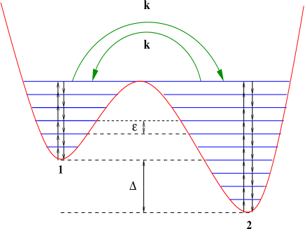
See Fig. 1 for a pictorial representation of the model. Each of the two wells, labeled $1$ and $2$, comprises a collection of $N_{i}~{}(i=1$ and $2$, respectively $)$ identical, non-interacting TLSs of such kind. For a collection of $N_{i}~{}(i=1,2)$ TLSs, a variable $\zeta_{j}^{i}(t),~{}(j=1,2,.....,N_{i})$ is defined, which takes on a value $0$ if at the given instant of time $t$ the level $0$ of the TLS $j$ is occupied and $1$ if otherwise. $\zeta_{j}^{i}(t)$ is thus an occupation variable. The variable $Q_{i}(t)~{}(i=1,2)$ is then defined as

$$Q_{i}(t)=\displaystyle\sum_{j=1}^{N_{i}}\zeta_{j}^{i}(t).$$ (6)

$Q_{i}(t)$, which serves to describe the level of instantaneous excitation in a collection of TLSs, is therefore a stochastic variable in the discrete integer space $[0,N_{i}]$. An $\alpha$ process occurs only when all the $\beta$ processes (TLSs) in a well are simultaneously excited, i.e., $Q_{i}=N_{i}$. There is a finite rate of transition $k$ from either wells when this condition is satisfied. Within the general framework of the model, the double-well becomes asymmetric when $N_{1}\neq N_{2}$.

Note that the double-well model has been widely used to describe relaxation in glassy liquids and we do not specify the microscopic nature of the two states any further. The main new ingredient we introduce is the condition that transition between the two wells is controlled by the collective variable $Q_{i}(t)$. Note also that the dynamics embodied in Fig. 1 is not the standard chemical dynamics in a bistable potential because the microscopic energy levels are in general degenerate. One should also note that in the energy landscape picture the transition from the initial state can occur to a limited number (but greater than unity) of final states.

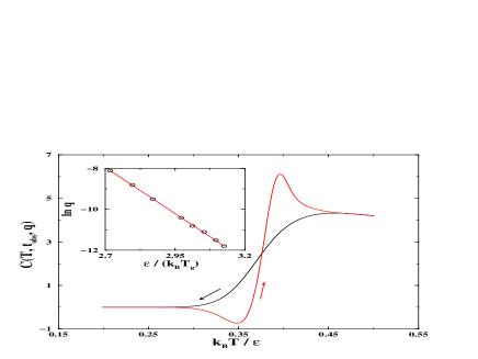
In Fig. 2, we show the heat capacity versus temperature $C-T$ curve obtained for our model. The curve looks very close to the ones observed in experiments.

Figure 2: The heat capacity versus reduced temperature plot for the system when subjected to a cooling-heating cycle with $q=7.5\times 10^{-5}$ in reduced units. The inset shows the plot of the logarithm of the cooling rate $q$ versus the reciprocal of the $T_{g}$. The slope of the linear fit to the data equals $-9.04$ in appropriate temperature units.

Note the sharp rise in heat capacity during heating. We now briefly describe the calculation procedure. The probability $P_{i}(n;T,t)$ that the stochastic variable $Q_{i}$ takes on a value $n$ at temperature T and time $t$ can be shown to satisfy the following stochastic master equation van Kampen :

$$\frac{\partial P_{i}(n;T,t)}{\partial t} = [(N_{i}-n+1)/\tau_{0}(T)]P_{i}(n-1;T,t)$$ (7)

$$+ [(n+1)/\tau_{1}(T)]P_{i}(n+1;T,t)$$

$$- [(N_{i}-n)/\tau_{0}(T)]P_{i}(n;T,t)$$

$$- (n/\tau_{1}(T))P_{i}(n;T,t)-k~{}\delta_{n,N_{i}}~{}P_{i}(n;T,t)$$

$$+ k~{}\delta_{n,N_{i\pm 1}}~{}\delta_{j,i\pm 1}~{}P_{j}(n;T,t),$$

where the ’$+$’ and ’$-$’ signs in the indices of the Kronecker delta are for $i=1$ and $2$, respectively. The total energy of the system at time $t$ can therefore be given by

$$E(T,t)=\displaystyle\sum_{n=0}^{N_{1}}P_{1}(n;T,t)~{}(N_{2}-N_{1}+n)~{}\epsilon+\displaystyle\sum_{n=0}^{N_{2}}P_{2}(n;T,t)~{}n~{}\epsilon,$$ (8)

where the lowest level of the well $2$ is taken to have zero energy. The set of equations, given by Eq. (7) for $n=0,1,...,N_{i}$ and $i=1,2$, is solved numerically by the matrix method, where the solution is expanded in terms of the eigenvectors and the eigenvalues of the transition matrix, and the coefficients of the expansion are evaluated from the initial distribution. Once we know $P_{i}(n;T,t)$, we can calculate the heat capacity $C$, as discussed below, from an equation, which is essentially a form of Eq. (2) modified to incorporate the nonequilibrium effects.

The system, when subjected to cooling or heating at a constant rate, can be envisaged to undergo a series of instantaneous temperature changes, each in discrete step of $\Delta T$ in the limit $\Delta T\rightarrow 0$, at time intervals of length $\Delta t$, whence $q=\Delta T/\Delta t$ Moynihan-JPC-1974 . A pictorial representation of the temperature control during a cooling process with finite $\Delta T$ was given by Jäckle Jackle . If we consider a time interval at the beginning of which the temperature has been changed from $T$ to $T^{\prime}=T+\Delta T$, the waiting time $t_{obs}$ before an observation can be made is restricted by $\Delta t$. The heat capacity $C$, measured at a time $t_{obs}$ subsequent to a temperature change from $T$ to $T^{\prime}=T+\Delta T$, is not stationary in time unless $t_{obs}$ is long enough for the equilibrium to be established. The measured heat capacity ( as is the energy ) then becomes a function of the rate of cooling / heating as well, apart from $T$ and $t_{obs}$. The dependence of $C$ on $q_{c}$ / $q_{h}$ implies that the measured heat capacity of a nonequilibrium state depends on the history of the preparation of that state. Here we restrict ourselves to the case, where $q_{c}=q_{h}=q$. We therefore calculate $C(T,t_{obs},q)$ from the following equation:

$$C(T,t_{obs},q)=\lim_{\Delta T\rightarrow 0}\frac{E(T+\Delta T,t_{obs},q)-E(T,0,q)}{\Delta T},$$ (9)

where the energies can be obtained from Eq. (8). In the present calculation, we have taken $t_{obs}=\Delta t$. Throughout the cycle the transition rates are assumed to be tuned with the heat bath temperature $T$.

Fig. 2 is the result of the model calculation where $N_{1}=6$ and $N_{2}=10$. Temperature $T$ is throughout expressed in reduced units of $\epsilon/k_{B}$ with $\epsilon$ taken to be unity. We have set $\Delta T=\pm 0.0015$ in reduced units. The correspondence to real units is discussed later. The model assumes the presence of an energy barrier for all the intra-well transitions. If $\epsilon^{\ddagger}_{i}$ be the energy barrier to the transition from the level $i$ in a TLS, the transition state theory (TST) allows one to write $\tau_{i}(T)=h/(k_{B}T)exp[\epsilon^{\ddagger}_{i}/(k_{B}T)]$, where $h$ is the Planck constant. Here we have set $\epsilon^{\ddagger}_{1}=8~{}\epsilon$. We express time also in reduced units, being scaled by $\tau_{1}(T_{h})$, where $T_{h}$ is the highest temperature considered in a cooling-heating cycle. Note that the cycle starts with the equilibrium population distribution at $T_{h}$. The inter-well transition rates are equal and independent of temperature. We have taken $k^{-1}=0.50$ in reduced time units. In order to further explore the merit of the model in reproducing the experimental results, we have investigated the cooling / heating rate dependence of $T_{g}$ for our model. The latter has been taken as the temperature of onset of the heat capacity increase as observed during heating Angell-Science-1995 . The $lnq$ versus $1/T_{g}$ plot, as shown in the inset of Fig. 2, is linear with negative slope in complete accordance with the experimental observations. The slope gives a measure of the energy of activation for the relaxation being in operation.

Figure 3: (a) Plot of the fictive temperature $T_{f}$ versus the heat bath temperature $T$ in reduced units for different cooling rates: $q=3.0\times 10^{-4},7.5\times 10^{-5},2.0\times 10^{-5},7.5\times 10^{-6}$ from top to bottom. The dashed line traces the $T_{f}=T$ line. The inset shows the dependence of the limiting fictive temperature $T^{L}_{f}$ obtained upon cooling on the rate of cooling. The slope of the linear fit to the data is $-9.13$ in appropriate temperature units. (b) The $dT_{f}/dT$ versus reduced temperature plot for the system with $N_{1}=6$ and $N_{2}=10$ when subjected to a cooling-heating cycles. The solid line is for $q=3\times 10^{-4}$, and the dashed line is for $q=7.5\times 10^{-5}$, both in reduced units. The inset shows the evolution of the energy of the system during a cooling-heating cycle with $q=7.5\times 10^{-5}$ in reduced units.

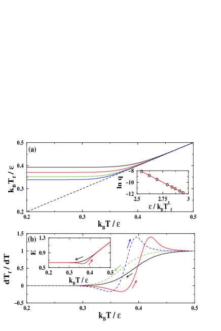
Fig. 3(a) shows a $T_{f}$ versus $T$ plot for different cooling rates, where the fictive temperature is calculated in terms of energy. The freezing of structural relaxation within the experimental time scale is evident from the attainment of a limiting fictive temperature. In the inset of Fig. 3(a), we show the plot of the logarithm of the cooling rate $q$ versus the reciprocal of the limiting fictive temperature $T^{L}_{f}$ obtained on cooling. The linearity of the plot with negative slope is again in excellent agreement with the experimental results. A plot of $dT_{f}/dT$ versus $T$ is displayed in Fig. 3(b) for two different cooling / heating rates. This is also in accord with the experimental observation.

So far we have presented the results in reduced units. It would be useful to have, at this point, an estimate of the real terms for reasonable input. For $\epsilon/k_{B}=600~{}K$, the cooling and heating rates explored here range from $0.0085$ to $0.35~{}Ks^{-1}$, while the temperature window we have looked into lies between $300~{}K$ and $120~{}K$. One should note that these rates are of the same order of magnitude as practised in experiments.

In order to probe the origin of the behavior of the calculated heat capacity, and also of $dT_{f}/dT$, during heating, we plot the energy $E$ versus the heat bath temperature $T$ during a cycle, as shown in the inset of Fig. 3(b). The fictive temperature evolves in an identical fashion as the energy. Note that the energy or the fictive temperature goes down during the initial period of heating before it starts increasing. The reason is as follows. The presence of an energy barrier for all the intra-well transitions results in a slow down of the elementary relaxation rates as the system is subjected to rate cooling. The system eventually gets trapped into a nonequilibrium glassy state on continued cooling. As one subsequently starts heating, the rate of the elementary relaxation increases, thus causing a delayed energy relaxation. This explanation further gains support from the calculated heat capacity being negative Odagaki-PRE-2001-2002 .

Figure 4: The heat capacity versus reduced temperature plot for the system with $N_{1}=3$ and $N_{2}=5$ when subjected to a cooling-heating cycle with $q=5\times 10^{-6}$ in reduced units. The inset shows the same plot for $q=1.5\times 10^{-4}$ in reduced units. The axis labels for the inset, being same as those of the main one, are not shown.

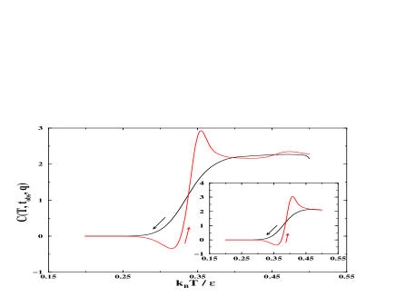
Fig. 4 shows a heat capacity versus temperature plot during a cooling-heating cycle for our proposed model obtained with a different set of parameters so chosen that the $\alpha$ relaxation becomes more probable within the observation time. A repeat of the non-monotonic pattern of the heat capacity, although in much smaller scale, is notable at higher temperatures during heating for slow cooling and heating. However, there has not been any report in the literature, to the best of our knowledge, of such an observation made experimentally. For faster rates, this repeat pattern vanishes as evident from the inset of Fig. 4. It is, therefore, reasonable to attribute this to the $\alpha$ relaxation.

A few comments regarding the present work are in order:
(1) The hysteresis in the $C$ versus $T$ plot, and also the overshoot of the heat capacity observed during heating, become progressively weaker as the cooling and heating rates decrease, and eventually vanish for sufficiently slow rates. This is again in agreement with the long known experimental results.
(2) While the elementary relaxation rates evolve with the heat bath temperature, it is the slow population relaxation that gives rise to the nonequilibrium effects.
(3) The relaxation of energy to its equilibrium value following a small temperature jump slows down rapidly as the temperature is lowered. This is due to the activated dynamics assumed here for transition between the two levels in a TLS. From the temperature variation of this relaxation time, one can have an estimate of the temperature where the system starts falling out of the equilibrium while cooling at a given constant rate.
(4) Our model, while simple and microscopic, is quite general and also detailed. Its success in reproducing all the aspects of experimental results on heat capacity during the cooling-heating cycle is noteworthy. Another important aspect is that we need not invoke any singularity, thermodynamic or kinetic, to explain the anomalies. It is worth mentioning here that a similar model can describe many aspects of nonexponential relaxation observed in glassy liquids Chakrabarti-Bagchi . We are currently investigating the relationship of the heat capacity anomaly with the fragility of the system Angell .

We thank Mr. R. Murarka for several helpful discussions. This work was supported in parts by grants from CSIR and DST, India. DC acknowledges the University Grants Commission (UGC), India for providing the Research Fellowship.

References

- (1) C. A. Angell, K. L. Ngai, G. B. McKenna, P. F. McMillan and S. W. Martin, J. Appl. Phys. 88, 3113 (2000).
- (2) M. D. Ediger, C. A. Angell and S. R. Nagel, J. Phys. Chem. 100, 1322 (1996).
- (3) P. G. Debenedetti and F. H. Stillinger, Nature 410, 259 (2001).
- (4) C. T. Moynihan, A. J. Easteal, J. Wilder, and J. Tucker, J. Phys. Chem. 78, 2673 (1974).
- (5) C. T. Moynihan, A. J. Easteal, M. A. DeBolt, and J. Tucker, J. Am. Ceram. Soc. 59, 12 (1976).
- (6) M. A. DeBolt, A. J. Easteal, P. B. Macedo, and C. T. Moynihan, J. Am. Ceram. Soc. 59, 16 (1976).
- (7) J. H. Gibbs and E. DiMarzio, J. Chem. Phys. 28, 373 (1958).
- (8) X. Xia and P. G. Wolynes, Proc. Natl. Acad. Sci. U. S. A. 97, 2990 (2000).
- (9) N. O. Birge and S. R. Nagel, Phys. Rev. Lett. 54, 2674 (1985).
- (10) D. Oxtoby, J. Chem. Phys. 85, 1549 (1986).
- (11) A. Tool and C. G. Eichlin, J. Am. Ceram. Soc. 14, 276 (1931).
- (12) B. Halpern and J. Bisquert, J. Chem. Phys. 114, 9512 (2001).
- (13) S. A. Brawer, Relaxation in Viscous Liquids and Glasses (McGraw-Hill, New York, 1983).
- (14) S. A. Brawer, J. Chem. Phys. 81, 954 (1984).
- (15) J. Jäckle, Rep. Prog. Phys. 49, 171 (1986).
- (16) T. Tao, A. Yoshimori, and T. Odagaki, Phys. Rev. E 64, 46112 (2001); 66, 41103 (2002).
- (17) F. H. Stillinger, Science 267, 1935 (1995).
- (18) S. Sastry, P. G. Debenedetti, and F. H. Stillinger, Nature 393, 554 (1998).
- (19) M. Pollak and G. E. Pine Phys. Rev. Lett. 28, 1449 (1972).
- (20) K. S. Gilroy and W. A. Phillips, Philos. Mag. B 43, 765 (1981).
- (21) U. Buchenau, Phys. Rev. B 63, 104203 (2001).
- (22) N. G. van Kampen, Stochastic Processes in Physics and Chemistry (Elsevier Science B. V., Amsterdam, 1992).
- (23) C. A. Angell, Science 267, 1924 (1995).
- (24) D. Chakrabarti and B. Bagchi, cond-mat/0303151.
- (25) C. A. Angell, J. Non-Cryst. Solids 131-133, 13 (1991); L. -M. Wang, V. Velikov, and C. A. Angell, J. Chem. Phys. 117, 10184, 2002.