Applications of Ideas from Random Matrix Theory
to Step Distributions on “Misoriented” Surfaces

Abstract

Arising as a fluctuation phenomenon, the equilibrium distribution of meandering steps with mean separation $\langle\ell\rangle$ on a “tilted” surface can be fruitfully analyzed using results from RMT. The set of step configurations in 2D can be mapped onto the world lines of spinless fermions in 1+1D using the Calogero-Sutherland model. The strength of the (“instantaneous”, inverse-square) elastic repulsion between steps, in dimensionless form, is $\beta(\beta-2)/4$. The distribution of spacings $s\langle\ell\rangle$ between neighboring steps (analogous to the normalized spacings of energy levels) is well described by a “generalized” Wigner surmise: $p_{\beta}(0,s)\approx as^{\beta}\exp(-bs^{2})$. The value of $\beta$ is taken to best fit the data; typically $2\leq\beta\leq 10$. The procedure is superior to conventional Gaussian and mean-field approaches, and progress is being made on formal justification. Furthermore, the theoretically simpler step-step distribution function can be measured and analyzed based on exact results. Formal results and applications to experiments on metals and semiconductors are summarized, along with open questions. (conference abstract)

I Introductory Synopsis

For over a decade we have studied the correlation functions of steps on vicinal surfaces of crystals, that is to say crystals that are intentionally misoriented from high-symmetry directions. Of special experimental interest is the distribution of separations of adjacent steps, corresponding to $p_{\beta}(0,s)$ of random matrix theory MehtaRanMat . Traditionally, surface scientists have described it by a Gaussian, with a controversy arising about the relationship between the width of the Gaussian and the strength of the repulsion between steps. This controversy is resolved, and a better representation of the step distribution obtained, by characterizing the problem with the Calogero-Sutherland models and using the simple expression of the Wigner surmise, with [seemingly for the first time] general values of $\beta$ in the range of 2 to 10. This range is rarely considered by random-matrix theorists. The step-step correlation function resulting from the Calogero-Sutherland models, for which exact but numerically intractable solutions exist, can also be applied to data.

II Background

On vicinal crystals there are a sequence of terraces oriented in the high-symmetry direction and separated by steps typically one atomic layer high. If the spacing between adjacent steps (the “terrace width”) is denoted $\ell$, then the mean spacing $\langle\ell\rangle$ is 1/$\tan\phi$, where $\phi$ is the angle by which the surface is tilted from the high-symmetry direction. For theoretical modeling it is convenient to think of the crystal as being a simple cubic lattice. (The extension to realistic symmetries is not difficult but muddies the discussion.) By [“Maryland”] convention, the steps run on average in the $\hat{y}$ direction, so that the step spacings $\ell$ are in the $\hat{x}$ direction. (The high-symmetry terrace plane is then $\hat{z}$.) For metals it is a decent approximation to take the total energy of the system to be proportional to the number of nearest neighbor bonds. (For semiconductors corner energies can play a role, but these are insignificant for the properties discussed in this paper.) Then the ground-state configuration is a set of perfectly straight steps (uniformly spaced because of repulsions we shall discuss shortly). At low temperatures, the predominant excitation are kinks in the steps, each costing energy $\epsilon$. At higher temperatures, atoms and vacancies appear on the terraces (each with energy 4$\epsilon$ in the simple model), but these are neglected here. The resulting model is called the terrace-step-kink model (TSK) or terrace-ledge-kink model in the literature.

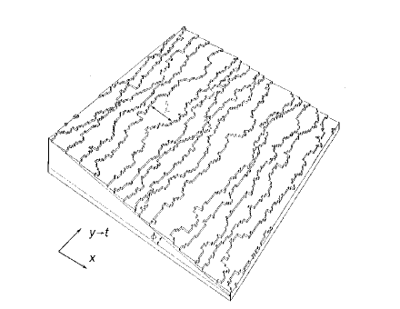
Figure 1: Illustration of a vicinal generated by a Monte Carlo simulation of the terrace-step-kink (TSK) model, showing that the elementary thermal excitation is the kink, a unit excursion of a step in the $x$ direction. (Adapted from Fig. 1 of Ref. 27) For experimental STM (scanning tunneling microscopy) images of a vicinal surface; see, e.g., Fig. 1 of Ref. 12, Fig. 1 of Ref. 15, and Fig. 1 of Ref. 34. In the Gruber-Mullins approximation, only one step meanders, the others being straight along the $y$ direction and uniformly spaced. (Cf. Fig. 9 of Ref. 12.) In the fermion picture, the $y$ direction is viewed as time-like. In the step continuum model, the steps meander continuously rather than by discrete deviations (i.e., the kinks are smoothed).

In this low-temperature picture, the number of steps is fixed (by the miscut angle in an experiment and by screw periodic boundary conditions in a numerical simulation). Thus, the steps never start or stop, and they all have the same orientation (say up): there are no anti-steps (or down-steps). It is convenient and fruitful to imagine the $\hat{y}$ direction as time-like and to view the configurations of steps as the worldlines of a collection of a single kind of particle in one spatial dimension (viz. $\hat{x}$) evolving in time. For physical reasons, the steps cannot cross each other (since that would involve atoms suspended above the terrace held with just a couple lateral bonds). Assuming also that the steps cannot merge to form double-height steps, we can view the evolving 1D particles as spinless fermions. (Equivalently, in 1D, they can be treated as hard bosons, a viewpoint exploited in a study of step bunching szs . Moreover, the system is highly reminiscent of soliton lines in 2D incommensurate crystals pt .)

The obvious next question is how these spinless fermions interact. A typical way to characterize the distribution of steps is by their terrace-width distribution (TWD), i.e. the probability of finding the next step a distance $\ell$ away. This probability distribution is denoted $P(s)$, where $s\equiv\ell/\langle\ell\rangle$ denotes the step spacing normalized by the [only] characteristic length in the $\hat{x}$ direction. By construction, $P(s)$ is normalized and has unit mean. (It ultimately corresponds to $p(0,s)$ of random-matrix theory.) For the ground state, $P(s)$ is essentially a delta function at $s$=1. If the steps are imagined as straight (“uncooked spaghetti”) and deposited randomly with probability 1/$\langle\ell\rangle$, then $P(s)$ becomes exp(-$s$). In fact, however, at finite temperature the steps do meander, leading to well-known entropic (or steric) repulsion due to the underweighting in the partition function of steps on the verge of crossing. This effect is particularly noticeable as $s$ approaches 0: $P(s)$ now vanishes with power-law behavior rather than growing to unity. For $s\gg 1$ $P(s)$ must decay faster than exp(-$s$) to preserve the unit mean; analogies with random walkers suggest exp(-$bs^{2}$) as the form of the tail MEF . There are many arguments to show that the entropic repulsion per length is proportional to $(k_{B}T)^{2}/\tilde{\beta}\ell^{2}$; here the step stiffness $\tilde{\beta}\equiv\beta(\theta)+d^{2}\beta/d\theta^{2}$, with [orientation-dependent] free energy per length conventionally called $\beta(\theta)$ in surface studies.

In addition to the entropic repulsion, there generally is an elastic interaction, also having the inverse-square form $A/\ell^{2}$, due to repulsion between force dipoles intrinsic to the steps Rickman ; mp : Viewed from a continuum picture, the step involves a pair of sharp angles which could lower their energy by healing to form more obtuse angles. This process leads to a strain field around the step in which atoms in the terraces bounding the step (both above and below) tend to move away from the step. Atoms between two steps are then frustrated since they are pushed in opposite directions by the pair of steps. Thus, they cannot relax fully, leading effectively to a repulsion, with $A$ proportional to the product of the step dipoles.

In the fermion picture, the strength of the elastic repulsion only enters in the dimensionless combination

$$\tilde{A}\equiv\tilde{\beta}A/(k_{B}T)^{2}.$$ (1)

The elastic and entropic repulsions do not simply add together: As the strength $A$ of the elastic interaction increases, the chance of steps coming near each other decreases, thereby reducing the entropic repulsion. Hence, the dimensionless strength of the inverse square repulsion in essence ftntpsq6 becomes WmsErr ; CL

$$\tilde{A}\rightarrow\frac{1}{4}\left[1+\sqrt{1+4\tilde{A}}\right]^{2}\,.$$ (2)

In situations where the surface has a metallic surface state [one which crosses the Fermi energy], there can also be an oscillatory [in sign] interaction between steps, albeit with a 1/$\ell^{2}$ envelope RZ92 ; TLE-U . Such an interaction destroys many of the scaling properties, particularly that the form of $P(s)$ is well defined, i.e. that plots of $\langle\ell\rangle\hat{P}(\ell)$ vs. $\ell/\langle\ell\rangle$ are independent of $\langle\ell\rangle$. Further discussion of this digression is beyond the scope of this paper.

Knowledge of the elastic strength $A$ is crucial to adequate characterization of a stepped surface. It is one of just three parameters (the stiffness $\tilde{\beta}$ being another) of the widely-applied step continuum model JW99 and underlies the “2D pressure”, which determines surface morphology (e.g., whether steps “bunch”) and drives kinetic evolution. It is generally believed that the repulsions can be adequately approximated as acting between pairs of steps at the same value of $y$, i.e. instantaneously in the 1D fermion representation. This approximation is clearly crucial for viability of the fermion approach.

The simplest way to estimate $P(s)$ was developed over a third of a century ago. In treating polymers in 2D, deGennes pointed that the energy of a step (or a polymer) could be described as the line integral over path-length ingrements times $\beta(\theta)$. Expanding to lowest order, we get a constant (the straight step) plus what amounts to a kinetic energy proportional to $\tilde{\beta}\,(dx/dy)^{2}$, the mass-like stiffness times the 1D velocity squared.

In the mean-field (i.e. single active step with all others fixed at spacings $\langle\ell\rangle$) approximation Gruber67 , Gruber and Mullins (GM) reduced the “free fermion” case ($A$=0) to the familiar elementary quantum mechanics problem of solving the Schrödinger equation for a spinless fermion of mass $\propto\tilde{\beta}$ in a hard-wall box of length 2$\langle\ell\rangle$. The probability density of the ground state (the squared ground-state wavefunction) is just $P_{GM-0}(s)=\sin^{2}(\pi s/2)$, for $0\leq s\leq 2$; remarkably, the associated ground-state energy is precisely the entropic repulsion. For $\tilde{A}$ above about 3/2, the problem becomes that of a particle in a parabolic potential, i.e. a simple harmonic oscillator, giving $P_{GM}\propto\exp[-(s-1)^{2}/2w_{GM}^{2}]$, with $w_{GM}\propto\tilde{A}^{-1/4}\langle\ell\rangle$ Bartelt90 . These parametric results were dramatically verified for Si(111): not only was the TWD measured at one misorientation well fit by a Gaussian, but the TWD at a second misorientation was well described by another Gaussian whose width was simply rescaled by the change in $\langle\ell\rangle$, with $no$ refitting WangWms ; Metois .

However, the Grenoble group pointed out a flaw in Gruber-Mullins approach in the limit of very strong $\tilde{A}$ IMP98 . There the entropic repulsion becomes negligible and the steps can be imagined as meandering independently (albeit by a small amount). Then the variance of the TWD should not be just $w_{GM}^{2}$, but twice that amount, since both steps bounding a terrace are meandering. (The actual increase is less than two-fold due to lingering anticorrelations.) Hence, a fit of the TWD width in the Gruber-Mullins approximation would underestimate $\tilde{A}$ by a factor of over 3 in the limit of very large $\tilde{A}$. Based on roughening theory, the Saclay group Barbier concluded that the underestimate, for more general $\tilde{A}$, was somewhat smaller (about 2).

Meanwhile, Ibach noted that the TWD of the free-fermion distribution could be far better approximated by an expression $\propto s^{2}\exp(-bs^{2})$, in essence the Wigner surmise for free fermions, than by $P_{GM-0}(s)=\sin^{2}(\pi s/2)$. How this comes about becomes evident by recasting the preceding model in terms of the celebrated CGbook Calogero-Sutherland models C69 ; Suth71Cal ; Suth71Suth .

III Connection to Random Matrix Theory via Calogero-Sutherland Models

In his study of the spacings of energy levels in nuclei, Wigner’s starting inspiration was to consider ensembles of dynamical systems governed by different Hamiltonians with common symmetry properties Guhr98 . The three generic Hamiltonian symmetries are orthogonal, unitary, and symplectic. The key ingredient is level repulsion: two states connected by a non-vanishing matrix elements repel each other by an amount determined by the symmetry of the Hamiltonian. While inapplicable to average quantities, the approach is appropriate for the fluctuation of a large number of energy levels. These fluctuations should become independent of the specifics of the level spectrum and the weight factors, and so should exhibit a universal form depending only on symmetry. This idea can also be derived from maximum-entropy arguments Guhr98 .

One can draw a correspondence between the fluctuations of energy spacings between adjacent energy levels in nuclei and the fluctuations of spatial separations between adjacent fermions in 1D systems. (In other chaotic systems, as well, there is a correspondence between energy and spatial spacings.) The Calogero-Sutherland model describes spinless fermions in 1D which interact via an inverse square potential. Specifically, Sutherland’s version Suth71Cal of the Calogero Hamiltonian C69 for the fluctuations of uniformly-spaced fermions on an infinite line is:

$${\cal H}_{\rm CS}=-\sum_{j=1}^{N}\frac{\partial^{2}}{\partial x_{j}^{2}} + 2\frac{\beta}{2}\left(\frac{\beta}{2}-1\right)\sum_{1\leq i<j\leq N}(x_{j}-x_{i})^{-2}$$ (3)

$$+ \omega^{2}\sum_{j=1}^{N}x_{j}^{2},$$

in the limits $N\rightarrow\infty$ and $\omega\rightarrow 0$. (In Calogero’s original model C69 , the last term ($\propto\omega^{2}$) is summed over particle separations $(x_{j}-x_{i})^{2}$ rather than deviations from integer positions $x_{j}^{2}$.) The ground-state wavefunction for this Hamiltonian is

$$\Psi_{0}=\prod_{1\leq i<j\leq N}\left|x_{j}-x_{i}\right|^{\beta/2}\exp\left(-\frac{1}{2}\omega\sum_{k=1}^{N}x_{k}^{2}\right)$$ (4)

The ground-state density $\Psi_{0}^{2}$ is recognized as a joint probability distribution function from the theory of random matrices for Dyson’s Gaussian ensembles Dyson69 .

The Sutherland HamiltonianSuth71Suth similarly describes spinless fermions on a circle of radius $L$ (with $L\rightarrow\infty$), having inverse-square interactions along chords:

$${\cal H}_{\rm S}=-\sum_{j=1}^{N}\frac{\partial^{2}}{\partial x_{j}^{2}}+2\frac{\beta}{2}\left(\frac{\beta}{2}-1\right)\frac{\pi^{2}}{L^{2}}\sum_{i<j}\left[\sin\frac{\pi(x_{j}-x_{i})}{L}\right]^{-2}$$ (5)

In this case the ground-state wavefunction has the Jastrow form

$$\Psi_{0}=\prod_{i<j}\left|\sin\frac{\pi(x_{j}-x_{i})}{L}\right|^{\beta/2},\quad x_{j}>x_{i}$$ (6)

With the definition $\theta_{i}\equiv 2\pi x_{i}/L$, the ground-state density $\Psi_{0}^{2}$ can be written as

$$\Psi_{0}^{2}=\prod_{i<j}\left|e^{i\theta_{j}}-e^{i\theta_{i}}\right|^{\beta}$$ (7)

This ground-state density is again a joint probability distribution function from the theory of random matrices, now for Dyson’s circular ensembles Dyson62 .

From Eqs. (3) and (5), the dimensionless interaction $\tilde{A}$ can be identified as $(\beta/2)(\beta/2-1)$. Conversely, $\beta$ is just the quantity inside the brackets in expression (2). These models can be solved exactly only for the special cases $\beta$ = 1, 2, or 4, corresponding to orthogonal, unitary, or symplectic symmetry of the ensemble. In the literature of random matrix theoryMehtaRanMat , the TWD $P(s)$ is often denoted $p(0,s)$, the probability of finding two levels separated by $s$ with zero intervening levels. Note also that $\beta$ was used in the previous section to denote the step free energy per length. (Presumably the letter was chosen to emphasis the similarity to but difference from the surface free energy per area $\gamma$.) Dyson Dyson62 ; MehtaRanMat chose $\beta$ to denote this exponent to indicate the analogy to an inverse temperature (of a Coulomb gas on a circle). While we follow this convention here to minimize the chance of confusion, in our applications to stepped surfaces the exponent is called $\varrho$ to minimize confusion for that audience. (The stiffness $\tilde{\beta}$ is essentially unrelated to the exponent $\beta$!)

Random matrix theory leads to exact solutions for the ground state properties of the three special cases, in particular for $P(s)$. There are even prescriptions that allow one to generate numerical representations of arbitrary accuracy Dyson70 ; Joos91 . However, these expressions involve terms in a series and are not useful for fitting experimental data. Wigner surmised that $P(s)$ has the simple form

$$P_{\beta}(s)=a_{\beta}s^{\beta}e^{-b_{\beta}s^{2}}$$ (8)

for the special cases $\beta$= 1, 2, and 4. The constants $a_{\beta}$ associated with normalization of $P(s)$ and $b_{\beta}$ producing unit mean are:

$$a_{\beta}=\frac{2\left[\Gamma\left(\frac{\beta+2}{2}\right)\right]^{\beta+1}}{\left[\Gamma\left(\frac{\beta+1}{2}\right)\right]^{\beta+2}}\quad\mbox{and}\quad b_{\beta}=\left[\frac{\Gamma\left(\frac{\beta+2}{2}\right)}{\Gamma\left(\frac{\beta+1}{2}\right)}\right]^{2}\,.$$ (9)

From Eq. (8) one can readily find analytic expressions for the moments and other measurable properties of $P(s)$ EP99 .

The argument for Eq. (8) focusses on the Jacobean associated with a change of variables for the Gaussian-ensemble probability distribution function $p({\cal H})\sim\exp[-bN\,{\rm tr}({\cal H}^{2})]$ from the eigenenergies to the combinations of the matrix elements. For an orthogonal ensemble ($\beta$=1) with $N$=2, the integrand has a Dirac delta function with argument $s-[(h_{11}-h_{22})^{2}+4h_{12}^{2}]^{1/2}$, which vanishes for $s$=0 only when the two [squared] independent variables do. Hence, $P(s)\propto s$, corresponding to a circular shell in parameter space and leading to $\beta$=1. For unitary ensembles there is an additional independent parameter since $h_{12}^{2}$ becomes $(\Re{\rm e}\,h_{12})^{2}+(\Im{\rm m}\,h_{12})^{2}$. Hence, $P(s)\propto s^{2}$, corresponding to a spherical shell in parameter space, i.e. $\beta$=2. Exact for $N$=2, these arguments are still fine guides for large $N$ Zwer98 : As seen most clearly by explicit plots as in Haake’s text Haake91 , $P_{1}(s)$, $P_{2}(s)$, and $P_{4}(s)$ are excellent approximations of the exact results for orthogonal, unitary, and symplectic ensembles, respectively, and these simple expressions are routinely used when confronting experimental data Guhr98 ; Haake91 . (The agreement is particularly impressive for $P_{2}(s)$ and $P_{4}(s)$, which are germane to stepped surfaces.) Furthermore, Eq. (8) has a similar variance at very large $\beta$ to that predicted by the Grenoble group, and more generally approaches the form of a Gaussian for $\beta$ not too smallERCP01 .

Figure 2: $P(s)$ vs. $s\equiv\ell/\langle\ell\rangle$ for the exact “free-fermion”, $\tilde{A}$=0 result (solid curve), the Gruber-Mullins approximation $\sin^{2}(\pi s/2)$(long-short dashed curve), and the $\beta$=2 Wigner surmise (Eq. (8)) result (dotted curve), barely distinguishable from the exact result). Offset upward by 0.4 for clarity, an analogous plot of the exact result for $\tilde{A}$=2, the Gruber-Mullins Gaussian approximation $(24/\pi^{2})^{1/4}\exp(-\surd 24(s-1)^{2})$ (long-short dashed curve), and the $\beta$=4 Wigner surmise result (dotted curve). (Adapted from Fig. 1 of Ref. 31).

The essential innovation in our work is the conjecture that the generalized Wigner surmise expressed in Eq. (8) for arbitrary values of $\beta$ provides a good approximation for these non-special values. For these general values, there is no recourse to formal justification from symmetry arguments. (Indeed, it remains mysterious whether there is some deep underlying reflection of the random-matrix symmetry and the corresponding Calogero-Sutherland models at the special values of $\beta$.) The only way to test our hypothesis is to generate numerical data. This task has occupied us for some time. We have used both Monte Carlo and transfer matrix computations of TSK models ERCP01 ; HCRE . The details of these studies are beyond the scope of this paper, but the main result is that the generalized Wigner surmise does better than any of the earlier Gaussian approximations in accounting for the dependence of the TWD’s variance—the quantity typically measured by experimentalists—on the value of $\tilde{A}$. In particular, the numerical data confirms that the proportionality coefficient between the width $w$ of the TWD and $\tilde{A}^{-1/4}$ (or more accurately, between $w$ and $\beta^{-1/2})$ is not constant but increases slowly with $\tilde{A}$.

Obtaining the experimentally measurable variance $\sigma^{2}$ of $P(s)$—essentially $w^{2}$ when the Gaussian approximation is viable—analytically from Eq. (8), weRCEG can use a series expansion to derive an excellent estimate of $\tilde{A}$ from $\sigma^{2}$:

$$\tilde{A}\approx\frac{1}{16}\left[(\sigma^{2})^{-2}-7(\sigma^{2})^{-1}+\frac{27}{4}+\frac{35}{6}\sigma^{2}\right]\,,$$ (10)

with all four terms needed to provide a good approximation over the full physical range of $\tilde{A}$, from near zero up to around 16, corresponding to $\beta$ ranging from 2 up to about 8. The Gaussian methods described earlier essentially use just the first term of Eq. (10) and adjust the prefactor.

We have successfully applied these ideas (both direct fits to Eq. (8) and use of Eq. (10)) to experimental data by several different groups ERCP01 , focussing primarily on extensive results for vicinal Cu (001) and (111) obtained by Giesen, Ibach, and collaborators at FZ-Jülich RCEG ; Giesen00 .

IV Pair Correlation Functions

While the TWD is usually the easiest quantity to measure, it is generally not the easiest to calculate since it is essentially a many-body correlation function due to the demand that there be no fermion between the two fermions separated by $\ell$ (or $s$). The pair correlation function $h(s)$ (also called $1-Y(s)$ in random-matrix literatureMehtaRanMat ) indicates the probability of finding a fermion a normalized distance $s$ from a reference fermion, regardless of whether there are any between them. For a “perfect staircase” this would just be a set of delta functions at positive integers. More generally, $h(s)$ increases like $s^{\beta}$ for $s\ll 1$ just like $P(s)$. There are then a sequence of peaks at integer values of $s$ with dips between them. The amplitude of the crests and troughs relative to the mean density of fermions decreases as $s$ increases. For most purposes, but not here, it suffices to use the harmonic approximation KO82 ; SB99 ; Forres92 (which is essentially similar to the Grenoble approximation):

$$\langle\ell\rangle h_{\beta}(s) = \sum_{m\neq 0}(B_{m}\pi)^{1/2}\exp[-B_{m}(s-m)^{2}];$$ (11)

$$\frac{\pi^{2}\beta}{4B_{m}}=\gamma\! + \!\log(2\pi m)\!-\!{\rm ci}(2\pi m)=\sum_{j=1}^{\infty}(-1)^{j+1}\frac{(2\pi m)^{2j}}{2j(2j)!},$$

where $\gamma\simeq 0.577$ is Euler’s constant and ci is the cosine integral. Note that $B_{m}$ is proportional to $\beta$, so that peaks become sharper and higher with increasing repulsion. Also, $B_{m}$ decreases slowly but monotonically with increasing $m$. While useful for many applications KO82 ; SB99 ; Forres92 , this approximation for $h_{\beta}(s)$ proved inadequate for deducing $\beta$ from data.

Forrester Forres92 found an exact solution for even values of $\beta$. This expression, which involves Selberg correlation integrals, takes nearly a page of text, so is not reproduced here. We do note that the ratio of the exact prefactor of $s^{\beta}$ in $h_{\beta}(s)$ to $a_{\beta}$ in $P_{\beta}(s)$ is close to unity, lending further support to the utility of the generalized Wigner surmise expression ftntharatio .

Subsequently, Ha and Haldane HH ; h94 ; Les derived an exact solution for any rational value of $\beta$. In principle, this result also contains information about the “dynamic” correlations between fermions (i.e. between steps at different values of $y$). Unfortunately, their expression is even longer than that of Forrester, and so also is not reproduced here. Moreover, it seems to be numerically intractable, so of little “practical” use.

Fortunately, Gangardt and Kamenev GK01 recently derived the following asymptotic expansion for $h(s)$:

$$\langle\ell\rangle h_{\beta}(s) \sim -\frac{1}{\pi^{2}\beta s^{2}}+2\sum_{j=1}^{\infty}\frac{d_{j}^{2}(\beta)}{(2\pi s)^{4j^{2}/\beta}}\cos(2\pi js);$$ (12)

$$d_{j}(\beta)= \Gamma \!\!\!\!\!\!\left(\!1+\frac{2j}{\beta}\right)\prod_{m=1}^{j-1}\left(\frac{2m}{\pi\beta}\right)\sin\!\left(\frac{2\pi m}{\beta}\right)\Gamma^{2}\!\!\left(\frac{2m}{\beta}\right).$$

This formula turns out, remarkably, to be useful well below the asymptotic limit, and provides a good approximation—much better than the harmonic approximation—for $s>1/2$; it can be patched onto $a_{\beta}s^{\beta}$ for $s\leq 1/2$.

In confronting data with Eq. (IV), one must beware the limited number of steps in experimental images. In our application CohenSchr , there were only about a half dozen steps per image. Hence, we included an ad hoc linear decay envelope to account for this limit on $h(s)$ at large $s$. The system in question involved steps on Si(111) at very high temperatures, necessitating a clever device to compensate for evaporation. For a variety of reasons, the difficulty of the measurement led to data that presented exceptional challenges for analysis. One problem was that steps sometimes disappeared from the image, leading to the concern that the TWD might appear wider than it in fact was (since sometimes second-neighbor spacings rather than adjacent ones might be counted). The investigation showed that electromigration from the current which heated the sample tended to keep the steps apart, leading to correlation functions indicative of a larger [effective] $\tilde{A}$ than predicted from extrapolation of results at lower temperature.

V Concluding Comments

We have seen that steps on misoriented surfaces can be represented by fluctuating spinless fermions in 1+1D. Thus, step-step correlation functions can be expressed in terms of the Calogero-Sutherland model and thereby related to random matrix theory. In particular, the terrace width distribution, identified as a joint probability distribution, can be well described by the generalized Wigner surmise, evidently not only for the special cases related to orthogonal, unitary and symplectic ensembles but for arbitrary fermion repulsion strength. While perhaps reminiscent of some interpolation schemes, such a generalization has not, to my knowledge, been made before. Furthermore, most of these interpolation schemes have involved systems with mixed symmetries (typically orthogonal and unitary), with values of $\beta$ between 1 and 2 (and also between 0 and 1, where $\beta$=0 indicates Poissonian [random “uncooked spaghetti”] behavior). For stepped surfaces the physically interesting range starts near $\beta$=2 and goes past 4 up to 8 or even 10. This range has received minimal (if any) theoretical attention.

While the discovery of exact solutions is always intellectually exciting and captivating, they are often of little use in confronting experiments—physical or numerical—unless the formulas are numerically tractable. Thus, even when a problem is formally solved, neither theoreticians or funding agencies should view it as completed until the formalism can be rendered in a way that allows the extraction of numbers, even if approximately.

A major open question is the “deeper meaning” of the generalized Wigner surmise of Eq. (8), since there is no evident symmetry to argue for the simple expression. Howard Richards has taken the lead in trying to derive this result from an effective Hamiltonian beyond . This approach should lead to the development of the form of $P(s)$ for systems with higher-order terms in the repulsion potential and even potentials with an oscillatory term such as when metallic surface states mediate the interaction. (In systems in which “non-instantaneous” interactions (in directions other than $\hat{x}$ are significant, the usefulness of the mapping to 1D fermions is likely to break down.) It will be interesting to see whether expressions similar to the generalized Wigner surmise arise in other areas of physics. For example, while considering the probability distribution of stock market returns in the Heston model with stochastic volatility (in econophysics research), Yakovenko showed that the probability distribution of the variance—which is derived from a Fokker-Planck equation, has the form of the generalized Wigner surmise DY02 ! (In this case the value of $\beta$ was 1.6, so in a different regime from stepped surfaces.

While Eq. (8) assumes that $s$ is continuous, experiments and numerical simulations involve discrete lattices. We have shown ERCP01 ; HCRE ; RCEG that so long as $\langle\ell\rangle$ is at least 4 lattice spacings, there are no significant complications due to discreteness and that assuming continuous $s$ does not distort the analysis. In particular, the roughening transition to a facet that occur for discrete lattices Barbier ; VGL does not happen in the range of physical parameters HCRE .

Another skirted issue concerns how many steps interact. While the entropic interaction ipso facto involves just adjacent steps, the Calogero-Sutherland models C69 ; Suth71Cal ; Suth71Suth and the Saclay approach Barbier assume energetic interactions between all steps. The Gruber-Mullins Gruber67 ; Bartelt90 and Grenoble IMP98 ; EP99 approximations allow all steps or just adjacent ones to interact. Most Monte Carlo and transfer matrix simulations assume that just adjacent steps interact. In the Gruber-Mullins approximation, the curvature of the potential involves the inverse 4th power of the distance from neighboring steps, so that the effective strength of the repulsion increases by $\zeta(4)=\pi^{4}/90\approx 1.08$ when interactions between all steps rather than just adjacent ones are included ERCP01 ; in the Grenoble approximation it increases by about 1.10. These changes are relatively small, but the good agreement is curious between the variance predicted by Eq. (8) and our Monte Carlo results with just adjacent steps interacting HCRE .

For surface scientists a fundamental objective is to show consistency between the value of $A$ deduced from the TWD and that predicted from surface stress using Marchenko’s formula mp . However, most experimental systems do no possess the elastic isotropy assumed by that classic result. Hence, this goal has been elusive.

Another interesting problem is what happens when the mean direction of the steps (i.e. $\hat{y}$) does not correspond to a high-symmetry direction of the surface. We have recently found that the stiffness computed from standard near-neighbor bond lattice models (Ising or SOS models) underestimates the experimentally observed stiffness by a factor of about 4 for the square-net face of copper DGIE . The most likely explanations are significant long-range interactions or perhaps local relaxations leading to 3-atom effects. Furthermore, it is by no means obvious that the assumption of only “instantaneous” interactions between steps is justifiable for substantial azimuthal misorientation.

References

- (1) M.L. Mehta, Random Matrices, 2nd ed. (Academic, New York, 1991).
- (2) V.B. Shenoy, S.W. Zhang, and W.F. Saam, Phys. Rev. Lett. 81, 3475 (1998); Surface Sci. 467, 58 (2000).
- (3) V.L. Pokrovsky and A.L. Talapov, Theory of Incommensurate Crystals (Harwood Academic, New York, 1984).
- (4) M.E. Fisher, J. Stat. Phys. 34, 667 (1984) and pvt. comm.
- (5) J.M. Rickman and D.J. Srolovitz, Surface Sci. 284, 211 (1993).
- (6) V.I. Marchenko and A.Ya. Parshin, Sov. Phys. JETP 52, 129 (1980).
- (7) There is an additional overall factor of , so that the combined repulsion is WmsErr ; CL .
- (8) C. Jayaprakash, C. Rottman, and W.F. Saam, Phys. Rev. B 30, 6549 (1984); E.D. Williams, R.J. Phaneuf, J. Wei, N.C. Bartelt, and T.L. Einstein, Surface Sci. 310, 451 (1994).
- (9) See P.M. Chaikin and T.C. Lubensky, Principles of Condensed Matter Physics (Cambridge Univ. Press, Cambridge, 1995), chap. 10.5.1, and references therein, for general background.
- (10) A.C. Redfield and A. Zangwill, Phys. Rev. B 46, 4289 (1992).
- (11) T.L. Einstein, in: Handbook of Surface Science, vol. 1, W.N. Unertl, ed. (Elsevier Science B.V., Amsterdam, 1996), chap. 11.
- (12) H.-C. Jeong, E.D. Williams, Surf. Sci. Rep. 34, 171 (1999).
- (13) E.E. Gruber and W.W. Mullins, J. Phys. Chem. Solids 28, 875 (1967).
- (14) N.C. Bartelt, T.L. Einstein, and E.D. Williams, Surface Sci. 240, L591 (1990).
- (15) X.-S. Wang, J.L. Goldberg, N.C. Bartelt, T.L. Einstein, and E.D. Williams, Phys. Rev. Lett. 65, 2430 (1990).
- (16) C. Alfonso, J.M. Bermond, J.C. Heyraud, and J.-J. Métois, Surface Sci. 262, 371 (1992).
- (17) T. Ihle, C. Misbah, and O. Pierre-Louis, Phys. Rev. B 58, 2289 (1998).
- (18) L. Masson, L. Barbier, J. Cousty, and B. Salanon, Surface Sci. 317, L1115 (1994); L. Barbier, L. Masson, J. Cousty, and B. Salanon, Surface Sci. 345, 197 (1996); E. Le Goff, L. Barbier, L. Masson, and B. Salanon, Surface Sci. 432, 139 (1999).
- (19) J.F. van Diejen and L. Vinet, eds., Calogero-Moser-Sutherland Models (Springer-Verlag, New York, 2000).
- (20) F. Calogero, J. Math. Phys. 10 2191, 2197 (1969).
- (21) B. Sutherland, J. Math. Phys. 12, 246 (1971).
- (22) B. Sutherland, Phys. Rev. A 4, 2019 (1971).
- (23) T. Guhr, A.Müller-Groeling, and H.A. Weidenmüller, Phys. Rep. 299, 189 (1998).
- (24) F. J. Dyson, Commun. Math. Phys. 12, 91 (1969).
- (25) F. J. Dyson, J. Math. Phys. 3, 140, 157 (1962).
- (26) F. J. Dyson, Commun. Math. Phys. 19, 235 (1970).
- (27) B. Joós, T.L. Einstein, and N.C. Bartelt, Phys. Rev. B 43, 8153 (1991).
- (28) T. L. Einstein and O. Pierre-Louis, Surface Sci. 424, L299 (1999).
- (29) For explicit details see, e.g., W. Zwerger, in: T. Dittrich, P. Hänggi, G.-L. Ingold, B. Kramer, G. Schön, and W. Zwerger, Quantum Transport and Dissipation (Wiley-VCH, Weinheim, 1998), chap. 1.
- (30) F. Haake, Quantum Signatures of Chaos (Springer, Berlin, 1991), esp. Fig. 4.2a.
- (31) T.L. Einstein, H.L. Richards, S.D. Cohen, and O. Pierre-Louis, Surface Sci. 493, 460 (2001).
- (32) Hailu Gebremariam, S.D. Cohen, H.L. Richards, and T.L. Einstein, preprint.
- (33) H.L. Richards, S.D. Cohen, T.L. Einstein, and M. Giesen, Surface Sci. 453, 59 (2000).
- (34) M. Giesen and T.L. Einstein, Surface Sci. 449, 191 (2000).
- (35) V.Ya. Krivnov and A.A. Ovchinnikov, Sov. Phys. JETP 55, 162 (1982).
- (36) D. Sen and R. K. Bhaduri, Can. J. Phys. 77, 327 (1999).
- (37) P.J. Forrester, Nucl. Phys. B388, 671 (1992); J. Stat. Phys. 72, 39 (1993).
- (38) The ratio is a slowly decreasing function of , around 1.04 at =1, crossing 1 around =4, and around 0.97 around =10.
- (39) Z.N.C. Ha, Nucl. Phys. B435[FS], 604 (1995).
- (40) F.D.M. Haldane, in: Correlation Effects in Low-Dimensional Electronic Systems, A. Okiji and N. Kawakami, eds. (Springer, Berlin, 1994), 3.
- (41) See also F. Lesage, V. Pasquier, and D. Serban, Nucl. Phys. B435 [FS], 585 (1995).
- (42) D. M. Gangardt and A. Kamenev, Nucl. Phys. B610[PM], 578 (2001).
- (43) S.D. Cohen, R.D. Schroll, T.L. Einstein, J.-J. Métois, Hailu Gebremariam, H.L. Richards, and E.D. Williams, Phys. Rev. B 66, 115310 (2002); R.D. Schroll et al., Appl. Surface Sci. 212-213C, 219 (2003).
- (44) H.L. Richards and T.L. Einstein, Phys. Rev. E , submitted [cond-mat/0008089].
- (45) A.A. Drăgulescu, V.M. Yakovenko, Quantitative Finance 2, 443 (2002) [cond-mat/0203046].
- (46) S. Dieluweit, M. Giesen, H. Ibach, and T.L. Einstein, Phys. Rev. B 67, 121410 (R) (2003).
- (47) J. Villain, D.R. Grempel, and J. Lapujoulade, J. Phys. F 15, 809 (1985).