Boundary Slip as a Result of a Prewetting Transition

Abstract

Some fluids exhibit anomalously low friction when flowing against a certain solid wall. To recover the viscosity of a bulk fluid, slip at the wall is usually postulated. On a macroscopic level, a large slip length can be explained as a formation of a film of gas or phase-separated ‘lubricant’ with lower viscosity between the fluid and the solid wall. Here we justify such an assumption in terms of a prewetting transition. In our model the thin-thick film transition together with the viscosity contrast gives rise to a large boundary slip. The calculated value of the slip length has a jump at the prewetting transition temperature which depends on the strength of the fluid-surface interaction (contact angle). Furthermore, the temperature dependence of the slip length is non-monotonous.

I Introduction

It is accepted in hydrodynamics that the velocity of a liquid immediately adjacent to a solid is equal to that of the solid batchelor.gk:1967.a . Such an absence of a jump in the velocity of a simple liquid at a surface seems to be a confirmed fact in macroscopic experiments. However, it is difficult to obtain the same conclusion using microscopic models. It has been noticed that, even in case of simple liquids, the no-slip boundary condition is not justified on a microscopic level.

Therefore, the conventional condition of continuity of the velocity, or the no-slip boundary condition, is not an exact law but a statement of what may be expected to happen in normal circumstances. While the normal component of the liquid velocity must vanish at an impermeable wall for kinematic reasons, the requirement of no-slip can be relaxed. In other words, instead of imposing a zero tangential component of the liquid velocity at the solid, it is possible to allow for an amount of slippage, described by a slip length $b$. The slip length for a simple shear flow is the distance behind the interface at which the liquid velocity extrapolates to zero

$$v_{s}=b\left[\partial_{z}v(z)\right]_{\rm wall},$$ (1)

where $v_{s}$ is the tangential velocity at the wall, and the $z$ axis is perpendicular to the surface. The definition of $b$ is explained in Fig. 1. It is clear that boundary slip is important only when the length-scale over which the liquid velocity changes approaches the slip length. Therefore, it is not surprising that the slippage effect has not been detected in macroscopic experiments. In microfluidic devices, however, where the liquid is highly confined, the boundary slip is important vinogradova.oi:1999.a .

Figure 1: Definition of the slip length $b$ for a simple shear flow.

Indeed, water flow in capillaries of small diameter with smooth hydrophobic walls has been investigated and slip at the wall had to be postulated to recover the viscosity of water churaev.nv:1984.a ; watanabe.k:1999.a . These results were confirmed by directly probing the fluid velocity at a solid surface using total internal reflection-fluorescence spectroscopy pit.r:2000.a ; tretheway.dc:2002.a as well as double focus confocal fluorescence cross-correlation lumma.d:2003.a . Several indirect methods were also used: the quartz-crystal microbalance (QCM) krim.j:1996.a , the surface force apparatus (SFA) horn.rg:2000.a ; zhu.yx:2001.a ; zhu.yx:2002.a ; baudry.j:2001.a , and the atomic force microscope (AFM) craig.vsj:2001.a ; vinogradova.oi:2003.a . The magnitude of the slip length $b$ was sometimes greater than $100{\rm nm}$ for partially wetted walls pit.r:2000.a ; zhu.yx:2001.a . In some cases the shear rate did not affect the amount of slip in the observed range pit.r:2000.a ; vinogradova.oi:2003.a ; in others a strong dependence on the velocity was found horn.rg:2000.a ; zhu.yx:2001.a . It was also shown that both surface roughness and strength of the fluid-surface interactions affect the wall slip churaev.nv:1984.a ; zhu.yx:2002.a ; vinogradova.oi:2003.a .

The no-slip condition can also be violated in more complex systems. Boundary slip has been suggested for polymer melts brochard.f:1992.a ; ajdari.a:1994.a ; brochardwyart.f:1996.a and liquid crystals francescangeli.o:1999.a (for the rotational motion of molecules).

The origin of such large slippages remains unclear despite considerable theoretical effort. On the theoretical side, molecular dynamics simulations have shown that the molecules can slip directly over the solid due to the fact that the strength of attraction between the liquid molecules is greater than the competing solid-liquid interaction sun.m:1992.a ; sun.m:1992.b ; bocquet.l:1993.a ; thompson.pa:1997.a ; barrat.jl:1999.a ; barrat.jl:1999.b . In general, wall slip was found on non-wetted surfaces, i.e. when the contact angle is large. However, the simulation results were not entirely consistent with the experimental data, by predicting a much lower slip length cieplak.m:2001.a ; sokhan.vp:2001.a and substantial slippage only at large contact angles barrat.jl:1999.b . It has also been demonstrated that the surface roughness may both reduce cottin_bizonne.c:2003.a and increase hocking.lm:1976.a ; ponomarev.iv:2003.a the friction of the fluid past the boundaries.

Other ideas invoke the formation of a new phase at the wall. The possible source of the surface layer could be a gas (lubricant) dissolved in the liquid, forming bubbles nucleating at the liquid/solid interface ruckenstein.e:1983.a ; degennes.pg:2002.a ; vinogradova.oi:1995.a . Experimental evidence for the formation of a wetting layer under flow has been found by Tanaka tanaka.h:2001.a ; tanaka.h.1993.c . The boundary layer can have a lower viscosity than the bulk value vinogradova.oi:1995.b . Tuning the size and the properties of this layer one can obtain large values of the slip length (see Fig. 2).

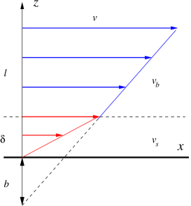
Figure 2: Slip length $b$ for a binary mixture.

Indeed, in a sharp interface limit, when the width of the interface is much smaller than the width of the slab and the thickness of the boundary layer, we can neglect the structure of the interface. Then the problem is reduced to the shear flow of two phases ($s$ for “surface”, $b$ for “bulk”) with viscosities $\eta_{s}$ and $\eta_{b}$, respectively, and thicknesses $\delta$ and $l$, respectively (see Fig. 2). Denoting the velocity profiles in the surface layer and the bulk by $v_{s}(z)$ and $v_{b}(z)$, respectively, and using stick boundary conditions at $z=0$ and $z=l+\delta$, we have

$$v_{s}(0) = 0,$$

$$v_{s}(\delta) = v_{b}(\delta),$$ (2)

$$v_{b}(l+\delta) = v_{0},$$

where the second equation is the condition for continuity of the flow field at the interface between the phases, and $v_{0}$ is the velocity at the top of the slab. Furthermore, we use the condition of zero divergence of the shear stress tensor at the interface,

$$\partial_{z}\left(\eta(z)\partial_{z}v(z)\right)=0,$$ (3)

or

$$\eta_{s}v^{\prime}_{s}(\delta)=\eta_{b}v^{\prime}_{b}(\delta).$$ (4)

The solution in the bulk

$$v_{b}(z)=\kappa v_{0}\left(\frac{\eta_{b}}{\eta_{s}}-1+\frac{z}{\delta}\right),$$ (5)

with $\kappa=\left({\eta_{b}}/{\eta_{s}}+{l}/{\delta}\right)^{-1}$, results in a slip length vinogradova.oi:1995.b

$$b=\delta\left(\frac{\eta_{b}}{\eta_{s}}-1\right).$$ (6)

According to Eq. (6) the boundary slip can be observed if the viscosity depends on the composition ($\eta_{b}\neq\eta_{s}$) and the less viscous fraction of the liquid wets the walls better than the more viscous one ($\eta_{b}>\eta_{s}$). It is also clear that there are two ways to obtain a large slip length. First, by having a macroscopically thick boundary layer, since the slip length has the same order of magnitude as the thickness of this layer. Second, by providing large values of the viscosity contrast $\eta_{b}/\eta_{s}$, e.g. for a gas layer .

A more realistic description should allow for a prewetting transition binder.k:1983.a ; bonn.d:2001.a for the liquid/gas or liquid/lubricant mixture and take into account the structure and the finite width of the interface region.

The aim of this paper is to include these effects and relate the slip length to the wettability of the walls, composition of the mixture, and thermodynamic parameters of the system. We show that the prewetting transition can give rise to a large boundary slip of the fluid by generating a thick film of a phase-separated ‘lubricant’ at the wall which has a lower than the bulk fluid viscosity. Indeed, if we choose typical values, thickness of the wetting layer (thick film) $\delta\approx 10\rm nm$, viscosity contrast $\eta_{b}~{}:~{}\eta_{s}=3~{}:~{}1$, we find $b\approx 20\rm nm$, i.e. the prewetting film can indeed give a large slip length. This value can be further increased. Indeed, if the phase separation occurs upon cooling (heating), the thickness of the wetting layer increases with the increase (decrease) of the temperature: for a system with short-range forces in the vicinity of the wetting temperature $T_{w}$, the thickness diverges as bonn.d:2001.a $\delta\propto-\ln\left(\left|T_{w}-T\right|\right)$.

The paper is organized as follows. In Sec. II we outline the approach that allows us to calculate the phase diagram, order parameter profiles, and slip length. Section III gives a summary of the results. Finally, in Sec. IV, we present some brief conclusions.

II Theoretical Model

Phase separation phenomena in binary and polymer mixtures have been intensively studied by theory, experiment, and simulation. While the most detailed information is available for the static bulk behavior, much more interesting phenomena occur when studying the dynamics gunton.jd:1983.a ; bray.aj:1994.a ; wagner.aj:1998.a ; kendon.vm:1999.a , or the behavior near surfaces and in confined geometries binder.k:1983.a ; dietrich.s:1988.a ; binder.k:2003.a ; duenweg.b:2003.a . The theoretical understanding of phenomena which combine both aspects (i. e. dynamics near surfaces) is still at its infancy puri.s:1994.a , while there are many experiments tanaka.h:1993.a ; tanaka.h.1993.c ; vinogradova.oi:1995.b .

Our theoretical approach splits the problem of shear flow of a binary mixture near surfaces into several independent tasks. First, we calculate the equilibrium order parameter profiles, completely disregarding the flow. Restriction to equilibrium thermodynamics allows us to introduce a change of ensemble: we fix the chemical potential difference (semi-grand-canonical ensemble) instead of fixing the composition, which is conceptually and computationally easier. The order parameter profile then results in a viscosity profile, which in turn allows us to calculate the stationary velocity profile by solving Eq. (3), again using stick boundary conditions at both surfaces. It is not immediately obvious that this split–up is justified. We discuss the restrictions and underlying assumptions of this approach in Appendix A. Finally, the slip length is calculated from the stationary velocity profile.

II.1 Free Energy of a Binary Mixture

To describe the bulk phase as well as the interface structure, ‘phase-field’ models binder.k:1983.a are often used. In this approach the order parameter $\phi$ is introduced. For a binary mixture $\phi$ is a composition variable, defined as $\phi=(n_{1}-n_{2})/(n_{1}+n_{2})$, where the $n_{i}$ are the number densities of the two species. This order parameter varies slowly in the bulk regions and rapidly on length scales of the interfacial width. The unmixing thermodynamics is described via a free energy functional.

Since the material is confined in a container in any experiment, phase separation is always affected by surface effects evans.r:1986.a ; evans.r:1987.a ; gelb.ld:1997.a ; gelb.ld:1997.b ; gelb.ld:1999.a . To include them, appropriate surface terms responsible for the interaction of the liquid with the container walls are added to the free energy cahn.jw:1977.a ; binder.k:1983.a ; degennes.pg:1985.a ; dietrich.s:1988.a ; bonn.d:2001.a ; schick.m:1990.a .

In the phase-field approach the semi-grand potential of a binary mixture is written as bonn.d:2001.a

$${\Omega}\{\phi\}=\frac{1}{a^{3}}\int dV\left[\frac{k}{2}a^{2}\left(\nabla\phi\right)^{2}+f(\phi)-\mu\phi\right]+\Psi_{s},$$ (7)

where $a$ is a normalization length of the order of the size of a molecule, $f(\phi)$ is the Helmholtz free energy density of the mixture, while $\mu$ is the chemical potential thermodynamically conjugate to the order parameter $\phi$, and $\Psi_{s}$ is the surface energy.

The explicit form of the Helmholtz free energy $f(\phi)$ varies depending on the type of mixture. However, the simple observation that the two phases must coexist implies that there are two minima in the free energy at the respective values of the order parameter. We here adopt the mean-field model for a regular (symmetric) mixture reichl.le:1998.a ; rowlinson.js:1969.a

$$f(\phi) = \frac{\chi}{4}(1-\phi^{2})+$$ (8)

$$k_{B}T\left[\frac{1+\phi}{2}\ln\frac{1+\phi}{2}+\frac{1-\phi}{2}\ln\frac{1-\phi}{2}\right],$$

where the first term on the right-hand side corresponds to the excess energy of mixing. Note that this is one of the simplest models to describe unmixing; a more realistic description would need a more sophisticated function, which also takes into account a dependence on the overall density, which can vary along the profile (see Appendix A).

The term $\left(\nabla\phi\right)^{2}$ is needed to provide spatial structure to the theory: at phase coexistence, there are two bulk equilibrium order parameter values $\phi_{+}$ and $\phi_{-}$ with the same free energy density, $f(\phi_{+})=f(\phi_{-})$. Without the gradient term, a structure with very many interfaces between the $\phi_{+}$ and $\phi_{-}$ phase would be entropically favored. The term $(k/2)\left(\nabla\phi\right)^{2}$ is the simplest one which penalizes interfaces. While this is justified near the critical point, where interfaces are very wide and the order parameter varies smoothly, a more realistic description at strong segregation (where the interface becomes rather sharp) would require higher–order gradients, too.

II.2 Surface Free Energy

To describe the interaction with the walls we used the quadratic approximation for the surface energy bonn.d:2001.a ; flebbe.t:1996.a

$$\Psi_{s}=\frac{1}{a^{2}}\int\left[-h\phi_{s}-\frac{1}{2}\gamma\phi_{s}^{2}\right]dS,$$ (9)

where $\phi_{s}$ is the surface value of the order parameter and the parameters $h$ and $\gamma$ are referred to as the short-range surface field and the surface enhancement, respectively. The short-range surface field, $h$, is a measure of the attractiveness (or repulsiveness, if negative) of the surface to the component $1$. In real systems it can be of either sign and of any magnitude. The surface coupling enhancement, $\gamma$, represents the effect that a molecule close to the substrate has fewer neighbors than a molecule in the bulk; $\gamma$ is estimated to be small and negative. We have implicitly assumed that all surface effects are of short range, thus $f_{s}$ depends on the local concentration at the walls only. Because of long range van der Waals forces this is not fully realistic. However, for large enough wall separations the differences to the short range case are rather minor.

We introduce dimensionless units by setting $a=1$, $\chi=1$, and $k_{B}=1$. Hence, energies are given in units of $\chi$, temperatures in units of $\chi/k_{B}$, and lengths in units of $a$. Furthermore, a value of $k=1$ has been used throughout the calculations of this paper.

II.3 Euler-Lagrange Equations

In thermal equilibrium the grand potential (7) must be minimal. Variation of this functional yields an Euler-Lagrange equation together with two boundary conditions. Due to translational symmetry in $x$ and $y$ direction, the problem is one-dimensional. In contrast to the situation considered in Introduction, we now focus on the case of two identical walls separated by a distance $L$, which is chosen large enough such that the two wetting layers do not overlap, and bulk behavior is established in the center of the slab. It is then convenient to choose the origin of the coordinate system at the center of the film. In this coordinate system the Euler-Lagrange equation and boundary conditions read

$$k\frac{\partial^{2}\phi}{\partial z^{2}}+\frac{1}{2}\phi-\frac{1}{2}T\ln\frac{1+\phi}{1-\phi}+\mu=0,$$ (10)

$$\pm k\left.\frac{\partial\phi}{\partial z}+h+\gamma\phi\right|_{z=-L/2,L/2}=0.$$ (11)

This boundary-value problem was solved using the relaxation method press.wh:1992.a . In general, it can have up to three different solutions: one stable, one metastable, and one unstable. The relaxation method yields only the metastable and the stable solution. The unstable solution with the highest free energy has negative response function $(\partial\phi/\partial\mu)_{T}$ and is eliminated by the relaxation method automatically.

To select stable solutions, we calculated the grand potential of the mixture, $\Omega$, for both stable and metastable solutions and chose the solution with the lowest grand potential. This allows the accurate determination of the phase diagram.

II.4 Velocity Profiles and Slip Length

To calculate the velocity profiles, we assumed that the viscosity of the system is simply a linear combination of that of the individual components

$$\eta(z)=\eta_{s}\frac{1+\phi(z)}{2}+\eta_{b}\frac{1-\phi(z)}{2},$$ (12)

where the viscosity contrast between the two components has been chosen as $\eta_{s}:\eta_{b}=1:3$. Of course, a more realistic description would have to introduce a more complicated dependence on $\phi$, and also take into account the dependence on the overall density. The stationary velocity profile is the solution of Eq. (4)

$$v(z)=v_{\rm w}c^{-1}\int_{-L/2}^{z}\frac{dz}{\eta(z)},$$ (13)

where

$$c=\int_{-L/2}^{L/2}\frac{dz}{\eta(z)},$$ (14)

and we assumed stick boundary conditions at the walls, $v(-L/2)=0$ and $v(+L/2)=v_{\rm w}$. The value of the slip length was obtained by fitting the bulk region of the velocity profile (13) with a linear regression.

III Results and Discussion

III.1 Order Parameter Profiles and Prewetting Phase Diagram

Typical order parameter profiles at the same value of the chemical potential $\mu=-0.002$ and a set of temperatures are shown in Fig. 3. Only the profiles corresponding to the stable thermodynamic state are shown. The profiles have a well-developed flat region in the center of the film, which indicates that there should not be finite size effects for the chosen thickness of the slab ($L=200$). This flat region is important for defining the slip length, see Eq. (1). This requires a well-defined linear velocity profile in the bulk.

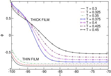
Figure 3: Typical order parameter profiles. Only the part next to the wall is shown. Thickness of the slab $L=200$, $\mu=-0.002$, $\gamma=-0.01$, $h=0.2$. For this chemical potential the thin-thick film transition occurs at $T\approx 0.35$.

In order to understand these profiles, one should note that the very small value of $\mu$, combined with the low temperature, implies that the system is rather close to bulk coexistence. Bulk coexistence, however, is characterized by two equilibrium values of the order parameter with large absolute value and opposite sign. The small negative value of $\mu$ singles out the negative order parameter value, while the absolute value is only slightly changed. Introducing the surface with preference of the other phase, one obtains a profile which is slightly bent up near the surface. The prewetting transition (see Refs. cahn.jw:1977.a ; schick.m:1990.a ) occurs upon increasing the temperature, and results in a sudden increase of the surface excess coverage, i. e. it is a first-order transition between a thin-film and a thick-film state. This jump is directly observed at a temperature near $T=0.35$ in the profiles of Fig. 3. Taking into account the remarks made in the introduction and Eq. (6), we can already anticipate small slip lengths for thin films and large slip lengths for thick films (above the prewetting transition temperature). Since the thin-thick film transition is a first-order transition, one can also expect a jump in the slip length at the prewetting transition temperature.

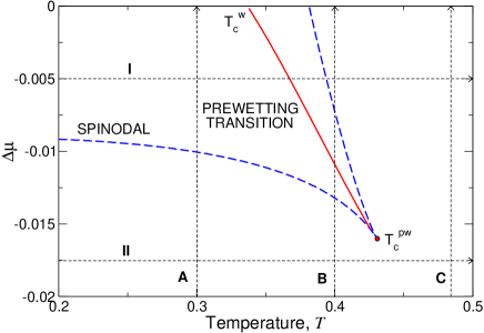
Figure 4: Prewetting phase diagram calculated for $h=0.2$, $\gamma=-0.01$, $L=200$. The solid line is the prewetting transition line ending at the prewetting critical point. Metastability limits of thick and thin films (spinodals) are shown with dashed lines. $\rm A$, $\rm B$, $\rm C$, $\rm I$, and $\rm II$ are thermodynamic paths used in the text.

To calculate the thin-thick film transition temperature, we followed the metastable solution up to its stability limit (spinodal) calculating the grand potential for both stable and metastable solutions. The transition line was determined from the intersection of grand potentials of stable and metastable solutions (thick and thin films). Both spinodals as well as the transition line are shown in a prewetting transition phase diagram, Fig. 4. The solid curve is the prewetting curve ending at the prewetting critical point and the dashed curves are spinodals or metastability limits of the metastable states.

III.2 Slip Length

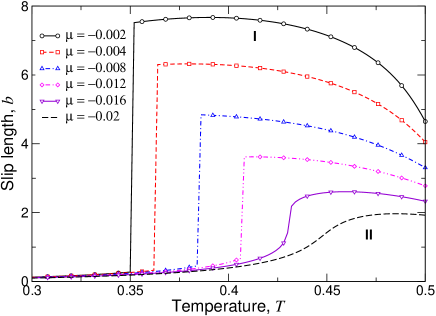
Figure 5: Slip length vs. temperature calculated for several values of the chemical potential. $h=0.2$, $\gamma=-0.01$, $L=200$.

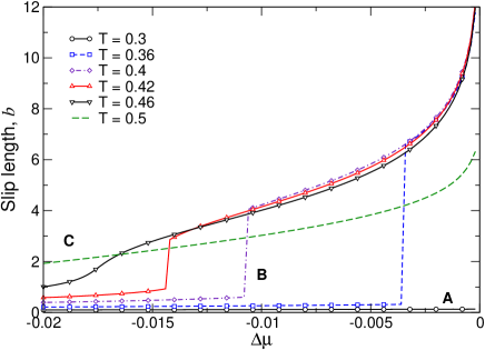
Figure 6: Slip length vs. chemical potential difference. $h=0.2$, $\gamma=-0.01$, $L=200$.

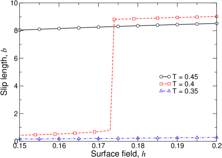
Figure 7: Slip length vs. short-range surface field. $\mu=-0.001$.

The temperature dependence of the slip length for several values of the chemical potential (or average volume fraction) is presented in Fig. 5. As we anticipated, $b(T)$ has a jump at the prewetting transition temperature, when the thick film is formed (path $\rm I$ in Fig. 4). Before the jump the slip length is small and practically does not depend on temperature. After the transition the slip length decreases with the temperature increasing, even though the prewetting film gets thicker. This is because the bulk volume fraction (order parameter $\phi$) increases, giving rise to a decrease in the bulk viscosity (or, equivalently, viscosity contrast) (see Fig. 3).

If we are above the prewetting critical point (path $\rm II$ in Fig. 4) there is no jump-like transition, but rather a smooth increase of the slip length with the temperature.

The dependence of the slip length on the chemical potential is shown in Fig. 6. If the temperature is below $T_{\rm c}^{\rm w}$ then the thin film is always stable and the slip length is small (path A in Fig. 4). Once we intersect the prewetting transition line, the thick film forms with the increase of the average fraction of the more wettable phase (values of the chemical potential close to zero) and the slip length jumps abruptly to higher values (path B in Fig. 4). Above the prewetting critical point $T_{\rm c}^{\rm pw}$ the slip length increases monotonically with the increase of the chemical potential (see path $\rm C$ in Fig. 4).

Finally, the dependence of the slip length on the surface field $h$ is shown in Fig. 7. It is clear that there is a threshold value of the surface field (contact angle) when the thick film is formed. At this value of the surface field the slip length increases abruptly. Below the threshold the slip length is small and practically does not depend on the surface field.

IV Conclusions

To summarize, when the prewetting transition occurs in a flow experiment, it may indeed generate a strong slippage. Prewetting provides a mechanism of generating a macroscopically thick film at the wall. If this film has a lower viscosity than the bulk value, a strong slippage can be observed above the prewetting transition temperature. The value of the slip length has a jump-like dependence on temperature, concentration of the phase-separated liquid, and surface field (contact angle).

The mean-field model of wetting is rather general and can be applied to liquid-gas systems, binary mixtures, as well as incompressible polymer mixtures in the long wavelength approximation flebbe.t:1996.a . This implies that the large boundary slip due to prewetting can be observed in all these systems.

Another goal of this paper is to stimulate accurate quantitative measurements of the slip length combined with measurements of the fluid wetting properties. This will allow to study the underlying microscopic mechanisms of slippage, and choose an adequate model for every experimental situation. In particular, it would be very interesting to measure the slip length as a function of temperature while the system undergoes a prewetting transition, with the adsorbed species having a lower viscosity. Our results indicate that in such a case the slip length should undergo an abrupt change, and we believe that this will be true beyond the limitations of our idealized model.

Appendix A Hydrodynamics of Slippage in Binary Fluids

We consider a binary fluid (species $1$ and $2$) confined between two infinite parallel planes to a thin slab of thickness $L$. The plane normal is in the $z$ direction. We denote the mass densities of the two species by $\rho_{1}$ and $\rho_{2}$, respectively, and introduce the linear combinations $\rho=\rho_{1}+\rho_{2}$ (total mass density) and $\Delta\rho=\rho_{1}-\rho_{2}$.

Concerning the thermodynamics of the system, we notice that the pressure tensor $p_{\alpha\beta}$ (Greek letters denote Cartesian indices) is anisotropic as a result of the finite size effect and the interface contribution to the free energy allen.mp:2000.a . Since the system is fluid, there is no elastic response to shear, and hence $p_{\alpha\beta}=0$ for $\alpha\neq\beta$. Furthermore, $p_{xx}=p_{yy}$ for symmetry reasons. Apart from this anisotropy, we assume that there is no further inherent anisotropy. In particular, we assume that all transport coefficients (interdiffusion coefficient, thermodiffusion coefficient, viscosities, etc.) retain their simple scalar nature as in the isotropic macroscopic bulk fluid. The viscous stress tensor is hence written as

$$\sigma_{\alpha\beta}=\eta\left(\partial_{\alpha}v_{\beta}+\partial_{\beta}v_{\alpha}-\frac{2}{3}\delta_{\alpha\beta}\partial_{\gamma}v_{\gamma}\right)+\zeta\delta_{\alpha\beta}\partial_{\gamma}v_{\gamma},$$ (15)

where the Einstein summation convention is implied, $\bm{v}$ denotes the fluid flow velocity, while $\eta$ and $\zeta$ are the shear and the bulk viscosity, respectively. We assume that these parameters depend on density and composition, i. e. $\eta=\eta(\rho,\Delta\rho)$ and $\zeta=\zeta(\rho,\Delta\rho)$.

We consider the situation that the fluid is weakly driven such that a shear flow in $x$ direction develops, with shear gradient in $z$ direction. In this limit of weak driving, it is reasonable to assume that no symmetry is broken except translational invariance in $z$ direction. The system remains translationally invariant in $x$ and $y$ direction, and gradients (of any quantity) occur only in $z$ direction. We also assume that the system is kept at constant temperature throughout, i. e. that the heat production is negligibly small. This is reasonable for small shear rates (note that the heat production is proportional to the square of the shear rate). In addition, the heat conductivity is quite large for many real fluids.

Under these assumptions, we seek a stationary solution of the hydrodynamic equations of motion landau.ld:1995.a for the outlined geometry and symmetry. Since the velocity flow field $\bm{v}=(v_{x},0,0)$ is defined as the center–of–mass velocity of a volume element, the dynamics of $\rho$ is governed by pure convection:

$$\partial_{t}\rho+\partial_{\alpha}\left(\rho v_{\alpha}\right)=0.$$ (16)

A stationary solution implies $\partial_{t}\rho=0$, while our geometry leads to $\partial_{\alpha}\left(\rho v_{\alpha}\right)=\partial_{z}\left(\rho(z)v_{z}\right)=0$. The continuity equation is therefore identically fulfilled, and a non–constant mass density profile $\rho(z)$ is permitted.

For the density difference there is also interdiffusion:

$$\partial_{t}\Delta\rho+\partial_{\alpha}\left(\Delta\rho v_{\alpha}\right)=-\partial_{\alpha}j_{\alpha},$$ (17)

where $\bm{j}$ is the interdiffusion current. Again, the left hand side vanishes identically for our flow. Furthermore, the interdiffusion current vanishes in the stationary state:

$$\bm{j}=0.$$ (18)

The (full nonlinear) Navier–Stokes equation is written as

$$\partial_{t}\left(\rho v_{\alpha}\right)+\partial_{\beta}\left(\rho v_{\alpha}v_{\beta}\right)=-\partial_{\beta}p_{\alpha\beta}+\partial_{\beta}\sigma_{\alpha\beta}.$$ (19)

For our flow, the left hand side vanishes identically, and hence

$$\partial_{z}p_{zz} = \partial_{z}\sigma_{zz}=0,$$ (20)

$$0=\partial_{z}p_{xz}(z) = \partial_{z}\sigma_{xz}=\partial_{z}\left(\eta\partial_{z}v_{x}\right),$$ (21)

$$0=\partial_{z}p_{yz} = \partial_{z}\sigma_{yz}=0.$$ (22)

From Eq. (20) one sees that the pressure profile $p_{zz}$ must be constant, while Eq. (21) allows to obtain the velocity profile via integration, as soon as the viscosity profile $\eta(z)$ is known from the profiles $\rho(z)$ and $\Delta\rho(z)$.

We now turn to the constitutive equation for the interdiffusion current $\bm{j}$. In non–equilibrium thermodynamics, the dissipative currents are assumed to be linear in the gradients of the intensive thermodynamic variables. A binary system has three independent thermodynamic variables, for which we can take any appropriate set. For our purposes it is particularly useful to choose the pressure $p$, the temperature $T$, and the chemical potential $\mu$, which is defined as the variable which is thermodynamically conjugate to the order parameter $\phi=(n_{1}-n_{2})/(n_{1}+n_{2})$, where the $n_{i}$ denote the particle number densities (see main text). Macroscopically, the constitutive equation would thus read

$$j_{\alpha}=-\Gamma_{1}\partial_{\alpha}\mu-\Gamma_{2}\partial_{\alpha}T-\Gamma_{3}\partial_{\alpha}p,$$ (23)

where $\Gamma_{i}$ are suitable scalar Onsager coefficients. Note that the pressure gradient may appear since $\mu$ is not the variable conjugate to $\Delta\rho/\rho$ (which is often used in the literature landau.ld:1995.a ), but rather to $\phi$. We now generalize this equation to the case of an anisotropic pressure tensor, but retain the scalar nature of the Onsager coefficients in accordance with our assumptions (similar to what is done in model H kendon.vm:2001.a ; zhang.zh:2001.a ). We thus find

$$j_{\alpha}=-\Gamma_{1}\partial_{\alpha}\mu-\Gamma_{2}\partial_{\alpha}T-\Gamma_{3}\partial_{\beta}p_{\alpha\beta},$$ (24)

or, taking into account that there are only gradients in $z$ direction, and that $\bm{j}$ vanishes,

$$0=-\Gamma_{1}\partial_{z}\mu-\Gamma_{2}\partial_{z}T-\Gamma_{3}\partial_{z}p_{zz}.$$ (25)

Now, $\partial_{z}T$ vanishes due to our assumption of an isothermal system, while $\partial_{z}p_{zz}$ vanishes as a consequence of the Navier–Stokes equation (see Eq. 20). For this reason, the profile of the chemical potential, $\mu(z)$, must be a constant, too.

In summary, we find that under the given assumptions (isothermal system, isotropic Onsager coefficients, weak driving) the conditions for the stationary state are identical to those in thermal equilibrium (all intensive variables must have constant profiles). This permits to first calculate the density profiles just as equilibrium profiles, completely disregarding the flow, and then, in a second step, to calculate the velocity profile by solving Eq. (21). This has been done in the main text for a simple model for the unmixing thermodynamics, and a linear dependence of the viscosity $\eta$ on the order parameter. Note also that the restriction to pure equilibrium thermodynamics allows us to introduce a change of ensemble: instead of considering the composition as fixed, we rather view $\mu$ as fixed (semi–grand ensemble), which is conceptually and computationally easier. Of course, a quantitative comparison with experiments is not possible for such simple models; one would have to use much more sophisticated free energy functionals, and a better model for the concentration dependence of $\eta$ as well. Furthermore, one should expect that at moderate shear rates only hydrodynamic instabilities (e. g. bubble formation near the surfaces) should occur which invalidate the assumption of translational invariance in $x$ and $y$ direction.

- (1) G. K. Batchelor, An Introduction to Fluid Dynamics (Cambridge University Press, Cambridge, 2000).
- (2) O. I. Vinogradova, Int. J. Miner. Process. 56, 31 (1999).
- (3) N. V. Churaev, V. D. Sobolev, and A. N. Somov, J. Colloid Interface Sci. 97, 574 (1984).
- (4) K. Watanabe, Y. Udagawa, and H. Udagawa, J. Fluid Mech. 381, 225 (1999).
- (5) R. Pit, H. Hervet, and L. Leger, Phys. Rev. Lett. 85, 980 (2000).
- (6) D. C. Tretheway and C. D. Meinhart, Phys. Fluids 14, L9 (2002).
- (7) D. Lumma, A. Best, A. Gansen, F. Feuillebois, J. O. Rädler, and O. I. Vinogradova, Phys. Rev. E 67, 056313 (2003).
- (8) J. Krim, Sci. Am. 275, 48 (1996).
- (9) R. G. Horn, O. I. Vinogradova, M. E. Mackay, and N. Phan-Thien, J. Chem. Phys. 112, 6424 (2000).
- (10) Y. X. Zhu and S. Granick, Phys. Rev. Lett. 87, 096105 (2001).
- (11) Y. X. Zhu and S. Granick, Phys. Rev. Lett. 88, 106102 (2002).
- (12) J. Baudry, E. Charlaix, A. Tonck, and D. Mazuyer, Langmuir 17, 5232 (2001).
- (13) V. S. J. Craig, C. Neto, and D. R. M. Williams, Phys. Rev. Lett. 87, 054504 (2001).
- (14) O. I. Vinogradova and G. E. Yakubov, Langmuir 19, 1227 (2003).
- (15) F. Brochard and P. G. de Gennes, Langmuir 8, 3033 (1992).
- (16) A. Ajdari, F. Brochard-Wyart, P. G. de Gennes, L. Leibler, J. L. Viovy, and M. Rubinstein, Physica A 204, 17 (1994).
- (17) F. Brochard-Wyart, C. Gay, and P. G. deGennes, Macromolecules 29, 377 (1996).
- (18) O. Francescangeli, F. Simoni, S. Slussarenko, D. Andrienko, V. Reshetnyak, and Y. Reznikov, Phys. Rev. Lett. 82, 1855 (1999).
- (19) M. Sun and C. Ebner, Phys. Rev. A 46, 4813 (1992a).
- (20) M. Sun and C. Ebner, Phys. Rev. Lett. 69, 3491 (1992b).
- (21) L. Bocquet and J.-L. Barrat, Phys. Rev. Lett. 70, 2726 (1993).
- (22) P. A. Thompson and S. M. Troian, Nature 389, 360 (1997).
- (23) J. L. Barrat and L. Bocquet, Faraday Discuss. 112, 119 (1999a).
- (24) J. L. Barrat and L. Bocquet, Phys. Rev. Lett. 82, 4671 (1999b).
- (25) M. Cieplak, J. Koplik, and J. R. Banavar, Phys. Rev. Lett. 86, 803 (2001).
- (26) V. P. Sokhan, D. Nicholson, and N. Quirke, J. Chem. Phys. 115, 3878 (2001).
- (27) C. Cottin-Bizonne, J. L. Barrat, L. Bocquet, and E. Charlaix, Nat. Mater. 2, 237 (2003).
- (28) L. M. Hocking, J. Fluid Mech. 76, 801 (1976).
- (29) I. V. Ponomarev and A. E. Meyerovich, Phys. Rev. E 67, 026302 (2003).
- (30) E. Ruckenstein and P. Rajora, J. Colloid Interface Sci. 96(2), 488 (1983).
- (31) P. G. de Gennes, Langmuir 18, 3413 (2002).
- (32) O. I. Vinogradova, N. F. Bunkin, N. V. Churaev, O. A. Kiseleva, A. V. Lobeyev, and B. W. Ninham, J. Colloid Interface Sci. 173, 443 (1995).
- (33) H. Tanaka, J. Phys.-Condens. Matter 13, 4637 (2001).
- (34) H. Tanaka, Phys. Rev. Lett. 70, 53 (1993a).
- (35) O. I. Vinogradova, Langmuir 11, 2213 (1995).
- (36) K. Binder, in Phase Transitions and Critical Phenomena, edited by C. Domb and J. Lebowitz (Academic Press, 1983), vol. 8, pp. 2–144.
- (37) D. Bonn and D. Ross, Rep. Prog. Phys. 64, 1085 (2001).
- (38) J. D. Gunton, M. S. Miguel, and P. S. Sahni, in Phase Transitions and Critical Phenomena, edited by C. Domb and J. Lebowitz (Academic Press, 1983), vol. 8, p. 269.
- (39) A. J. Bray, Adv. Phys. 43, 357 (1994).
- (40) A. J. Wagner and J. M. Yeomans, Phys. Rev. Lett. 80, 1429 (1998).
- (41) V. M. Kendon, J. C. Desplat, P. Bladon, and M. E. Cates, Phys. Rev. Lett. 83, 576 (1999).
- (42) S. Dietrich, in Phase Transitions and Critical Phenomena, edited by C. Domb and J. Lebowitz (Academic Press, 1988), vol. 12, p. 1.
- (43) K. Binder, D. P. Landau, and M. Müller, J. Stat. Phys. 110, 1411 (2003).
- (44) B. Dünweg, D. P. Landau, and A. I. Milchev, eds., Computer simulations of surfaces and interfaces (Kluwer, Dordrecht, 2003, to appear).
- (45) S. Puri and K. Binder, Phys. Rev. E 49, 5359 (1994).
- (46) H. Tanaka, Phys. Rev. Lett. 70, 3524 (1993b).
- (47) R. Evans, U. M. B. Marconi, and P. Tarazona, J. Chem. Phys. 84, 2376 (1986).
- (48) R. Evans and U. M. B. Marconi, J. Chem. Phys. 86, 7138 (1987).
- (49) L. D. Gelb and K. E. Gubbins, Phys. Rev. E 55, R1290 (1997a).
- (50) L. D. Gelb and K. E. Gubbins, Phys. Rev. E 56, 3185 (1997b).
- (51) L. D. Gelb, K. E. Gubbins, R. Radhakrishnan, and M. Sliwinskabartkowiak, Rep. Prog. Phys. 62, 1573 (1999).
- (52) J. W. Cahn, J. Chem. Phys. 66, 3667 (1977).
- (53) P. G. de Gennes, Rev. Mod. Phys. 57, 827 (1985).
- (54) M. Schick, in Les Houches Session XLVIII, 1988, edited by J. Charvolin (Amsterdam, Elsevier, 1990), p. 415.
- (55) L. E. Reichl, A modern course in statistical physics (John Wiley & Sons, New York, 1998).
- (56) J. S. Rowlinson, Liquids and liquid mixtures (Butterworth, London, 1969), 2nd ed.
- (57) T. Flebbe, B. Dünweg, and K. Binder, J. Phys. II 6, 667 (1996).
- (58) W. H. Press, B. P. Flannery, S. A. Teukolsky, and W. T. Vetterling, Numerical Recipes in Fortran (Cambridge University Press, Cambridge, 1992), 2nd ed.
- (59) M. P. Allen, Chem. Phys. Lett. 331, 513 (2000).
- (60) L. D. Landau and E. M. Lifshitz, Fluid Mechanics, vol. 6 of Course of Theoretical Physics (Butterworth-Heinemann, Oxford, 1995).
- (61) V. M. Kendon, M. E. Cates, I. Pagonabarraga, J. C. Desplat, and P. Bladon, J. Fluid Mech. 440, 147 (2001).
- (62) Z. Zhang, H. Zhang, and Y. Yang, J. Chem. Phys. 115, 7783 (2001).