Spectra of complex networks

Abstract

We propose a general approach to the description of spectra of complex networks. For the spectra of networks with uncorrelated vertices (and a local tree-like structure), exact equations are derived. These equations are generalized to the case of networks with correlations between neighboring vertices. The tail of the density of eigenvalues $\rho\left(\lambda\right)$ at large $\left|\lambda\right|$ is related to the behavior of the vertex degree distribution $P\left(k\right)$ at large $k$. In particular, as $P\left(k\right)\sim k^{-\gamma}$, $\rho\left(\lambda\right)\sim\left|\lambda\right|^{1-2\gamma}$. We propose a simple approximation, which enables us to calculate spectra of various graphs analytically. We analyse spectra of various complex networks and discuss the role of vertices of low degree. We show that spectra of locally tree-like random graphs may serve as a starting point in the analysis of spectral properties of real-world networks, e.g., of the Internet.

I Introduction

Many real-world technological, social and biological complex systems have a network structure. Due to their importance and influence on our life (recall, e.g., the Internet, the WWW, and genetic networks) investigations of properties of complex networks are attracting much attention [1, 2, 3, 4, 5, 6, 7]. Such properties as robustness against random damages and absence of the epidemic threshold in the so called “scale-free” networks are nontrivial consequences of their topological structure. Despite undoubted advances in uncovering the main important mechanisms, shaping the topology of complex networks, we are still far from complete understanding of all peculiarities of their topological structure. That is why it is so important to look for new approaches which can help us to reveal this structure.

The structure of networks may be completely described by the associated adjacency matrices. The adjacency matrices of undirected graphs are symmetric matrices with matrix elements, equal to number of edges between the given vertices. The eigenvalues of an adjacency matrix are related to many basic topological invariants of networks such as, for example, the diameter of a network [8, 9]. Recently, in order to characterize networks, it was proposed to study spectra of eigenvalues of the adjacency matrices as a fingerprint of the networks [10, 11, 12, 13, 14, 15, 16, 17]. The rich information about the topological structure and diffusion processes can be extracted from the spectral analysis of the networks. Studies of spectral properties of the complex networks may also have a general theoretical interest. The random matrix theory has been successfully  used to model statistical properties of complex classical and quantum systems such as complex nucleus, disordered conductors, chaotic quantum systems (see, for example, reviews [18]), the glassy relaxation [19] and so on.

As the adjacency matrices are random, in the limit $N\longrightarrow\infty$ ($N$ is the total number of vertices), the density of eigenvalues could be expected to converge to the semicircular distribution in accordance with the Wigner theorem [20]. However, Rodgers and Bray have demonstrated that the density of eigenvalues of a sparse random matrix deviates from the Wigner semicircular distribution and has a tail at large eigenvalues [21], see also [22]. Recent numerical calculations of the spectral properties of small-world and scale-free networks [12, 13, 14], and the spectral analyses of the Internet [10, 11, 15, 16] have also revealed that the Wigner theorem does not hold. The spectra of the Internet [10, 11] and scale-free networks [13, 14] demonstrate an unusual power-law tail in the region of large eigenvalues. At the present time there is a fundamental lack in understanding of these anomalies. In order to carry out a complete spectral analysis of real networks it is necessary to take into account all features of these complex systems described by a degree distribution, degree correlations, the statistics of loops, etc. At this time there is no regular approach that allows one to handle this problem. Our paper fills this gap.

Our approach is valid for any network which has a local tree-like structure. In particular, these are uncorrelated random graphs with a given degree distribution [23, 24], and their straightforward generalizations [25] allowing pair correlations of the nearest neighbors. These graph ensembles have one common property: almost every finite connected subgraph of the infinite graph is a tree. The tree is a graph, which has no loops. A random Bethe lattice is an infinite random tree-like graph. All vertices on a Bathe lattice are statistically equivalent [26]. These features (the absence of loops and the statistical equivalence of vertices) are decisive for our approach. The advantage of Bethe lattices is that they frequently allow analytical solutions for a number of problems: random walks, spectral problems, etc.

Real-world networks, however, often contain numerous loops. In particular, this is reflected in a strong “clustering”, which means that the (relative) number of loops of length $3$ do not vanish even in very large networks. Nevertheless, we believe, that the study of graphs with a local tree-like structure may serve as a starting point in the description of more complex network architectures.

In the present paper we will derive exact equations which determine the spectra of infinite random uncorrelated and correlated random tree-like graphs. For this, we use a method of random walks. We propose a method of an approximate solution of the equations. We shall show that the spectra of adjacency matrices of random tree-like graphs have a tail at large eigenvalues. In the case of a scale-free degree distribution, the density of eigenvalues has a power-law behavior. We will compare spectra of random tree-like graphs and spectra of real complex networks. The role of weakly connected vertices will also be discussed.

II General approach

Let $\hat{A}=\left(a_{vw}\right)$ be the $N\times N$ symmetric adjacency matrix of an $N$-vertex Mayer’s graph $G$, $a_{vw}^{2}=a_{vw}$, $a_{vv}=0$ (the Mayer graph has either $0$ or $1$ edges between any pair of vertices, and has no “tadpoles”, i.e., edges attached at a single vertex). Degree $k_{v}$ (the number of connections) of a vertex $v$ is defined as

$$k_{v}=\sum_{w}a_{vw}\,.$$ (1)

A random graph, which is, in fact, an ensemble of graphs, is characterized by a degree distribution $P(k)$:

$$P\left(k\right)=\left\langle\frac{1}{N}\sum_{v=1}^{N}\delta\left(k_{v}-k\right)\right\rangle\,.$$ (2)

Here, $\langle\ \rangle$ is the averaging over the ensemble. We suppose that each graph in the ensemble has $N$ vertices. Graph ensembles with a given uncorrelated vertex degree distribution may be realized, e.g., as follows. Consider all possible graphs with a sequence of the numbers $\{N\left(k\right)\}$ of vertices of degree $k$, $k=1,2,\dots$, $\sum_{k}N(k)=N$, assuming $N\left(k\right)/N\to P\left(k\right)$ in the thermodynamic limit [$N(k)\to\infty$, $N\to\infty$]. Suppose that all these graphs are equiprobable. Then, simple statistical arguments lead to the conclusion that almost all finite connected subgraphs of an infinite graph do not contain loops.

This approach can be easily generalized to networks with correlations between nearest-neighbor vertices, characterized by the two-vertex degree distribution:

$$P_{2}\left(k,k^{\prime}\right)=\left\langle\frac{1}{2L}\sum_{v,w=1}^{N}a_{vw}\delta\left(k_{v}-k\right)\delta\left(k_{w}-k^{\prime}\right)\right\rangle\,.$$ (3)

Here $L=\left(1/2\right)\sum_{v,w}a_{vw}$ is the total number of edges. In the case of an uncorrelated graph we have

$$P_{2}\left(k,k^{\prime}\right)=\frac{kk^{\prime}}{{\langle k\rangle}^{2}}P\left(k\right)P\left(k^{\prime}\right)\,,$$ (4)

where $\langle k\rangle=2L/N$ is the mean degree of a vertex.

The spectrum of $\widehat{A}$ may be calculated by using the method of random walks on a tree-like graph $G$ and generating functions [27]. We define a generating function

$$R(z)=\frac{1}{N}\sum_{v=1}^{N}\sum_{n=0}^{\infty}\rho_{v}(n)z^{n}\,,$$ (5)

where $\rho_{v}(n)$ is the number of walks of length $n$ from $v$ to $v$, where $v$ is any vertex of $G$:

$$\rho_{v}(n)=(\widehat{A}^{n})_{v,v}\,.$$ (6)

In a tree-like graph the number of steps $n$ is an even number. In order to return to $v$ we must go back along all of the edges we have gone.

Let $q_{v}(n)$ be the number of walks of length $n$ starting at $v$ and ending at $v$ for the first time. We define

$$Q_{v}(z)=\sum_{n=0}^{\infty}q_{v}(n)z^{n}\,.$$ (7)

One can prove that

$$R(z)=\frac{1}{N}\sum_{v=1}^{N}\frac{1}{1-Q_{v}(z)}\,.$$ (8)

Let $d(w,v)=m\geqslant 1$ be the distance from $w$ to $v$ and $t_{w,v}^{(m)}(n)$ be the the number of paths of length $n$ starting at $w$ and ending at $v$ for the first time. We define

$$T_{wv}^{(m)}(z)=\sum_{n=0}^{\infty}t_{w,v}^{(m)}(n)z^{n}\,.$$ (9)

One can prove

$$Q_{v}(z) = z\sum_{w}T_{wv}^{(1)}(z)\,,$$ (10)

$$T_{wv}^{(m)}(z) = T_{wg_{1}}^{(1)}(z)T_{g_{1}g_{2}}^{(1)}(z)...T_{g_{m-1}v}^{(1)}(z)\,,$$ (11)

where $w\longrightarrow g_{1}\longrightarrow g_{2}\longrightarrow...g_{m-1}\longrightarrow v$ is the shortest path from $w$ to $v$. There is an important relationship:

$$T_{wv}^{(1)}(z) = z+z\sum_{g}T_{gv}^{(2)}(z)$$ (12)

$$= z+z\sum_{g}T_{gw}^{(1)}(z)T_{wv}^{(1)}(z)\,.$$ (13)

In this sum the vertex $g$ is the nearest neighbor of $w$ and a second neighbor of the vertex $v$. Solving the recurrence equation (13), we can find $T_{wv}^{(1)}(z)$ and $Q_{v}(z)$.

We define $\widetilde{T}_{wv}^{(1)}(z)\equiv T_{wv}^{(1)}(z^{-1})$. Equation (13) may be written in a form

$$\widetilde{T}_{wv}^{(1)}(z)=\frac{1}{z-\sum_{g}\widetilde{T}_{gw}^{(1)}(z)}\,.$$ (14)

We can find $Q_{v}(z)$, from which we get $R(z).$ Let us define $B(z)\equiv z^{-1}R(z^{-1})$. Then the density of the eigenvalues $\lambda$ of a random graph is determined as follows:

$$\rho(\lambda)=-\mathop{\rm Im}\left\langle B(\lambda+i\varepsilon))\right\rangle/\pi\,,$$ (15)

where $\varepsilon$ is positive and tends to zero. Note that the equations (7)–(14) are valid for both uncorrelated and correlated tree-like graphs.

In the case of a $k-$regular connected graph we have $\widetilde{T}_{wv}^{(1)}(z)\equiv T(z)$ and $Q_{v}(z)\equiv Q(z)$. Eq. (14) gives

$$zT(z)-(k-1)T^{2}(z)=1\,.$$ (16)

Solving this equation, we get the well known result:

$$\rho(\lambda)=\frac{k}{2\pi}\frac{\sqrt{4(k-1)-\lambda^{2}}}{k^{2}-\lambda^{2}}\,.$$ (17)

This is a continuous spectrum of extended eigenstates with eigenvalues $\left|\lambda\right|<2\sqrt{k-1}$. The presence of the denominator on the right-hand side of Eq. (17) leads to a difference of the spectrum of this graph from Wigner’s semi-circular law. In exact terms, Wigner’s law is valid for the eigenvalue spectra of real symmetric random matrices whose elements are independent identically distributed Gaussian variables [20]. These specific random matrices for Wigner’s law essentially differ from the adjacency matrices, which we consider in this paper. So, in our case, the semicircular law may be used only as a landmark for a contrasting comparison.

III Spectra of uncorrelated graphs

In the case of uncorrelated random tree-like graphs, $\ k_{w}-1$ random parameters $\widetilde{T}_{gw}^{(1)}(z)$ on the right-hand side of Eq. (14) are equivalent and statistically independent. They are also independent on the degree $k_{w}$. We define the distribution function of $\widetilde{T}_{wv}^{(1)}(z)$ at $z=\lambda+i\varepsilon$ in the Fourier representation as:

$$F_{\lambda}(x)=\left\langle\exp\left[-ix\widetilde{T}_{wv}^{(1)}(\lambda+i\varepsilon)\right]\right\rangle\,,$$ (18)

where the brackets $\left\langle...\right\rangle$ means the averaging over the ensemble of random uncorrelated graphs associated with a degree distribution $P(k)$. The statistical independence of the $k-1$ random parameters $\widetilde{T}_{gw}^{(1)}(\lambda+i\varepsilon)\equiv T_{i}$, $i=1,2,...k-1$, $k\equiv k_{w}$, on the right hand side of Eq. (14) allows us to use the following identity:

$$F_{\lambda}(x)\equiv\left\langle\exp(-ixT)\right\rangle=\left\langle\exp(-\frac{ix}{\lambda+i\varepsilon-\sum_{i=1}^{k-1}T_{i}})\right\rangle$$ (19)

$$= 1-\sqrt{x}\int\limits_{0}^{\infty}\frac{dy}{\sqrt{y}}J_{1}(2\sqrt{xy})\left\langle\exp(iy[\lambda+i\varepsilon-\sum_{i=1}^{k-1}T_{i}])\right\rangle$$ (20)

$$= 1-\sqrt{x}\int\limits_{0}^{\infty}\frac{dy}{\sqrt{y}}J_{1}(2\sqrt{xy})e^{iy(\lambda+i\varepsilon)}\times$$ (22)

$$\sum_{k}\frac{kP(k)}{\langle k\rangle}\left\langle\exp(-iyT)\right\rangle^{k-1}\,,$$

where $J_{1}(x)$ is the Bessel function and $\left\langle k\right\rangle=\sum_{k}kP(k)$. Thus, we get the exact self-consistent equation for $F_{\lambda}(x)$:

$$F_{\lambda}(x)=1-\sqrt{x}\int_{0}^{\infty}\frac{dy}{\sqrt{y}}J_{1}(2\sqrt{xy})e^{iy\lambda}\Phi_{1}(F_{\lambda}(y))\,,$$ (23)

where $\Phi_{1}(x)\equiv\sum_{k=1}^{\infty}kP(k)x^{k-1}/\left\langle k\right\rangle$. Solving Eq. (23) gives the distribution of $T$, and  so we can obtain $Q$, from which we get $R$. Eqs. (8), (10), and (15) give

$$\rho(\lambda) = -\frac{1}{\pi}\mathop{\rm Im}\left\langle\frac{1}{\lambda-\sum_{i=1}^{k}T_{i}}\right\rangle$$ (24)

$$= \frac{1}{\pi}\mathop{\rm Re}\int_{0}^{\infty}dye^{iy\lambda}\Phi(F_{\lambda}(y))\,,$$ (25)

where $\Phi(x)\equiv\sum_{k=1}^{\infty}P(k)x^{k}$. From Eq. (23), we find the $n$-th moment of the distribution function $\Psi_{\lambda}(T)$, Eq. (18):

$$M_{n}\equiv\left\langle T^{n}\right\rangle=\frac{1}{(n-1)!\,i^{n}}\int_{0}^{\infty}dy\,y^{n-1}e^{iy\lambda}\Phi_{1}(F_{\lambda}(y))\,.$$ (26)

IV Effective medium approximation

In a general case it is difficult to solve Eq. (23) exactly. Let us find an approximate solution. We neglect fluctuations of $T$ around a mean value $T(\lambda)\equiv\left\langle T\right\rangle$. A self-consistent equation for the function $T(\lambda)$ may be obtained if we insert

$$F_{\lambda}(x)\approx e^{-ixT(\lambda)}$$ (27)

into the right-hand side of Eq. (26) for $n=1$. We get

$$T(\lambda)=\frac{1}{\left\langle k\right\rangle}\sum_{k}\frac{kP(k)}{\lambda+i\varepsilon-(k-1)T(\lambda)}\,.$$ (28)

Below we will call this approach an “effective medium” (EM) approximation. At real $\lambda$, $T(\lambda)$ is a complex function, which is to be understood as an analytic continuation from the upper half-plane of $\lambda$, $T\left(\lambda\right)\equiv T\left(\lambda+i\varepsilon\right)$. Therefore, $\mathop{\rm Im}T(\lambda+i\varepsilon)<0$. In the framework of the EM approach, the density $\rho(\lambda)$, Eq. (25), takes an approximate form

$$\rho(\lambda)=-\frac{1}{\pi}\sum_{k}\frac{kP(k)\mathop{\rm Im}T(\lambda)}{(\lambda-k\mathop{\rm Re}T(\lambda))^{2}+k^{2}(\mathop{\rm Im}T(\lambda))^{2}}\,.$$ (29)

V Tail behavior and finite-size effect

Equation (28) may be solved analytically at $\left|\lambda\right|\gg 1$. We look for a solution in the region $\mathop{\rm Im}T(\lambda)\ll\mathop{\rm Re}T(\lambda)\ll 1$. It is convenient to use a continuum approximation in Eq. (28). The real and imaginary parts of this equation take a form

$$\mathop{\rm Re}T(\lambda)=\frac{1}{2\lambda\left\langle k\right\rangle}\times$$ (30)

$$\int_{k_{0}}^{k_{cut}}\!\!\!\!\!\!\!\!\frac{dk\,kP(k)}{\displaystyle\left(\!1-(k-1)\mathop{\rm Re}\frac{T(\lambda)}{\lambda}\right)^{\!2}\!+\left(\!(k-1)\mathop{\rm Im}\frac{T(\lambda)}{\lambda}\right)^{\!2}}\,,$$ (31)

$$1=\frac{1}{\lambda^{2}\left\langle k\right\rangle}\times$$ (32)

$$\int_{k_{0}}^{k_{cut}}\!\!\!\!\!\!\!\!\frac{dk\,k(k-1)P(k)}{\displaystyle\left(\!1-(k-1)\mathop{\rm Re}\frac{T(\lambda)}{\lambda}\right)^{\!2}\!+\left(\!(k-1)\mathop{\rm Im}\frac{T(\lambda)}{\lambda}\right)^{\!2}}\,,$$ (33)

where $k_{0}$ and $k_{cut}$ are the smallest and largest degrees, respectively. A region $k_{0}\leq k\ll k_{\lambda}$ gives a regular contribution into the integrals (31) and (33) while a region $k\sim k_{\lambda}\gg 1$ gives a singular contribution. Here $k_{\lambda}\equiv\lambda/\mathop{\rm Re}T(\lambda)+1$. As a result we obtain

$$\mathop{\rm Re} T(\lambda)\cong\frac{1}{2\lambda}+\frac{\pi k_{\lambda}P(k_{\lambda})}{2\left\langle k\right\rangle\mathop{\rm Im}T(\lambda)}\,,$$ (34)

$$1\cong\frac{1}{\lambda^{2}\left\langle k\right\rangle} \int_{k_{0}}^{k_{\lambda}}dk\,k(k-1)P(k)+\frac{\pi\lambda k_{\lambda}P(k_{\lambda})}{\left\langle k\right\rangle\mathop{\rm Im}T(\lambda)}\,.$$ (35)

If $P(k)$ decreases faster than $k^{-2}$ at $k\gg 1$, i.e. $\left\langle k\right\rangle$ is finite, then in the leading order of $1/\lambda$ we find

$$T(\lambda)\cong\lambda^{-1}-i\pi\left|\lambda\right|k_{\lambda}P(k_{\lambda})/\left\langle k\right\rangle\,.$$ (36)

Within the same approach one can find from Eq. (29) that the density $\rho(\lambda)$ also has two additive contributions

$$\rho(\lambda)\cong-\frac{\left\langle k\right\rangle\mathop{\rm Im}T(\lambda)}{\pi\lambda^{2}}+\frac{k_{\lambda}P(k_{\lambda})}{\left|\lambda\right|}\,.$$ (37)

Inserting Eq. (36) gives the density

$$\rho(\lambda)\cong 2\,\frac{k_{\lambda}}{|\lambda|}P(k_{\lambda})\,.$$ (38)

Here $k_{\lambda}=\lambda/\mathop{\rm Re}T(\lambda)+1=\lambda^{2}+O(1)$.

The asymptotic expression (38) is our main result. The right-hand side of this expression originates from two equal, additive contributions: the contribution from the real part of $T(\lambda)$ and the one from the imaginary part of $T(\lambda)$. One can show that the asymptotic behavior of the real part, $\mathop{\rm Re}T(\lambda)=\lambda^{-1}+O(\lambda^{-3})$, in the leading order of $1/\lambda$ is universal and is valid even for graphs with finite loops. Contrastingly, the asymptotics of $\mathop{\rm Im}T(\lambda)$ in the leading order of $1/\lambda$ and the corresponding contribution to the right-hand side of Eq. (38) depend on details of the structure of a network.

The analysis of Eq. (28) shows that the main contribution to an eigenstate with a large eigenvalue $\lambda$ is given by vertices with a large degree $k\sim k_{\lambda}\gg 1$. As we shall show below, in the limit $\lambda\gg 1$, the result (38) is asymptotically exact. The relationship between largest eigenvalues and highest degrees, $\lambda^{2}+O(1)=k$, for a wide class of graphs was obtained in a mathematical paper, Ref. [28]. This contribution of highly connected vertices may be compared with a simple spectrum of “stars”, which are graphs consisted of a vertex of a degree $k$, connected to $k$ dead ends. The spectrum consists of two eigenvalues $\lambda=\pm\sqrt{k}$ and a $(k-1)$-degenerate zero eigenvalue. Note that asymptotically, in the limit of large $\lambda$, Eq. (38) gives $\rho(\lambda)\cong 2|\lambda|P(\lambda^{2})$ if $P(k)$ decreases slower than an exponent function at large $k$, that is, if higher moments of the degree distribution diverge.

A classical random graph [29, 30] has the Poisson degree distribution $P(k)=e^{-\left\langle k\right\rangle}\left\langle k\right\rangle^{k}/k!$. The tail of $\rho(\lambda)$ is given by Eq. (38) with $k_{\lambda}=\lambda^{2}+a\gg 1$ where $a$ is a number of the order of $1$:

$$\rho(\lambda)\sim\lambda^{-2(\lambda^{2}+a)}\exp[(1+\ln\langle k\rangle)\lambda^{2}].$$ (39)

This equation agrees with the previous results [21, 22] obtained by different analytical methods.

For a “scale-free” graph with $P(k)\approx P_{0}k^{-\gamma}$ at large $k$, at $\left|\lambda\right|\gg 1$, we get an asymptotically exact power-law behavior:

$$\rho(\lambda)\cong 2\left|\lambda\right|P(\lambda^{2})=2P_{0}\left|\lambda\right|^{-\delta}\,,$$ (40)

where the eigenvalue exponent $\delta=2\gamma-1$.

At a finite $N\gg 1$, there is a finite-size cutoff of the degree distribution $k_{cut}\sim k_{0}N^{1/(\gamma-1)}$ [31]. The cutoff determines the upper boundary of eigenvalues: $\lambda<k_{cut}^{1/2}$. This result agrees with an estimation of the largest eigenvalue of sparse random graphs obtained in Ref. [32].

Let us analyze the accuracy of the EM approach. One can use the following criterion. We introduce a quantity $q_{n}\equiv M_{n}/T^{n}(\lambda)$. Here, $T^{n}(\lambda)$ is the $n$-th moment of the approximate distribution (27). Inserting the function (27) into Eq. (26) gives $M_{n}$. The function $F_{\lambda}(x)=e^{-ixT(\lambda)}$ would be an exact solution of Eq. (23) if $q_{n}=1$ for all $n\geqslant 1$. Note that at $n=1$ we have $q_{1}=1$, because this equality is the basic equation in the framework of the EM approximation. At $\lambda\gg 1$ and $P(k)=P_{0}k^{-\gamma}$, in the leading order of $1/\lambda$, Eq. (26) gives

$$q_{n} \cong 1-Ank_{0}\lambda^{-2}\ \ \ \ \ \ \ \ \ \ \ \,\text{ at }\gamma>3\,,$$ (41)

$$\cong 1-Ank_{0}\lambda^{-2}\ln\lambda\ \ \ \ \ \ \text{ at }\gamma=3\,,$$ (42)

$$\cong 1-Ank_{0}^{\gamma-2}\lambda^{-2(\gamma-2)}\ \ \text{ at }2<\gamma<3\,,$$ (43)

where $k_{0}$ is the smallest degree in $P(k)$ and $A$ is a numerical factor. This estimation allows us to conclude that at $\lambda\gg k_{0}^{1/2}$ the EM solution becomes asymptotically exact.

At small $\lambda\lesssim k_{0}^{1/2}$, the EM approximation are less accurate. For example, at $\lambda=0$ for a scale-free network, we obtain $q_{n}=S_{n}/S_{1}^{n}$, where $S_{n}=\left\langle k(k-1)^{-n}\right\rangle/\left\langle k\right\rangle$. Only at large $\gamma\gg 1$ and $n<\gamma$, the parameter $q_{n}$ is close to 1, i.e. $q_{n}=1+O(n/\gamma)$.

One can conclude that the EM approach gives a reliable result close to the exact one in the range

$$k_{0}^{1/2}\ll\lambda\ll k_{cut}^{1/2}=k_{0}^{1/2}N^{1/2(\gamma-1)}\,.$$ (44)

In our derivations we assumed the tree-like local structure of a network, that is, the absence of finite-size loops in an infinite network. Loosely speaking, this assumption may fail if the second moment $\langle k^{2}\rangle$ of the degree distribution diverges. This can be seen from the following simple arguments. The length of a typical loop is of the order of the average shortest-path length of a network. Since the mean number of the second-nearest neighbors in the infinite uncorrelated net is $\langle k(k-1)\rangle$ and diverges if $\langle k^{2}\rangle$ diverges, the average shortest-path length and the length of a typical loop are small and may turn out to be finite even in the limit of an infinite net if $\langle k^{2}\rangle$ diverges. In this situation, the result (whether there are loops of finite length in the infinite network or not) is determined by the size-dependence of the cut-off of the degree distribution [24]. In its turn, this dependence is determined by the specifics of an ensemble and varies from network to network.

VI Spectra of correlated graphs

Many real-world networks are characterized by strong correlations between degrees of vertices [33, 34, 35]. The simplest ones are correlations between degrees of neighboring vertices. Let us study the effect of degree correlations on spectra of random tree-like graphs.

Using the pair degree distribution (3), it is convenient to introduce the conditional distribution that a vertex of degree $k$ is connected to a vertex of degree $k_{1}$:

$$P(k_{1}\left|k\right)=\left\langle k\right\rangle P(k_{1},k)/kP(k)\,.$$ (45)

The method used above for the calculation of spectra of uncorrelated graphs may be generalized to correlated graphs. For this, one should take into account correlations between the degree of a vertex $v$ and the generating function $\widetilde{T}_{wv}^{(1)}(z)$ in Eq. (14). We define the distribution function of $\widetilde{T}_{wv}$ in the Fourier representation as:

$$F_{\lambda}(k,x)=\left\langle\delta\left(k_{v}-k\right)\exp\left[-ix\widetilde{T}_{wv}^{(1)}(\lambda+i\varepsilon)\right]\right\rangle.$$ (46)

Averaging Eq. (14) and using the identity (22), we obtain an exact equation for $F_{\lambda}(k,x)$:

$$F_{\lambda}(k,x) = 1-\sqrt{x}\sum_{k_{1}}P\left(k_{1}\right|k)$$ (48)

$$\times\int_{0}^{\infty}\frac{dy}{\sqrt{y}}J_{1}(2\sqrt{xy})e^{iy\lambda}F_{\lambda}^{k_{1}-1}(k_{1},y)\,,$$

The density of eigenvalues is of the following form

$$\rho(\lambda)=\frac{1}{\pi}\mathop{\rm Re}\sum_{k}P(k)\int_{0}^{\infty}dy\,e^{iy\lambda}F_{\lambda}^{k}(k,y)\,.$$ (49)

These equations are a generalization of the equations derived above for uncorrelated graphs. Indeed, for an uncorrelated graph, we have $P(k_{1}\left|k\right)=kP(k)/\left\langle k\right\rangle$ and $F_{\lambda}(k,x)=F_{\lambda}(x)$. As a result we get Eqs. (23) and (25).

Let us use the EM approximation. We neglect fluctuations around a mean value $T(k,\lambda)$ and use an approximation

$$F_{\lambda}(k,x)\approx e^{-ixT(k,\lambda)}.$$ (50)

Then we get a self-consistent equation for the complex function $T(k,\lambda)$:

$$T(k,\lambda)=\sum_{k_{1}}\frac{P\left(k_{1}\right|k)}{\lambda+i\varepsilon-(k_{1}-1)T(k_{1},\lambda)}\,.$$ (51)

At $\lambda\gg 1$ this equation has a solution

$$T(k,\lambda)=\lambda^{-1}-i\pi\lambda P\left(k_{\lambda}\right|k)\,.$$ (52)

This solution gives $\rho(\lambda)=2k_{\lambda}P(k_{\lambda})\,/\left|\lambda\right|$ where $k_{\lambda}=\lambda^{2}+O(1)$ as before. It agrees with the result presented in Eq. (38) for uncorrelated graphs. One concludes that the short-range correlations between degrees of neighboring vertices in the scale-free networks does not change the eigenvalue exponent $\delta=2\gamma-1$.

VII Spectrum of a transition matrix

Let us consider random walks on a graph with the transition probability $1/k_{v}$ of moving from a vertex $v$ to any one of its neighbors. The transition matrix $\widehat{P}$ then satisfies

$$P_{w,v}=a_{w,v}/k_{v}\,.$$ (53)

Clearly, for each vertex $v$

$$\sum_{w}P_{w,v}=1\,.$$ (54)

$\widehat{P}$ is related with the Laplacian of the graph

$$L_{v,w}=\left\{\begin{array}[]{cc}\ \ \ \ \ \ 1&\ \ \ \text{ if }v=u\\[5.0pt] -a_{v,w}/\sqrt{k_{v}k_{w}}&\text{ \ \ \ otherwise}\end{array}\right.,$$ (55)

as follows

$$\widehat{P}=\widehat{D}^{1/2}(1-\widehat{L})\widehat{D}^{-1/2}\,,$$ (56)

where $D_{v,w}=\delta_{v,w}/k_{v}$. Therefore, if we know the density $\rho(\lambda)$ of eigenvalues of $\widehat{P}$, we can find the density of eigenvalues of the Laplacian: $\rho_{L}(\lambda)=\rho(1-\lambda)$.

We denote the eigenvalues of the matrix $\widehat{P}$ by $\lambda_{1}\geqslant\lambda_{2}\geqslant...\geqslant\lambda_{N}$. The eigenfunction $f_{v}=k_{v}$ corresponds to the largest eigenvalue $\lambda_{1}=1$.

In order to calculate the spectrum of $\widehat{P}$ we use the same method of random walks described in the Section II. The probability of one step is given by Eq. (53). We define the generating function $Q_{v}(z)$ and $\widetilde{T}_{wv}^{(1)}(z^{-1})\equiv T_{wv}^{(1)}(z)$ and obtain an exact equation which is similar to Eq. (14):

$$\widetilde{T}_{wv}^{(1)}(z)=\frac{1}{k_{w}z-\sum_{g}\widetilde{T}_{gw}^{(1)}(z)}\,,$$ (57)

where $g\sim w$ but $g\neq v$. At $z=\lambda+i\varepsilon$, we get exact equations for the function $F_{\lambda}(x)=\left\langle\exp(-ix\widetilde{T}_{wv}^{(1)}(\lambda+i\varepsilon))\right\rangle$ and the density of the eigenvalues $\rho(\lambda)$:

$$F_{\lambda}(x)=1-\sqrt{x}\int_{0}^{\infty}\frac{dy}{\sqrt{y}}J_{1}(2\sqrt{xy})e^{iy\lambda}\Phi_{1}(e^{i\lambda y}F_{\lambda}(y))\,,$$ (58)

$$\rho(\lambda)=\frac{1}{\pi}\mathop{\rm Re}\sum_{k}P(k)k\int_{0}^{\infty}dy\,e^{ik\lambda y}F_{\lambda}^{k}(y)\,.$$ (59)

The function $F_{\lambda}(x)=e^{-ix}$ is an exact solution of Eq. (58). This solution corresponds to the eigenvalue $\lambda_{1}=1$  and gives the delta-peak $\delta(\lambda-1)$ in the density $\rho(\lambda)$. The second largest eigenvalue $\lambda_{2}$ is related to several important graph invariants such as the diameter $D$ of the graph, see, for example, [9]:

$$D(G)\leqslant\frac{\log(N-1)}{\log(1/\lambda_{2})}\,.$$ (60)

Here the diameter of a graph is the maximum distance between any two vertices of a given graph.

In order to find the spectrum at $\lambda\leqslant\lambda_{2}$ we use the EM approach. We assume $F_{\lambda}(x)\approx e^{-ixT(\lambda)}$ and get an equation for a complex function $T(\lambda)$ :

$$T(\lambda)=\frac{1}{\left\langle k\right\rangle}\sum_{k}\frac{kP(k)}{k\lambda+i\varepsilon-(k-1)T(\lambda)}\,.$$ (61)

$\rho(\lambda)$ is given by

$$\rho(\lambda)=-\frac{1}{\pi}\mathop{\rm Im}\frac{1}{\lambda-T(\lambda)}\,.$$ (62)

For completeness, we present the spectrum of the transition matrix of a $k$-regular tree:

$$\rho(\lambda)=\frac{k}{2\pi}\frac{\sqrt{4(k-1)/k^{2}-\lambda^{2}}}{1-\lambda^{2}}\,,$$ (63)

which easily follows from Eqs. (61) and (62). The second eigenvalue is equal to $\lambda_{2}=2\sqrt{k-1}/k$.

VIII Analysis of spectra

Let us compare available spectra of classical random graphs and scale-free networks [13, 14], empirical spectra of the Internet [10, 11, 16], and spectra of random tree-like graphs.

At first we discuss spectra of adjacency matrices. The spectra were calculated in the framework of the EM approach from Eqs. (28) and (29) for different degree distributions $P(k)$. Our results are represented in Figs. 1 and 2.

Classical random graphs. Classical random graphs have the Poisson degree distribution. The density of eigenvalues of the associated adjacency matrix has been obtained numerically in [13]. In Fig. 1 we display results of the numerical calculations and our results obtained within the EM approach. We found a good agreement in the whole range of eigenvalues. There are only some small differences in the region of small eigenvalues which may be explained by an inaccuracy of the EM approach in this range. In this region, the density $\rho(\lambda)$ has an elevated central part that differs noticeably from the semicircular distribution. The spectrum also has a tiny tail given by Eq. (38) which can hardly be seen in Fig. 1, see for detail Section V and Refs. [21, 22]

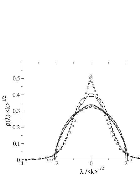
FIG. 1.: Density of eigenvalues of the adjacency matrices of two networks. (i) The classical random graph (the Erdős-Rényi model) with the average degree $\left\langle k\right\rangle=10$: the effective medium (EM) approach (the solid line) and numerical calculations for the graphs of 20 000 vertices [13] (the open circles). (ii) The scale-free random tree-like graph with $\gamma=3$ and the smallest degree $k_{0}=5$: the EM approach (the dashed line), the improved EM approach, see the text (the dashed-dotted line). The results of the simulations of the Barabási-Albert model of 7000 vertices [13] (the open squares). The semicircular law is shown by the thin solid line.

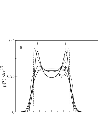
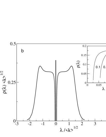
FIG. 2.: Evolution of spectra of a random tree-like graph with the scale-free degree distribution for $\gamma=5$ and the smallest degree $k_{0}=1,2,3$ and 5. The panel $a$ shows the spectra of the graphs with $k_{0}=2,3$ and 5. The dotted line corresponds to the density of eigenvalues of an infinite chain. The dashed and thin solid lines present the spectrum of the $k=3$ and 6 regular Bethe lattices. The panel $b$ shows the spectrum of a random uncorrelated graph having dead-end vertices with the probability $P(1)=0.3$. The insert shows the behavior of  the density of eigenvalues $\rho(\lambda)$ near the dip at $P(1)=0.1,0.2$, and $0.3$. The central peak is produced by localized states.

Scale-free networks. Spectra of scale-free graphs with the degree distribution $P(k)=P_{0}k^{-\gamma}$ differ strongly from the semicircular law [13, 14]. The Barabási-Albert model has a tree-like structure, the exponent $\gamma=3$ of the degree distribution, and negligibly weak correlations between degrees of the nearest neighbors [3]. Therefore, one can assume that the spectrum of a random tree-like graph can mimic well the spectrum of the model. In Fig. 1 we compare the spectrum of the random tree-like graph with $\gamma=3$ and the spectrum of the Barabási-Albert model obtained from simulations [13]. The density of states $\rho(\lambda)$ has a triangular-like form and demonstrates a power-law tail. There is only a noticeable deviation of the EM results from the results of simulations [13] at small eigenvalues $\lambda$.  In order to improve the EM results, we used, as an ansatz, the distribution function $F_{\lambda}(x)=[1+a(\lambda)x^{2}]e^{-ixT(\lambda)}$ instead of the function $F_{\lambda}(x)=e^{-ixT(\lambda)}$. In this case, there are two unknown complex functions $a(\lambda)$ and $T(\lambda)$ which were determined self-consistently from Eq. (23).

Power-law tail. The power-law behavior of the density of eigenvalues $\rho(\lambda)\varpropto\lambda^{-\delta}$ is an important feature of the spectrum of scale-free networks. The simulations [13] of the Barabási-Albert model having the degree exponent $\gamma=3$ revealed a power-law tail of the spectrum, with the eigenvalue exponent $\delta\approx 5$. Our prediction $\delta=2\gamma-1=5$ is in agreement with the result of these simulations.

The study of the topology of the Internet at the Autonomous System (AS) level revealed a power-law behavior of eigenvalues of the associated adjacency matrix [10, 11]. The degree distribution of the network has the exponent $\gamma\approx 2.1$[11]. The eigenvalues $\lambda_{i}$ of the Internet graph are proportional to the power of the rank $i$ of an eigenvalues (starting with the largest eigenvalue): $\lambda_{i}\varpropto i^{\epsilon}$ with some exponent $\epsilon$. This leads to $\rho(\lambda)\varpropto\sum_{i}\delta(\lambda-\lambda_{i})\varpropto\lambda^{-1+1/\epsilon}$. The Multi dataset analyzed in [11] gave $\epsilon\approx-0.447$ and, hence, the eigenvalue exponent $1-1/\epsilon\approx 3.2$. The Oregon dataset [11] gave $\epsilon\approx-0.477$, $1-1/\epsilon\approx 3.1$.

Our results with $\gamma=2.1$ substituted, give the eigenvalue exponent $\delta=2\gamma-1\approx 3.2$ in agreement with the results obtained from empirical data for this network. There are the following reasons for the agreement between the theory for tree-like graphs and the data for the Internet. At first, although the average clustering coefficient of the Internet at AS level is about 0.2, the local clustering coefficient rapidly decreases with increasing the degree of a vertex [36]. In other words, the closest neighborhood of vertices with large numbers of connections is “tree-like”. Recall that vertices with large numbers of connections determine the large-eigenvalue asymptotics of the spectrum. So, we believe that our results for the asymptotics of the spectra of tree-like networks is also valid for the Internet and other networks with similar structure of connections. Secondly, the Internet is characterized by strong correlations between degrees of neighboring vertices [33]. However, as we have shown in the Section VI, such short-range degree correlations do not affect the power-law behavior of eigenvalues.

The study of the Internet topology [11] also revealed a correspondence between the large eigenvalues $\lambda_{i}$ and the degree $k_{i}$: $k_{i}=\lambda_{i}^{2}$. This result is in agreement with our theoretical prediction that it is the highly connected vertices with a degree about $k_{\lambda}\approx\lambda^{2}$  that produce the power-law tail $\rho(\lambda)\varpropto\lambda^{-\delta}$.

The calculations of the eigenvalues spectrum of the adjacency matrix of a pseudofractal graph with $\gamma=2.585\ldots$ [37] have revealed a power-law behavior with $\delta\approx 4.6$. The effective medium approximation gives lower value $\delta=2\gamma-1\approx 4.2$. The origin of the difference is not clear. One should note that the pseudofractal is a deterministically growing graph with a very large clustering coefficient $C=4/5$ and, what is especially important, with long-range correlations between degrees of vertices.

FIG. 3.: Local configurations which produce localized states with zero-eigenvalue (the central peak) in the spectrum of a random graph (see the text).

Weakly connected nodes. Let us study the influence of weakly connected vertices with degrees $1\leqslant k\leqslant 5$ on the spectra of random tree-like graphs with the degree distribution $P(k)=P_{0}k^{-\gamma}$. In Fig. 2$a$ and 2$b$ we represent the evolution of the spectrum of the network with $\gamma=5$, when the smallest degree $k_{0}$ decreases from 5 to 1. The spectra were calculated in the framework of the EM approximation. Similar results are obtained at different $\gamma$. For $k_{0}\leqslant 4$, two peaks at non-zero eigenvalues emerge in the density of states $\rho(\lambda)$. In order to understand an origin of the peaks one can note that for this degree distribution the average degree $\left\langle k\right\rangle$ is close to $k_{0}$. For example, at $k_{0}=3$ we have $\left\langle k\right\rangle=3.49$. Therefore, in this network, the probability to find a vertex having three links is larger than the probability to find a vertex with a degree $k\geqslant 4$. There are large parts of the network which have a local $k=3$–regular structure. In Fig. 2$a$ we show a density of eigenvalues of an infinite $k=3$–regular Bethe lattice [see Eq. (17) at $k=3$]. At small eigenvalues, the density of the regular tree fits well the density of the random network. At large $\lambda$, the density of eigenvalues demonstrates a power-law behavior with the exponent $\delta=2\gamma-1$.

In the case $k_{0}=2$ we have $\left\langle k\right\rangle=2.23$. This network contains long chains which connect vertices with degrees $k\geqslant 3$. In Fig. 2$a$ we display the density of eigenvalues of an infinite chain (see Eq. (17) at $k=2$). At small eigenvalues this density of eigenvalues fits well the density of eigenvalues of the random network. Therefore, it is the vertices with small degrees that are responsible for the formation of density $\rho(\lambda)$ of networks at small eigenvalues.

Dead-end vertices. Let us investigate the effect of dead-end vertices on the spectra of random tree-like graphs with different degree distributions. Fig. 2$b$ shows a spectrum of a scale-free network with $\gamma=5$ and the probability of dead-end vertices $P(1)=0.3$. The EM approximation is used. The spectrum has a flat part and two peaks at moderate eigenvalues. As we have shown above, this (intermediate) part of the spectrum is formed mainly by the vertices with degree $k=2$ and 3. The emergency of a dip at zero is a new feature of the spectrum. In fact, there is a gap in the spectrum obtained in the in the framework of the EM approach. The width of the gap increases with increasing $P(1)$. One can see this in the insert on the Fig. 2$b$. The dead-end vertices also produce a delta peak at $\lambda=0$. The central peak corresponds to localized eigenstates.

Note that the appearance of the central peak and a dip is a general phenomena in random networks with dead-end vertices. We also observed this effect in the classical random graphs. Spectral analysis of the Internet topology on the AS level revealed a central peak with a high multiplicity [16]. Thus the conjecture that localized and extended states are separated in energy may well hold in complex networks. A similar spectra was observed in many random systems, for example, in a binary alloy [38]. In order to estimate the height of the delta peak it is necessary to take into account all localized states. Unfortunately, so far this is an unsolved analytical problem [16]. In Fig. 3 we show local parts of a network, which produce localized states. One can prove that configurations with two and more dead-end vertices, see Fig. 3$a$, produce eigenstates with $\lambda=0$ . The corresponding eigenvectors have non-zero components only at the dead-end vertices [16, 39]. Fig. 3$b$ shows another configuration which produces an eigenstate with the eigenvalue $\lambda=0$. A corresponding eigenvector is localized at vertices 0, 1 and 2.

Finite-size effects. In the present paper we studied the spectral properties of infinite random tree-like graphs. Numerical studies of large but finite random trees demonstrate that the spectrum of a finite tree consists, speaking in general terms, of a continuous component and an infinity of delta peaks. The components correspond to extended and localized states, respectively [17]. There is a hole around each delta peak in the spectrum. A finite regular tree has a spectral distribution function which looks like a singular Cantor function [39]. These results demonstrate that finite size effects in spectra may be very strong. In particular, the finite size of a network determines the largest eigenvalue in its spectrum. As was estimated in the Section V, the largest eigenvalue of the adjacency matrix associated with a scale-free graph is of the order of $k_{cut}^{1/2}=k_{0}^{1/2}N^{1/2(\gamma-1)}$.

Spectrum of the transition matrix. In Fig. 4 we represent a spectrum of the transition matrix $\widehat{P}$ defined by Eq. (53) for a tree-like graph with the scale-free degree distribution $P(k)\varpropto k^{-\gamma}$ at large degrees $k\geqslant 5$. The spectrum was calculated from Eqs. (61) and (62) with the degree exponent $\gamma=2.1$ and the probabilities $P(1),P(2),P(3)$ and $P(4)$ taken from empirical degree distribution of the Internet at the AS level [36].

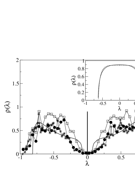
FIG. 4.: Density of eigenvalues of the transition matrix $\widehat{P}$ defined by Eq. (53). (i) The Internet data (the solid circles) and the results of simulations of a random scale-free networks (the open squares) from Ref. [15]. (ii) The spectrum of the Internet extracted from Ref. [16] (the stars). (iii) Our calculations (the solid line) with the degree distribution $P(k)=Ak^{-2.1}$ for $k\geqslant 4$, $P(1)=0.358,$   $P(2)=0.4$   $P(3)=0.12$. These parameters are taken from Ref. [36]. The height of the central peak was estimated from Ref. [16]. The insert shows the spectra of the transition matrix of a random tree-like graph with excluded dead-end vertices: (i) a random tree-like graph with a scale-free degree distribution, $\gamma=3$ , the smallest degree $k_{0}=5$, and $\left\langle k\right\rangle=9.06$ (the dashed line). (ii) A classical random graph with $\left\langle k\right\rangle=9.06$ (the dotted line). (iii) A $k-$regular Bethe lattice with $k=9$ (the solid line).

The spectrum lies in the range $\left|\lambda\right|\leqslant\lambda_{2}<1$. In Fig. 4 we compare our results with the spectrum of the transition matrix $\widehat{P}$ of the Internet obtained in [15, 16]. Unfortunately, the data [15, 16] are too scattered to make a detailed comparison with our results. Nevertheless, one can see that the spectrum of $\widehat{P}$ of the tree-like graph reproduces satisfactory the general peculiarities of the real spectrum. Namely, the spectra have a wide dip at zero eigenvalue and a central delta-peak [16]. The multiplicity of the zero eigenvalue have been estimated in [16]. For a detailed comparison between the spectra, correlations in the Internet must also be taken into account.

In order to reveal an effect of dead-end vertices we calculated spectra of $\widehat{P}$ on a random tree-like graph with the Poisson and the scale-free degree distributions $\gamma=3$ in the case when dead-end vertices are excluded, that is $P(1)=0$, and $\left\langle k\right\rangle=9.06$. These spectra are displayed in the insert on the Fig. 4. In the whole range of eigenvalues these spectra are very close to the spectrum of a $k-$regular Bethe lattice with the degree $k=9.$ These calculations confirm the fact that it is the dead-end vertices that produce the dip in the spectrum of the Internet.

IX Conclusions

In this paper we have studied spectra of the adjacency and transition matrices of random uncorrelated and correlated tree-like complex networks. We have derived exact equations which describe the spectrum of random tree-like graphs, and proposed a simple approximate solution in the framework of the effective medium approach. Our study confirms that spectra of scale-free networks as well as the spectra of classical random graphs do not satisfy the Wigner law.

We have demonstrated that the appearance of a tail of the density of the eigenvalues of sparse random matrices is a general phenomenon. The spectra of classical random graphs (the Erdős-Rényi model) have a rapidly decreasing tail. Scale-free networks demonstrate a power-law behavior of the density of eigenvalues $\rho(\lambda)\propto\left|\lambda\right|^{-\delta}$ . We have found a simple relationship between the degree exponent $\gamma$ and the eigenvalue exponent $\delta$: $\delta=2\gamma-1$. We have shown that correlations between degrees of neighboring vertices do not affect the power-law behavior of eigenvalues. Comparison with the available results of the simulations of the Barabási-Albert model and the analysis of the Internet at the Autonomous System level shows that this relationship is valid for these networks. We found that large eigenvalues $\lambda\gg 1$ are produced by highly connected vertices with a degree $k\approx\lambda^{2}$.

Many real-world scale-free networks demonstrate short-range correlations between vertices [35, 40] and a decrease of a local clustering coefficient with increasing degree of a vertex. Therefore, the relationship $\delta=2\gamma-1$ between the degree-distribution exponent $\gamma$ and the eigenvalue exponent $\delta$ may also be valid for these networks. We can conclude that the power-law behavior $\rho(\lambda)\varpropto\lambda^{-\delta}$ is a general property of real scale-free networks.

Weakly connected vertices form the spectrum at small eigenvalues. Dead-end vertices play a very special role. They produce localized eigenstates with $\lambda=0$ (the central peak). They also produce a dip in the spectrum around the central peak. In conclusion, we believe that our general results for the spectra of tree-like random graphs are also valid for many real-world networks with a tree-like local structure and short-range degree correlations.

REFERENCES

- [1] A.-L. Barabási and R. Albert, Science 286, 509 (1999).
- [2] S.H. Strogatz, Nature 401, 268 (2001).
- [3] R. Albert and A.-L. Barabási, Rev. Mod. Phys. 74, 47 (2002).
- [4] S.N. Dorogovtsev and J.F.F. Mendes, Adv. Phys. 51, 4 (2002).
- [5] M.E.J. Newman, SIAM Review 45, 167 (2003).
- [6] D.J. Watts, Small Worlds: The Dynamics of Networks between Order and Randomness (Princeton University Press, Princeton, NJ, 1999).
- [7] S.N. Dorogovtsev and J.F.F. Mendes, Evolution of Networks: From Biological Nets to the Internet and WWW (Oxford, University Press, 2003).
- [8] D. Cvetković, M. Domb, and H. Sachs, Spectra of Graphs: Theory and Applications (Johann Ambrosius Barth, Heidelberg, 1995); D. Cvetković, P. Rowlinson, and S. Simić, Eigenspaces of graphs (Cambridge University Press, Cambridge, 1997).
- [9] F.R.K. Chung, Spectral Graph Theory (American Mathematical Society, Providence, Rhode Island, 1997).
- [10] M. Faloutsos, P. Faloutsos, C. Faloutsos, Comput. Commun. Rev., 29, 251 (1999).
- [11] G. Siganos, M. Faloutsos, P. Faloutsos, C. Faloutsos, IEEE-ACM T. Network., to appear
- [12] R. Monasson, Eur. Phys. J. B 12, 555 (1999).
- [13] I.J. Farkas, I. Derényi, A.-L. Barabási, and T. Vicsek, Phys. Rev. E 64, 026704 (2001); I. Farkas, I. Derenyi, H. Jeong, Z. Neda, Z.N. Oltvai, E. Ravasz, A. Schubert, A.-L. Barabási, and T. Vicsek, Physica A 314, 25 (2002).
- [14] K.-I. Goh, B. Kahng and D. Kim, Phys. Rev. E 64, 051903 (2001).
- [15] K.A. Eriksen, I. Simonsen, S. Maslov and K. Sneppen, cond-mat/0212001.
- [16] D. Vukadinović, P. Huang, and T. Erlebach, Lect. Notes Comput. Sci. 2346, 83 (2002).
- [17] O. Golinelli, cond-mat/0301437.
- [18] Th. Guhr, A. Müller-Groeling, and H.A. Weidenmüller, Phys. Rep. 299, 189 (1998); A.D. Mirlin, Phys. Rep. 326, 259 (2000).
- [19] A.J. Bray and G.J. Rodgers, Phys. Rev. B 38, 11461 (1988).
- [20] E.P. Wigner, Ann. Math. 62, 548 (1955); 65, 203 (1957); 67, 325 (1958).
- [21] G.J. Rodgers and A.J. Bray, Phys. Rev. B 37, 3557 (1988).
- [22] G. Semerjian and L.F. Cugliandolo, J. Phys. A 35, 4837 (2002).
- [23] A. Bekessy, P. Bekessy, and J. Komlos, Stud. Sci. Math. Hungar. 7, 343 (1972); E.A. Bender and E.R. Canfield, J. Combinatorial Theory A 24, 296 (1978); B. Bollobás, Eur. J. Comb. 1, 311 (1980); N.C. Wormald, J. Combinatorial Theory B 31, 156,168 (1981); M. Molloy and B. Reed, Random Structures and Algorithms 6, 161 (1995).
- [24] S.N. Dorogovtsev, J.F.F. Mendes and A.N. Samukhin, Nucl. Phys. B (2003), cond-mat/0204111.
- [25] M.E.J. Newman, Phys. Rev. Lett. 89, 208701 (2002); J. Berg and M. Lässig, Phys. Rev. Lett. 89, 228701 (2002); S.N. Dorogovtsev, J.F.F. Mendes, and A.N. Samukhin, cond-mat/0206467.
- [26] Note that in a finite Cayley tree, vertices are statistically inequivalent. Indeed, there are vertices deep within the graph and boundary vertices.
- [27] S. Redner, A Guide to First-Passage Processes (Cambridge University Press, Cambridge, 2001).
- [28] M. Mihail and C. Papadimitriou, Lect. Notes Comput. Sci. 254, 2483 (2002).
- [29] R. Solomonoff and A. Rapoport, Bull. Math. Biophys. 13, 107 (1951).
- [30] P. Erdős and A. Rényi, Publ. Math. Debrecen 6, 290 (1959); Publ. Math. Inst. Hung. Acad. Sci. 5, 17 (1960).
- [31] One should note that the position of the cut-off may depend on details of the ensemble of random graphs. In particular, Z. Burda and A. Krzywicki, cond-mat/0207020, showed that the exclusion of multiple connections in a network may diminish .
- [32] M. Krivelevich and B. Sudakov, Combinatorics, Probability and Computing 12, 61 (2003).
- [33] R. Pastor-Satorras, A. Vázquez, and A. Vespignani, Phys. Rev. Lett. 87, 258701 (2001).
- [34] S. Maslov and K. Sneppen, Science 296, 910 (2002).
- [35] E. Ravasz, A.L. Somera, D.A. Mongru, Z.N. Oltvai, and A.-L. Barabási, Science 297, 1551 (2002).
- [36] A. Vázquez, R. Pastor-Satorras and A. Vespignani, Phys. Rev. E 65, 066130 (2002).
- [37] S.N. Dorogovtsev, A.V. Goltsev, and J.F.F. Mendes, Phys. Rev. E 65, 066122 (2002).
- [38] S. Kirkpatrick and T.P. Eggarter, Phys. Rev. B 6, 3598 (1972).
- [39] L. He, X. Liu, and G. Strang, Stud. Appl. Math. 110, 123 (2003).
- [40] A. Vázquez, cond-mat/0211528.
- [41] F. Chung, L. Lu, and V. Vu, Ann. Combinatorics 7, 21 (2003).