Simulation of Interdiffusion in Between Compartments Having Heterogenously Distributed Donors and Acceptors

Abstract

The final stage of latex film formation was simulated by introducing donors and acceptors into the adjacent compartments of a cube. Homogenous and/or heterogeneous donor-acceptor distributions were chosen for different types of simulations. The interdiffusion of the donors and the acceptors within these cubes was generated using the Monte-Carlo technique. The decay of the donor intensity $I(t)$ by direct energy transfer (DET) was simulated for several interdiffusion steps. Gaussian noise was added to the $I(t)$ curves to obtain more realistic decay profiles. $I(t)$ decay curves were fitted to the phenomenological equation to calculate the fractional mixing at each interdiffusion step. The reliability of the Fickian diffusion model in the case of heterogenous and homogeneous donor-acceptor distributions are discussed for latex film formation.

I Introduction

Polymer latex particles have been utilized in a wide variety of applications in the coating and adhesive technologies, biomedical field, information industry and microelectronics. In many of these applications, e.g., coatings and adhesives, latexes form thin polymer films on a substrate surface. Properties (mechanical, optical, transport, etc.) of the final film should be tailor-made according to the application.

Film formation from latex particles is a complicated, multistage phenomenon and depends strongly on the characteristics of colloidal particles. In general, aqueous or non-aqueous dispersions of colloidal particles, with glass transition temperature $(T_{g})$ above the drying temperature, are named hard latex dispersion, however aqueous dispersion of colloidal particles with $T_{g}$ below the drying temperature is called soft latex dispersion. The term ”latex film” normally refers to a film formed from soft particles where the forces accompanying the evaporation of water are sufficient to compress and deform the particles into a transparent, void-free film^1,2. However, hard latex particles remain essentially discrete and undeformed during drying process. Film formation from these dispersion can occur in several stages. In both cases, the first stage corresponds to the wet initial state. Evaporation of solvent leads to second stage in which the particles form a closed pack array, here if the particles are soft they are deformed to polyhedrans (see Figure 1). Hard latex however stay undeformed at this stage. Annealing of soft particles cause diffusion across particle-particle boundaries which leads the film to a homogeneous continuous material. In the annealing of hard latex system, however deformation of particles first leads to void closure^3,4 and then after the voids disappear, diffusion across particle-particle boundaries starts, i.e. the mechanical properties of hard latex films can be evolved by annealing; after all solvent has evaporated and all voids have disappeared.

Figure 1: A pictorial representation of the stages of latex film formation from soft polymer particles. a) The latex dispersion. b) The solvent evaporates leaving the particles in close contact. c) Deformation and packing of the particles. d) Further coalescence produces a mechanically rigid film.

Transmission electron microscopy (TEM) has been used to examine the morphology of dried latex films^5,6. These studies have shown that in some instances the particle boundaries disappeared over time, but in other cases the boundaries persisted for months. It was suggested that in the former case particle boundaries were healed by polymer diffusion across the junction. In the last few years, it has become possible to study latex film formation at the molecular level. Small-angle neutron scattering (SANS) was used to examine deuterated particles in a protonated matrix. It was observed that the radius of the deuterated particle increased in time as the film was annealed⁷ and as the polymer molecules diffused out of the space to which they were originally confined. The process of interparticle polymer diffusion has been studied by the direct energy transfer (DET) method, using transient fluorescence (TRF) measurements^8,9 in conjunction with latex particles labelled with donor and acceptor chromophores. The steady state fluorescence (SSF) method combined with DET was also used for studying film formation from hard latex particles^10-13. An extensive review of the subject is given in reference 14. In DET measurements distribution of donors and acceptors are thought to be crucial i.e. it is believed that donors and acceptors have to be distributed randomly in the latex particles for the reliable TRF measurements, to determine the diffusion coefficients, D of polymer chains.

Recently we have performed various experiments with photon transmission method using an U.V. Visible (UVV) spectrophotometer to study latex film formation from PMMA and PS latexes in where void closure and interdiffusion processes at the junction surfaces are studied^15-18. All these studies indicate that annealing leads to polymer diffusion and mixing as the particle junction heals during latex film formation. Recently, Monte Carlo simulation of interdiffusion and its monitoring by DET during latex film formation has also been studied in our laboratories^19,20.

In this work, Monte Carlo method was used to simulate the final stage of film formation by introducing donors and acceptors into the adjacent compartments of a cube. Four different combinations of donor-acceptor distributions were chosen for the different types of simulations. For example in the first case distribution of donors and acceptors in their adjacent compartments are taken as homogenous and gaussian respectively. In the second case distributions are switched from one compartment to the other. In the third case, both distributions are taken as gaussian and in the final case, distribution of donors and acceptors are both taken homogeneously to compare this case with the others.

The interdiffusion of donors and acceptors between these adjacent compartments was randomly generated by Monte Carlo method. The decay of the donor intensity, $I(t)$ by DET was simulated for several interdiffusion steps and a gaussian noise was added to generate the realistic time resolved fluorescence data. I(t) decays were fitted to the phenomenological equation to obtain the fractional mixing at each interdiffusion step. The reliability of the Fickian model and the effect of heterogenous donor-acceptor distributions are discussed at the last stage of latex film formation process.

II DET and Fluorescence Decay

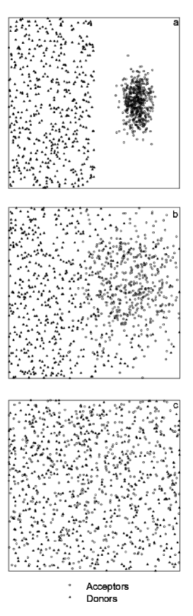
Figure 2: Several snapshots of the interdiffusion process between adjacent compartments of a cube in which donors and acceptors are distributed homogenous and gaussian wise. a) K=0.0, b) K=0.3 and c) K=1.0  .

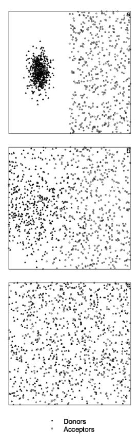
Figure 3: Several snapshots of the interdiffusion process between adjacent compartments of a cube in which donors and acceptors are distributed gaussian and homogenous wise. a) K=0.0, b) K=0.3 and c) K=1.0  .

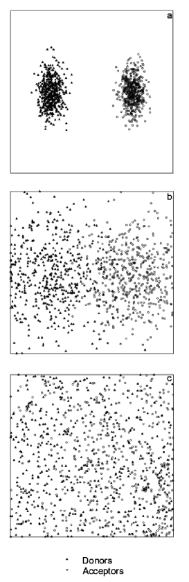
Figure 4: Several snapshots of the interdiffusion process between adjacent compartments of a cube in which both donors and acceptors are distributed gaussian wise. a) K=0.0, b) K=0.3 and c) K=1.0  .

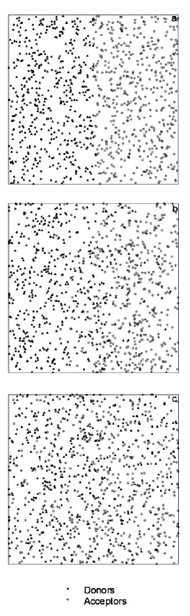
Figure 5: Several snapshots of the interdiffusion process between adjacent compartments of a cube in which both donors and acceptors are distributed homogenously. a) K=0.1, b) K=0.4 and c) K=1.0  .

Polymer diffusion obeys de Gennes scaling laws for times short compared to the tube renewal time $t_{tr}$, but for long times it is like a random walk process (Fickian diffusion). In order to be able to determine whether the diffusion is Fickian, one must compare the experimental data with the results of simulations of DET with Fickian diffusion.

TRF in conjunction with the DET method, monitors the extent of interdiffusion of donor (D) and the acceptor (A) labelled polymer molecules. The sample is made of a mixture of D and A labelled latex spheres. When this sample is annealed for a period of time and the donor fluorescence profiles are measured, each decay trace provides a snapshot of the extent of interdiffusion⁹. A film sample after annealing was considered to be composed of three regions; unmixed D, unmixed A and the mixed D - A region. This model was first empirically introduced by the two component donor flourescence decay^21,22.

When donor dyes are excited using a very narrow pulse of light, the excited donor returns to the ground state either by emitting a fluorescence photon or through the nonradiative mechanism. For a well behaved system, after exposing the donors with a short pulse of light, the fluorescence intensity decays exponentially with time. However, if acceptors are present in the vicinity of the excited donor, then there is a possibility of DET from the excited donor to the ground state acceptors. In the classical problem of DET, neglecting back transfer, the probability of the decay of the donor at $r_{k}$ due to the presence of an acceptor at $r_{i}$ is given by²³

$$P_{k}(t)=exp[-t/{\tau_{0}}-{w_{ik}}t]$$ (1)

where $w_{ik}$ is the rate of energy transfer given by Förster as

$$w_{ik}={\frac{3}{2}}{{\kappa}^{2}}{\frac{1}{{\tau}_{0}}}{({\frac{R_{0}}{r_{ik}}})}^{6}$$ (2)

Here $R_{0}$ represents the critical Förster distance and $\kappa$ is a dimensionless parameter related to the geometry of interacting dipole. If the system contains $N_{D}$ donors and $N_{A}$ acceptors, then the donor fluorescence intensity decay can be derived from the equation (2) and given by¹⁶

$$\frac{I(t)}{I(0)} = \exp(-t/{\tau_{0}})\frac{1}{N_{D}}\int{{n_{D}}(r_{k})dr_{k}}$$ (3)

$$\times\prod_{i=1}^{N_{A}}{\frac{1}{N_{A}}}\int{{n_{A}}{(r_{i})}}dr_{i}\exp{(-w_{ik}t)}$$

Here $n_{D}$ and $n_{A}$ represent the distribution functions of donors and acceptors. In the thermodynamic limit equation (3) becomes¹⁶

$$\frac{I(t)}{I(0)} = \exp(-t/{\tau_{0}})\frac{1}{N_{D}}\int{{n_{D}}(r_{k})dr_{k}}$$ (4)

$$\times\exp({-\int{n_{A}(r_{i})dr_{i}(1-\exp{(-{w_{ik}}t))}}})$$

This equation can be used to generate donor decay profiles by Monte-Carlo techniques. It is shown that the equation (4) reduces to a more simple form which can be compared to the experimental data³. Their argument is summarized below for clarity. Changing to the coordinate $r_{ik}=r_{i}-r_{k}$ leads to,

$$\frac{I(t)}{I(0)} = \exp(-t/{\tau_{0}})\frac{1}{N_{D}}\int{{n_{D}}(r_{k})dr_{k}}$$ (5)

$$\times \prod_{i=1}^{N_{A}}\int_{r_{K}}^{R_{g}-r_{K}}{{n_{A}}{({r_{ik}}+r_{k})}}dr_{ik}\exp{(-w_{ik}t)}$$

where $R_{g}$ is an arbitrary upper limit. Placing a particular donor at the origin and assuming that the mixed and unmixed regions are created during interdiffusion of D and A, the equation (5) becomes

$$\frac{I(t)}{I(0)} = B_{1}\exp(-t/{\tau_{0}})\prod_{i=1}^{N_{A}}\frac{1}{N_{A}}\int_{0}^{R_{g}}{{n_{A}}(r_{ik})dr_{ik}}$$ (6)

$$\times\exp{({-w_{ik}}t)}+B_{2}\exp(-t/{\tau_{0}})$$

where

$$B_{1,2}=\frac{1}{N_{D}}\int_{1,2}{n_{D}(r_{k})dr(k)}$$ (7)

represent the fraction of donors in mixed and unmixed regions, respectively. The integral in equation (6) produces a Förster type of function^24,25

$$\prod_{i=1}^{N_{A}}\frac{1}{N_{A}}\int_{0}^{R_{g}}n_{A}(r_{ik})dr_{ik}exp(-w_{ik}t)=exp(-C({\frac{t}{\tau_{0}}})^{1/2})$$ (8)

where C is proportional to acceptor concentration. Eventually, one gets the following formula for the fluorescence intensity.

$$\frac{I(t)}{I(0)}=B_{1}\exp(-t/{\tau_{0}}-C(\frac{t}{\tau_{0}})^{1/2})+B_{2}\exp(-t/{\tau_{0}})$$ (9)

Here it is useful to define the mixing ratio K representing the order of mixing during interdiffusion of the donors and the acceptors as

$$K=\frac{B_{1}}{B_{1}+B_{2}}$$ (10)

III Simulation of Interdiffusion

The interdiffusion of donors and acceptors between two adjacent compartments corresponds to the last stage of latex film formation process. Here the geometry is simplified using cubes instead of the polyhedrons, and donors and acceptors are randomly distributed in seperate adjacent compartments in a cube. Figure 2a, 3a, 4a and 5a present the four types of combinations of donor-acceptor distributions. In Figure 2a donors and acceptors are distributed in the adjacent compartments in homogeneous and gaussian wise distributions, respectively. When these distributions are completely inversed, the situation is presented in Figure 3a. Figures 4a and 5a present acceptors and donors both distributed in separate compartments in gaussian and in homogeneous wise distributions, respectively.

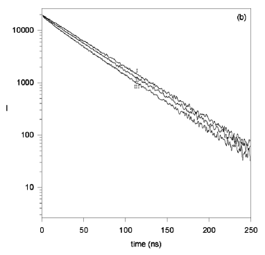
Figure 6: a) Decay curves at the several interdiffusion steps for both donors and acceptors are homogenous distributed in adjacent compartments. I) K=0.1, II) K=0.5, III) K=1.0 b) Noisy decay curves for the above picture.

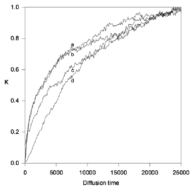
Figure 7: Comparison of the plots of the mixing ratio K versus diffusion time for different initial distributions as a) Donors and acceptors are distributed homogenous and gaussian wise, b) Donors and acceptors are distributed gaussian and homogenous wise, c) Both donors and acceptors are distributed gaussian wise, d) Both donors and acceptors are distributed homogenously.

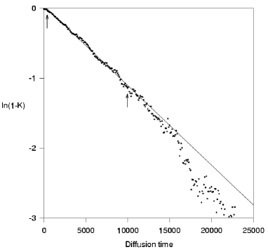
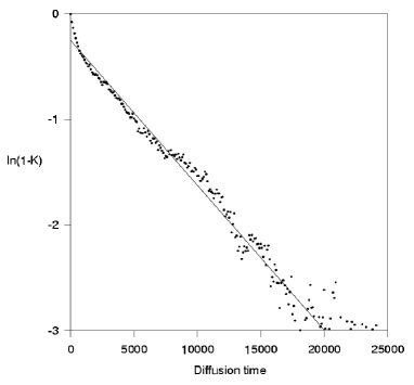
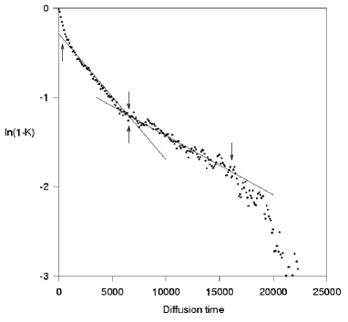
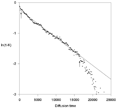
Figure 8: The plots of $\ln(1-K)$ versus diffusion time obtained for different combinations of distributions given in Figure 7. The solid lines present the fit of the data to equation (19). The slope of the solid lines produced diffusion constants which are listed in Table I. The regions used for the linear fits are shown within arrows in Figures 8a, 8c and 8d. In Figure 8b all the data points are used in the fit.

Figures 2b, 3b, 4b and 5b present the picture after the Brownian motion of donors and acceptors generated for several interdiffusion steps for each combination of donor-acceptor pairs which are given in Figures 2a, 3a, 4a and 5a, respectively. In each diffusion step, all the donors and acceptors move within a range of 0 to 1 $A^{o}$ in any direction, but are reflected from the sides of the cube. After each diffusion step, the diffusion time increments one unit. $25\times 10^{3}$ diffusion steps were used for all sample simulations. The decay of donor intensity by DET is simulated for the configurations at the end of each 100 step of diffusion, therefore the diffusion process can be monitored quite clearly and accurately. Moreover, the average is taken over 10 different runs for each initial distribution. Figures 2c, 3c, 4c and 5c present the final picture of the interdiffusion between two adjacent compartments in a cube.

The donor decay profiles were generated using equation (4). The side of the cube, L, is taken as 500 $A^{o}$ and the Förster distance as 26 $A^{o}$. The number of donors, $N_{D}$, and acceptors $N_{A}$, are both chosen as 500. The $w_{ik}$ values for each donor-acceptor pair are obtained from equation (2). The parameter $\kappa^{2}$ is chosen as 0.476, a value appropriate for immobile dyes²⁰, and the donor lifetime $\tau_{d}$ is taken as 44ns. Equation (4) is then used to simulate the donor intensity I(t) decay profiles. $I(0)=2\times 10^{4}$ is chosen and the decay profiles are obtained for a 250ns interval, divided into 250 channels of 1ns each. Decay profiles at the several interdiffusion steps for both donors and acceptors are homogenously distributed in adjacent compartments are presented in Figure 6a.

Here, one may also take into account the effect of the lamp profile when calculating the decay profiles^19,20. To do so the decay profiles generated by the Monte Carlo simulation should be convolved with an experimental lamp profile, then the experimentally measured $\phi(t)$ is obtained by convolution of $I(t)$ with the instrument response function $L(t)$, as

$$\phi(t)=\int_{0}^{t}L(t)I(t-s)ds$$ (11)

In this work, since we are interested in the effect of donor-acceptor distributions on the interdiffusion, instead of using experimental decay profiles we used generated decay profiles. This assumption is valid if one uses a delta, $\delta$ function light source (e.g. a very fast laser) as the lamp profile. In this case no convolution is needed and equation (11) produces $I(t)$. However, to obtain more realistic decay profiles, gaussian noise can be added to the original decay profiles using Box, Muller and Marsaglia²⁴ algorithm. In this algorithm, at first two gaussian numbers ( $U_{1}$ , $U_{2}$ ) between $0$ and $1$ are created. Then $V_{1}$ and $V_{2}$ are calculated as shown below

$$V_{1}=2U_{1}-1$$ (12)

$$V_{2}=2U_{2}-1$$ (13)

Both $V_{1}$ and $V_{2}$ are distributed randomly in the range $[-1,1]$. S is calculated from these two numbers.

$$S={{V_{1}}^{2}}+{{V_{2}}^{2}}$$ (14)

If $S<1$, operation is unsuccessful and new $U_{1}$ and $U_{2}$ numbers are created. If $S>1$, $X_{1}$ and $X_{2}$ are calculated as shown below.

$$M = q(\frac{-2\ln S}{S})^{\frac{1}{2}}$$ (15)

$$X_{1} = (V_{1}M)+p$$ (16)

$$X_{2} = (V_{2}M)+p$$ (17)

$X_{1}$ and $X_{2}$ are mutually independent. They are gaussian numbers with an average p and standard deviation q. The noisy decay profiles for the homogenously distributed donors and acceptors at several interdiffusion steps are shown in Figure 6b.

In order to calculate the mixing ratio, K defined in equation (10) one should fit the generated decay profiles to equation (9). The decay profiles were fitted to equation (9) using Levenberg-Marquart²⁵ algorithm. During fits the parameters C and $\tau_{0}$ are kept constant (C=1) and only the parameters $B_{1}$ and $B_{2}$ are varied. More than $5000$ decay profiles are fitted and the goodness of fitting is varied around $\chi^{2}<1.5$. The produced $B_{1}$ and $B_{2}$ values are used to obtain K values at each interdiffusion step. Figure 7 compares the plots of K versus diffusion time for the interdiffusions presented in Figures 2, 3, 4 and 5. Each curve in Figure 7 is obtained from the average of a set of 10 runs.

To test whether the simulated interdiffusion is Fickian or not, the planar sheet model is chosen²⁶. In this model the fraction of the diffusing substance that has diffused out of the planar sheet at time t is given by

$$K_{s}=\frac{8}{\pi}\sum_{n=0}\frac{1}{{(2n+1)}^{2}}\exp{(-\frac{D{(2n+1)}^{2}\pi^{2}t}{a^{2}})}$$ (18)

where D is the diffusion constant and a is the maximum distance over which diffusion can occur. Since $\lim_{k\rightarrow\infty}K_{s}=1$, eq.(18) can be written for $n=0$ in the form

$$\ln(1-K_{s})=-\frac{D\pi^{2}t}{a^{2}}$$ (19)

$\ln(1-K)$ values are plotted versus diffusion time in Figure 8 and were fitted to equation (19). The fits obtained for all of the four combinations of distributions are shown in Figures 8a, 8b, 8c and 8d. The solid lines in the plots represent the fitting curve and the dots represent the digitized data. The diffusion constants and the correlation coefficients showing the goodness of fits are presented in Table I.

Table 1: $D\pi^{2}/a^{2}$ values are produced by fitting the data in Figure 7 to the equation (19). The fits are presented in Figure 8 for the various combinations of distributions. $R^{2}$ is the correlation coefficient for the fits.

Donor	Acceptor	${\bf D\pi^{2}/a^{2}(\times 10^{-4})}$	${\bf R^{2}}$
Homogenous	Gaussian	1.14 $\pm$ 0.01	0.995
Gaussian	Homogenous	1.37 $\pm$ 0.03	0.925
Gaussian	Gaussian	1.41 $\pm$ 0.03	0.973
		0.66 $\pm$ 0.02	0.958
Homogenous	Homogenous	0.91 $\pm$ 0.01	0.991

IV Conclusions

Fits in Figure 8 and the values in Table I strongly suggest that people who work in TRF area have to be very careful to synthesize their latex particles which are labelled with the fluorescence dyes. In this work, it is observed that when the dye distribution is not homogenous different results in interdiffusion processes can be produced even the latex particles are in equal size. All data in Figure 8 present that interdiffusion saturates at the long time region. At the short time region the initial donor-acceptor distribution is quite critical and effects the interdiffusion (mixing ratio, K). When donors are distributed in gaussian wise, delay for the onset of interdiffusion is observed at early time region which is obvious, since it takes some time for the donors to reach the acceptors to perform DET. In this case if the acceptors are distributed homogenously, interdiffusion occurs with a single diffusion constant D, however if the acceptors are distributed gaussian wise, two different interdiffusion regimes can be observed at the intermediate time region. In other words, after a certain delay at early times, donors and acceptors meet quite fast to perform DET and then interdiffusion slows down and finally mixing saturates at longer times.

When the donors are distributed homogenously the delay at the short time region is quite small, especially if the acceptors are distributed gaussian wise, no delay is observed. In this case when the acceptors are distributed either gaussian or homogenous wise, single interdiffusion regime is observed at intermediate time region where in both cases interdiffusion rate is similar and much smaller than when the donors are distributed gaussian wise (see Table I).

In conclusion, if one assumes that the ideal distribution for donors and acceptors in latex particles are both homogenous, then one has to expect that experimental results for K should obey the picture in Figure 8d, even though the picture in Figure 8a looks much better i.e. interdiffusion starts with no delay and produces single interdiffusion constant.

References

- [1] S. T. Eckersley and A. Rudin, J. Coatings Technol. 62, No.780, 89 (1990).
- [2] M. Joanicot, K. Wong, J. Maquet, Y. Chevalier, C. Pichot, C. Graillat, P. Linder, L. Rios and B. Cabane, Prog. Coll. Polym. Sci. 81, 175 (1990).
- [3] P. R. Sperry, B. S. Snyder, M. L. O’ Downd and P. M. Lesko, Langmuir, 10, 2619 (1994).
- [4] J. K. Mackenzie and R. Shuttleworth, Proc. Phys. Soc. 62, 838 (1946).
- [5] J. W. Vanderhoff, Br. Polym. J., 2. 161 (1970).
- [6] D. Distler and G. Kanig, Colloid Polym. Sci., 256, 1052 (1978).
- [7] K. Kahn, G. Ley, H. Schuller and R. Oberthur, Colloid Polym. Sci., 66, 631 (1988).
- [8] M. A. Winnik, Y. Wang and F. Haley, J. Coatings Technol., 64, 51 (1992).
- [9] Ö. Pekcan, M. A. Winnik and M. D. Croucher, Macromolecules, 23, 2673 (1990).
- [10] M. Canpolat and Ö. Pekcan, J. Polym. Sci. Polym. Phy. Ed., 34, 691 (1996).
- [11] M. Canpolat and Ö. Pekcan, Polymer, 36, 4433 (1995).
- [12] Ö. Pekcan and M. Canpolat, J. App. Polym. Sci., 59, 277 (1996).
- [13] M. Canpolat and Ö. Pekcan, Polymer, 36, 2025 (1995).
- [14] Ö. Pekcan, Trends in Polymer Science, 2, 236 (1994).
- [15] Ö. Pekcan, F. Kemeroğlu and E. Arda, Eur. Polym. J., 34, 1371 (1998).
- [16] Ö. Pekcan, F. Kemeroğlu, J. App. Polym. Sci. (in press)
- [17] Ö. Pekcan, E. Arda, K. Kesenci and E. Pişkin, J. App. Polym. Sci., 68, 1257 (1998).
- [18] Ö. Pekcan, E. Arda, J. App. Polym. Sci., 70, 339 (1998).
- [19] K. S. Güntürk, A. T. Giz and Ö. Pekcan, Eur. Polym. J., 34, 789 (1998).
- [20] K. S. Güntürk, A. T. Giz and Ö. Pekcan, Polymer, 39, 10 (1998).
- [21] M. A. Winnik, Ö. Pekcan, M. D. Croucher, “Scientific Methods for the Study of Polymer Colloids and their Applications”, Eds. F. Condon, R. H. Otterwell, NATO ASI, Kluver Acad. Pub. (1988).
- [22] Y. Wang and M. A. Winnik, Macromolecules 26, 3147 (1993).
- [23] T. H. Förster, Ann. Phys., 2, 55 (1948).
- [24] H. William, A. Tenkolsky, T. Vetterling, P. Flannery, eds., “Numerical Recipes in C 2nd ed.”, Cambridge University Press (1992).
- [25] J. Klafter and A. Blumen, J. Chem. Phys., 80, 875 (1984).
- [26] J. Bauman and M. D. Fayer, J. Chem. Phys., 85, 408 (1986).