Steady states of a $\chi^{3}$ parametric oscillator with coupled polarisations

Abstract

Polarisation effects in the microcavity parametric oscillator are studied using a simple model in which two $\chi^{3}$ optical parametric oscillators are coupled together. It is found that there are, in general, a number of steady states of the model under continuous pumping. There are both continuous and discontinuous thresholds, at which new steady-states appear as the driving intensity is increased: at the continuous thresholds, the new state has zero output intensity, whereas at the discontinuous threshold it has a finite output intensity. The discontinuous thresholds have no analog in the uncoupled device. The coupling also generates rotations of the linear polarisation of the output compared with the pump, and shifts in the output frequencies as the driving polarisation or intensity is varied. For large ratios of the interaction between polarisations to the interaction within polarisations, of the order of 5, one of the thresholds has its lowest value when the pump is elliptically polarised. This is consistent with recent experiments in which the maximum output was achieved with an elliptically polarised pump.

I Introduction

Semiconductor microcavities are high finesse Fabry-Perot structures, typically consisting of a planar semiconductor cavity layer bounded by Bragg mirrors. The mirrors confine two-dimensional photons, which mix with the exciton states of quantum wells embedded in the cavity. Such mixing gives a type of two-dimensional polariton known as a “cavity polariton”review1 . The non-linear dynamics of cavity polaritons corresponding to polariton-polariton scattering has been extensively studied, due to the possibility of observing bosonic effects such as stimulated scattering. Recent experiments have demonstrated new aspects to the non-linear dynamics of coherent polaritons: parametric oscillation and amplification.

Parametric oscillation and amplification in microcavities has been demonstrated using both pulsedsavvidis2000 ; erland2001 and continuous-wavestevenson2000 excitation. In these experiments, a laser tuned near to the energy of the lower polariton mode is used to generate a coherent polariton field in the microcavity. Owing to a $\chi^{(3)}$ non-linearity provided by the exciton-exciton interaction, this pump mode is coupled to “signal”and “idler” modes at lower and higher energies. The coupling corresponds to the scattering of pairs of pump polaritons into the signal and idler, in contrast to the coupling in the conventional $\chi^{(2)}$ optical parametric oscillatorshen , which corresponds to the fission of pump photons. Above a critical pump intensity, the gain due to the nonlinearity outweighs the damping of the signal and idler modes. When this occurs, the steady-state in which there is a single coherent field at the pump becomes unstable towards a state which also has coherent fields at the signal and idler. In the continuously pumped experiments, this instability develops spontaneously, and the new steady-state is reached. In the pulsed experiments of Ref.  savvidis2000, however, there is not enough time for the instability to develop spontaneously before the excitation pulse is over. Instead it is triggered using a second “seed” laser pulse injected into the signal mode.

The theory of microcavity parametric oscillation and amplification was initially developed by Ciuti et al.ciuti2000 and Whittakerwhittaker2001 . In the former, the pulsed measurements of Ref. savvidis2000, are treated within a quantum optics formalism, while the latter used classical nonlinear optics to explain the steady-state behaviour. The dynamical equations which occur in both models are the same, demonstrating that the phenomena are essentially classical effects, with the exception of the incoherent luminescence which occurs below threshold.ciuti2001 More recent theoretical work by Savasta et al.savasta2003 includes frequency-dependent nonlinearities and nonlinear absorption, arising from exciton-exciton correlations.

Parametric oscillation requires a significant electromagnetic response at the wavevectors and frequencies of the signal and idler. Thus the signal and idler must lie near the polariton dispersion. The signal and idler must also satisfy the requirements of wavevector and frequency conservation in the generation process. In the conventional parametric oscillator, these two requirements are usually met by exploiting birefringenceshen . Thus the polarisations of the fields for which the device operates are prescribed. In the microcavity parametric oscillator however, the unusual dispersion of cavity polaritons allows them to be met irrespective of the polarisations. This is achieved for pump fields near to a particular “magic” wavevector. In this paper we study the effects of these polarisation degrees-of-freedom.

There are two recent experiments on the polarisation effects in microcavities that are resonantly pumped near to the magic wavevector, one using continuous wave excitationtartakovskii2000 , and one using pulsed excitationlagoudakis2002 . Both these papers argue that their observations imply the existence of interactions between polaritons of different circular polarisations. While some aspects of the pulsed datalagoudakis2002 were recently explained using a model without such interactionskavokin2003 , they may still be necessary to understand the steady-state experiments of Ref. tartakovskii2000, . Furthermore, interactions between polaritons of different polarisations seem to be necessary to explain the polarisation dependence of four-wave mixing experiments in microcavitieskuwata-gonokami1997 . They could originate from interactions between excitons of different polarisations, which have been used to explain the polarisation dependence of four-wave mixing in quantum wellsbott1993 ; maialle1994 .

Because the parametric oscillator involves the dynamics of coherent polaritons, and not simply scattering, the consequences of an interaction between polaritons of different polarisations are not obvious. In this paper, we investigate the effects of polarisation coupling on the steady-states of a simple model.

The remainder of this paper is organised as follows. In section II we present the model. In section III we explore the steady-states of the model. The steady-state calculation is subdivided: in section III.1 we calculate the possible values of the pump polariton fields, in section III.2 we calculate the output fields for those values of the pump fields, and in section III.3 we combine these results with the “pump depletion” equations to determine the behaviour for a particular external drive. In section IV we qualitatively compare our results with the continuously pumped experiments reported in Ref. tartakovskii2000, , and comment on the stability of our solutions and possible microscopic origins for our phenomenological coupling. Finally, section V summarises our conclusions.

II Model

The model we analyse in this paper is a generalisation of the scalar treatment described in Ref. whittaker2001, . That model considers the scattering between pump, signal and idler polaritons of one circular polarisation. The exciton amplitudes in these fields are denoted by $p_{\uparrow}$, $s_{\uparrow}$and $i_{\uparrow}$. They are time dependent, so the exciton field at the pump wavevector ${\rm\bf k_{p}}$, for example, takes the form $\mbox{$p_{\uparrow}$}(t)\exp{\mbox{$\rm i$}({\rm\bf k_{p}}.{\bf r}-\mbox{$\omega_{p}^{0}$}t)}$, where $\omega_{p}^{0}$ is the lower branch polariton frequency. For simplicity, we assume that the bare polariton frequencies satisfy the triple resonance condition $2\omega_{p}^{0}=\omega_{s}^{0}+\omega_{i}^{0}$. We also assume that the time dependence of the amplitudes is slow compared with the polariton splitting, so the upper branch can be omitted from the model. The scattering is modelled by a term proportional to $|\mbox{$\phi_{\uparrow}$}|^{4}$ in the Lagrangian density, corresponding to a $\chi^{(3)}$ nonlinearity. The equations governing the exciton amplitudes are then

$$-\frac{\mbox{$\rm i$}}{\mbox{$|\mbox{\scriptsize{\it X}}_{p}|$}^{2}}\left(\frac{d}{dt}+\mbox{$\gamma_{p}$}\right)\mbox{$p_{\uparrow}$}+2\mbox{$\kappa$}\mbox{$s_{\uparrow}$}\mbox{$i_{\uparrow}$}\mbox{$p_{\uparrow}^{*}$} = \frac{\mbox{$\mbox{\scriptsize{\it C}}_{p}$}}{\mbox{$\mbox{\scriptsize{\it X}}_{p}$}}\mbox{$f_{\uparrow}$}(t)$$ (1a)

$$-\frac{\mbox{$\rm i$}}{\mbox{$|\mbox{\scriptsize{\it X}}_{s}|$}^{2}}\left(\frac{d}{dt}+\mbox{$\gamma_{s}$}\right)\mbox{$s_{\uparrow}$}+\mbox{$\kappa$}\mbox{$p_{\uparrow}$}^{2}\mbox{$i_{\uparrow}^{*}$} = 0$$ (1b)

$$-\frac{\mbox{$\rm i$}}{\mbox{$|\mbox{\scriptsize{\it X}}_{i}|$}^{2}}\left(\frac{d}{dt}+\mbox{$\gamma_{i}$}\right)\mbox{$i_{\uparrow}$}+\mbox{$\kappa$}\mbox{$p_{\uparrow}$}^{2}\mbox{$s_{\uparrow}^{*}$} = 0$$ (1c)

Here $\gamma_{p}$ etc are the homogeneous line widths of the polariton states, and $\mbox{\scriptsize{\it C}}_{p}$ and $\mbox{\scriptsize{\it X}}_{p}$ are the amplitudes of the photon and exciton in the polariton, i.e. the Hopfield coefficients. They appear because it is only the excitonic part of the polariton which interacts. $\mbox{$f_{\uparrow}$}(t)$ is the external driving field for the pump, in a frame rotating at the appropriate polariton frequency. For the continuously pumped situation we consider in the present paper, $\mbox{$f_{\uparrow}$}(t)=f_{\uparrow}\exp(-i\delta_{p}t)$, where $\delta_{p}$ is the pump detuning. The nonlinear term in the pump equation (1a) describes the scattering of pairs of polaritons out of the pump field, while the terms in (1b,1c) provide the corresponding growth in the signal and idler fields. The nonlinear exciton blue-shiftciuti2000 ; whittaker2001 is neglected for simplicity.

To incorporate the polarisation degrees-of-freedom, we introduce pump, signal and idler fields for the other circular polarisation, denoting their exciton amplitudes by $p_{\downarrow}$, $s_{\downarrow}$and $i_{\downarrow}$. Without any coupling terms, their dynamics is given by the analogs of (1). However, we now introduce a second $\chi^{(3)}$ excitonic nonlinearity which couples the up and down spin excitons. Rather than derive a realistic microscopic model of exciton spin scattering, we treat this phenomenologically by choosing the simple form $\mbox{$g$}_{0}|\mbox{$\phi_{\uparrow}$}|^{2}|\mbox{$\phi_{\downarrow}$}|^{2}$. We assume that the coefficients $\kappa$ and $\mbox{$g$}_{0}$ are independent of momentum and energy. While the former is physically justified because the wavelengths of the polaritons which scatter are much larger than any excitonic length scaleciuti2000 , it is more difficult to rule out the possibility of an energy dependent process.

The interaction between excitons of opposite spins introduces two new types of polariton scattering terms into the equations of motion. If $\mbox{$g$}_{0}$ is constant as we assume these both have the same strength, $\mbox{$g$}_{0}$, but for now we add subscripts in order to distinguish the processes in Eqs. 2. The first process we describe as cross-polarisation parametric scattering, where a pair of pump polaritons of opposite polarisation scatter into a signal and idler modes, also of opposite polarisation. These terms are written with a coefficient $g_{c}$. The second process we describe as a polarisation-flip, where a pump and signal, or idler, polariton exchange polarisations. This flip process is given a strength $g_{s}$. A similar flip process can also occur between signal and idler polaritons, but this possibility is neglected here, making the assumption that the signal and idler amplitudes are small compared with that of the pump.

With these polarisation-coupling terms, the equations for the spin-up fields are

$$-\frac{\mbox{$\rm i$}}{\mbox{$|\mbox{\scriptsize{\it X}}_{p}|$}^{2}}\left(\frac{d}{dt}+\mbox{$\gamma_{p}$}\right)\mbox{$p_{\uparrow}$}+2\mbox{$\kappa$}\mbox{$s_{\uparrow}$}\mbox{$i_{\uparrow}$}\mbox{$p_{\uparrow}^{*}$}+\mbox{$g_{c}$}(\mbox{$s_{\downarrow}$}\mbox{$i_{\uparrow}$}+\mbox{$s_{\uparrow}$}\mbox{$i_{\downarrow}$})\mbox{$p_{\downarrow}^{*}$}+\mbox{$g_{s}$}(\mbox{$s_{\uparrow}$}\mbox{$s_{\downarrow}^{*}$}+\mbox{$i_{\uparrow}$}\mbox{$i_{\downarrow}^{*}$})\mbox{$p_{\downarrow}$} = \frac{\mbox{$\mbox{\scriptsize{\it C}}_{p}$}}{\mbox{$\mbox{\scriptsize{\it X}}_{p}$}}f_{\uparrow}\exp(-i\delta_{p}t),$$ (2a)

$$-\frac{\mbox{$\rm i$}}{\mbox{$|\mbox{\scriptsize{\it X}}_{s}|$}^{2}}\left(\frac{d}{dt}+\mbox{$\gamma_{s}$}\right)\mbox{$s_{\uparrow}$}+\mbox{$\kappa$}\mbox{$p_{\uparrow}$}^{2}\mbox{$i_{\uparrow}^{*}$}+\mbox{$g_{c}$}\mbox{$p_{\uparrow}$}\mbox{$p_{\downarrow}$}\mbox{$i_{\downarrow}^{*}$}+\mbox{$g_{s}$}\mbox{$p_{\uparrow}$}\mbox{$p_{\downarrow}^{*}$}\mbox{$s_{\downarrow}$} = 0,$$ (2b)

$$-\frac{\mbox{$\rm i$}}{\mbox{$|\mbox{\scriptsize{\it X}}_{i}|$}^{2}}\left(\frac{d}{dt}+\mbox{$\gamma_{i}$}\right)\mbox{$i_{\uparrow}$}+\mbox{$\kappa$}\mbox{$p_{\uparrow}$}^{2}\mbox{$s_{\uparrow}^{*}$}+\mbox{$g_{c}$}\mbox{$p_{\uparrow}$}\mbox{$p_{\downarrow}$}\mbox{$s_{\downarrow}^{*}$}+\mbox{$g_{s}$}\mbox{$p_{\uparrow}$}\mbox{$p_{\downarrow}^{*}$}\mbox{$i_{\downarrow}$} = 0.$$ (2c)

The equations obeyed by the spin-down fields are given by flipping the spin labels in Eqs. 2.

In what follows we will not be concerned with the absolute intensities of the fields or external pumps. This allows us to eliminate the normal coupling $\kappa$ by scaling all the fields and the pumps according to $\frac{\mbox{$\mbox{\scriptsize{\it C}}_{p}$}}{\mbox{$\mbox{\scriptsize{\it X}}_{p}$}}f_{\uparrow}\to\frac{\mbox{$\mbox{\scriptsize{\it C}}_{p}$}}{\mbox{$\mbox{\scriptsize{\it X}}_{p}$}}f_{\uparrow}\sqrt{\mbox{$\kappa$}}=F_{\uparrow}$, and $\mbox{$p_{\uparrow}$}\to\mbox{$p_{\uparrow}$}/\sqrt{\mbox{$\kappa$}}$ etc.. After this rescaling, the coupling strengths in (2) are replaced by their ratios to $\kappa$: $\mbox{$g_{c}$}\to\mbox{$g_{c}$}/\mbox{$\kappa$}=\mbox{$g$}$ etc.

III Parametric Oscillation

For particular amplitudes of the pump fields, equations 2b and 2c admit harmonic solutions with finite amplitudes for the signal and idler fields. To find these steady states, we set $\mbox{$p_{\uparrow}$}(t)=\mbox{$p_{\uparrow}$}\exp{(-i\delta_{p}t)}$ etc. When the detunings obey

$$2\delta_{p}=\delta_{s}+\delta_{i},$$ (3)

the equations for the signal and idler amplitudes become time-independent; defining complex rescaled detunings $\mbox{$\Delta_{p}$}=-(\delta_{p}^{\prime}+\mbox{$\rm i$}\mbox{$\gamma_{p}$}^{\prime})=-(\delta_{p}+\mbox{$\rm i$}\mbox{$\gamma_{p}$})/\mbox{$|\mbox{\scriptsize{\it X}}_{p}|$}^{2}$ etc. they read

$$\mbox{$\Delta_{s}$}\mbox{$s_{\uparrow}$}+\mbox{$p_{\uparrow}$}^{2}\mbox{$i_{\uparrow}^{*}$}+\mbox{$g$}\mbox{$p_{\uparrow}$}\mbox{$p_{\downarrow}$}\mbox{$i_{\downarrow}^{*}$}+\mbox{$g$}\mbox{$p_{\uparrow}$}\mbox{$p_{\downarrow}^{*}$}\mbox{$s_{\downarrow}$} = 0,$$ (4)

$$\mbox{$\Delta_{i}^{*}$}\mbox{$i_{\uparrow}^{*}$}+\mbox{$p_{\uparrow}^{*}$}^{2}\mbox{$s_{\uparrow}$}+\mbox{$g$}\mbox{$p_{\uparrow}^{*}$}\mbox{$p_{\downarrow}^{*}$}\mbox{$s_{\downarrow}$}+\mbox{$g$}\mbox{$p_{\uparrow}^{*}$}\mbox{$p_{\downarrow}$}\mbox{$i_{\downarrow}^{*}$} = 0.$$ (5)

Along with their spin-flipped counterparts, (4) and (5) form a set of linear homogeneous equations, parametrised by the pump amplitudes, for the signal and idler amplitudes:

$$M\begin{pmatrix}\mbox{$s_{\uparrow}$}\\ \mbox{$i_{\uparrow}^{*}$}\\ \mbox{$s_{\downarrow}$}\\ \mbox{$i_{\downarrow}^{*}$}\end{pmatrix}=0.$$ (6)

The matrix of coefficients $M$, combined with the condition (3), determines pump amplitudes and detunings for which steady state operation is possible, and the signal and idler fields in these steady states, as a function of $\mbox{$\gamma_{s}$},\mbox{$\gamma_{i}$},\delta_{p},g$ and the Hopfield coefficients.

III.1 Allowed Pump Fields and Detunings

To determine the pump amplitudes and detunings for which steady-state operation is possible, we note that since (6) is homogeneous, solutions with a finite signal and idler are only possible if $M$ has a zero eigenvalue. In terms of the pump polariton intensities $I_{\uparrow}=\mbox{$|\mbox{$p_{\uparrow}$}|$}^{2}$, $I_{\downarrow}=\mbox{$|\mbox{$p_{\downarrow}$}|$}^{2}$, this occurs when

$$(\mbox{$\Delta_{s}$}\mbox{$\Delta_{i}^{*}$}-I_{\uparrow}^{2})(\mbox{$\Delta_{s}$}\mbox{$\Delta_{i}^{*}$}-I_{\downarrow}^{2})=\mbox{$g$}^{2}I_{\uparrow}I_{\downarrow}\times$$ (7)

$$(2I_{\uparrow}-\mbox{$\Delta_{s}$}-\mbox{$\Delta_{i}^{*}$})(2I_{\downarrow}-\mbox{$\Delta_{s}$}-\mbox{$\Delta_{i}^{*}$}),$$

which directly determines $I_{\uparrow}$ as a function of $I_{\downarrow}$ and the detunings. Since the determined $I_{\uparrow}$ should be real it also gives an equation, parametrised by $I_{\downarrow}$, among the detunings, which combines with (3) to determine $\delta_{s}$ and $\delta_{i}$ as a function of $I_{\downarrow}$.

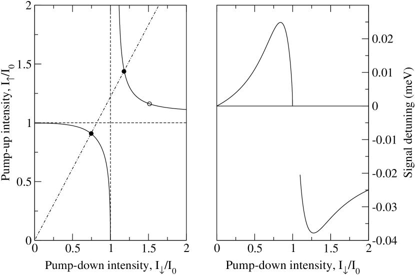
Figure 1: Left panel: allowed intensities of the pump fields giving steady-state operation with $g=0.2$(solid lines), and $g=0$(dashed lines). The sloping line and dots are for comparison with Fig. 4. The sloping line is a circularity of $\sigma=0.1$ for the pump fields, corresponding to the circularity of the drive used for Fig. 4. The dots mark the pump fields at the thresholds of Fig. 4. Right panel: corresponding signal detuning for $g=0.2$. For both plots $\gamma_{s}=0.25{\mathrm{meV}}$,$\gamma_{i}=1.0{\mathrm{meV}}$, $\mbox{$|\mbox{\scriptsize{\it X}}_{s}|$}^{2}=0.5,\mbox{$|\mbox{\scriptsize{\it X}}_{i}|$}^{2}=0.97$, and $\delta_{p}=0$. The intensities of the pump fields are given relative to that for steady-state operation with a single polarisation, $I_{0}$.

In Fig.1, we illustrate the pump fields and signal detunings giving steady-state operation, for a resonant pump with $\mbox{$\gamma_{s}$}=0.25{\mathrm{meV}}$, $\mbox{$\gamma_{i}$}=1{\mathrm{meV}}$, $g=0.2$, and the Hopfield coefficients $\mbox{$|\mbox{\scriptsize{\it X}}_{s}|$}^{2}=0.5$ and $\mbox{$|\mbox{\scriptsize{\it X}}_{i}|$}^{2}=0.97$. We have estimated these damping rates and Hopfield coefficients to be those of the experiment reported in Ref. lagoudakis2002, . The curves describing the allowed pump fields look very similar to those for the uncoupled device, shown as dashed lines, except that the degeneracy, where both polarisations are on threshold, has been split. The signal detuning shows small deviations from the uncoupled case, where it would be zero with this resonant pump. These shifts of the signal detuning from its uncoupled value are due to the spin-flip processes and the imbalance in the damping of the signal and idler; without spin-flips or for $\mbox{$\gamma_{s}$}^{\prime}=\mbox{$\gamma_{i}$}^{\prime}$ the condition for the intensities to be real is $\Im\mbox{$\Delta_{s}$}\mbox{$\Delta_{i}^{*}$}=0$, as in the uncoupled device.

We can determine whether the form shown in Fig 1 is general for small $g$ by using perturbation theory to calculate how the degeneracy is split by the coupling. We expand the left-hand side of Eq. 7 to first-order in the deviation of the pump intensities from the degeneracy and the change in the detunings compared to the uncoupled case, and take the right-hand side to be unchanged to leading order. Eliminating the detunings such that the fields remain real, we find that the shifts in the pump intensities obey a real quartic form. Owing to its complexity, we have not studied this quartic in general. However, for the special case of a resonant pump it becomes

$$4I_{0}^{2}(a^{\prime}-4I_{0}^{2}\delta I_{\uparrow})(\delta I_{\uparrow}+\delta I_{\downarrow})^{2}+a^{\prime\prime^{2}}=0,$$ (8)

where $a=a^{\prime}+ia^{\prime\prime}$ is the right-hand side of Eq. 7 evaluated on the degeneracy. Eq. 8 always has the form seen near the degeneracy in Fig. 1, so the structure of that figure is general for resonant pumping and small $g$.

We can also use perturbation theory away from the degeneracy, to study the shift in the allowed pump fields produced by a small $g$. Again for a resonant pump, the leading deviation in $I_{\uparrow}$ from an uncoupled solution in which $I_{\uparrow}=I_{0}$ is on threshold while $I_{\downarrow}$ is well away from it obeys

$$\delta I_{\uparrow}=-\frac{g^{2}I_{\downarrow}}{2(\mbox{$\gamma_{s}$}^{\prime}\mbox{$\gamma_{i}$}^{\prime}-I_{\downarrow}^{2})}\left(4I_{\downarrow}\sqrt{\mbox{$\gamma_{s}$}^{\prime}\mbox{$\gamma_{i}$}^{\prime}}-(\mbox{$\gamma_{s}$}^{\prime}-\mbox{$\gamma_{i}$}^{\prime})^{2}\right).$$

Thus for a small value of one polarisation, turning on the cross-polarisation coupling increases the threshold for the other polarisation. There is therefore a region of $I_{\downarrow}$, just above the uncoupled threshold, in which $I_{\uparrow}(I_{\downarrow})$ is multivalued, although this is not visible on the scale of Fig. 1. Such behaviour is possible because in the uncoupled device the signal and idler fields of the below-threshold polarisation are zero, and hence there is no loss through these channels. With a finite coupling however, these fields become finite, providing another loss channel. The modes do not always mix in this way however; for general pump detunings the initial shift can be to higher or lower thresholds.

In the strong-coupling limit, $g\to\infty$, the solutions to Equation 7 for $\gamma_{s}^{\prime}\neq\gamma_{i}^{\prime}$ have either $I_{\uparrow}$ or $I_{\downarrow}=0$. The approach to this limit is illustrated in Fig.2, where we plot the allowed pump fields for increasing values of $g$. The lower branch simply collapses towards the origin. The upper branch disappears, then reappears as two disjoint branches with asymptotes $I_{\uparrow}=0$ and $I_{\downarrow}=0$. These branches then merge, before finally collapsing into the origin.

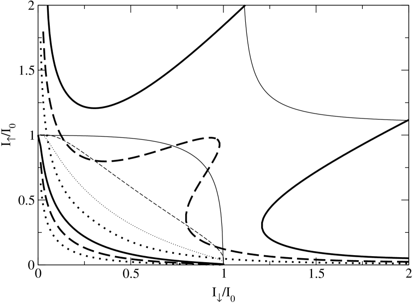
Figure 2: Allowed pump-up intensity as a function of pump-down intensity for $g=0.2$(thin solid lines), 1.0(thin dashed line), 2.0(thin dotted line), 5.0(thick solid lines), 7.0(thick dashed lines), 10.0(thick dotted lines). The remaining parameters are as used for figure 1.

III.2 Signal and idler fields

We now consider the signal and idler fields in the steady-states. These fields are determined, up to an overall complex scale factor $z$, by the eigenvector of $M$ corresponding to the zero eigenvalue.

The eigenvectors of $M$, unlike the eigenvalues, depend on the phases of the pump fields, $\phi_{\uparrow}$ and $\phi_{\downarrow}$. This dependence can be extracted by noting that $M$ can be written in the form $S^{\dagger}MS$, where $S$ is a diagonal matrix with entries $e^{-i\phi_{\uparrow}},e^{i\phi_{\uparrow}},e^{-i\phi_{\downarrow}},e^{i\phi_{\downarrow}}$. Thus the phases of the pump fields simply shift the arguments of the steady-state signal and idler fields: supposing $\vec{e}=(\mbox{$s_{\uparrow}$},\mbox{$i_{\uparrow}^{*}$},\mbox{$s_{\downarrow}$},\mbox{$i_{\downarrow}^{*}$})$ is an eigenvector of $M$ when $\phi_{\uparrow}=\phi_{\downarrow}=0$, then $\vec{e^{\prime}}=(\mbox{$s_{\uparrow}$}e^{i\phi_{\uparrow}},\mbox{$i_{\uparrow}^{*}$}e^{-i\phi_{\uparrow}},\mbox{$s_{\downarrow}$}e^{i\phi_{\downarrow}},\mbox{$i_{\downarrow}^{*}$}e^{-i\phi_{\downarrow}})$ is the corresponding eigenvector for finite phases. The phases of the pump fields have such a simple effect because there is no phase dependence in the form of the interaction energy we have chosen. A nonlinearity such as $(\Re\phi)^{4}$, rather than $|\phi|^{4}$, might lead to a more complicated effect of the pump phases.

In Fig. 3, we plot the components of the eigenvector of zero eigenvalue for the pump fields shown in Fig. 1. We have normalised the eigenvector so that the total intensity is one and the phase of the signal up field is zero, and taken the pump fields to be real and positive. The idler fields are always smaller than the corresponding signal fields due to the stronger damping of the idlers. The crossings of the signal curves occur when the intensities in the two pump components are equal. In the region $I_{\downarrow}/I_{0}<1$, the polarisation with the largest pump fields also has the largest signal and idler fields, but that ordering is reversed in the region $I_{\downarrow}/I_{0}>1$. For $I_{\downarrow}/I_{0}<1$, the phase differences between corresponding components in the two polarisations lie near to zero, while for $I_{\downarrow}/I_{0}>1$ they lie near to $\pi$.

The two circular components of the signal field can be combined to form, in general, an elliptically polarised state. The phase differences between the two components of the signal that can be seen in Fig.3 correspond to rotations of the ellipse describing the signal polarisation compared with that describing the pump polarisation. Such polarisation rotations are absent in our model if there are no spin-flip processes.

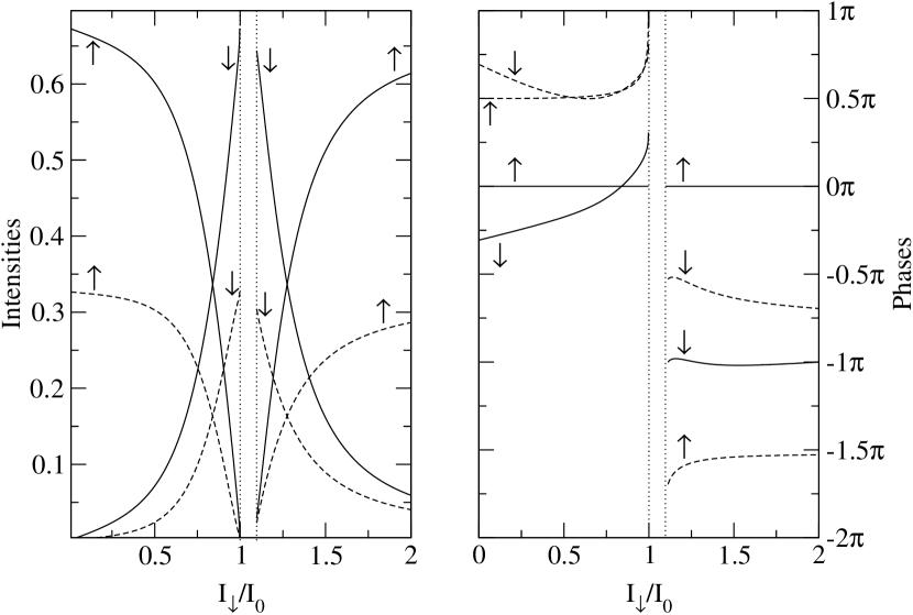
Figure 3: Signal fields(solid lines) and conjugate of the idler fields(dashed lines) corresponding to the steady-states shown in Fig. 1, scaled such that the total intensity is one and the phase of the signal up component is zero.

III.3 Dependence on the driving fields

The steady-state reached in the device is selected from the possibilities shown in Fig. 1 by the external driving fields, according to the steady-state version of the pump equation (2a)

$$\mbox{$\Delta_{p}$}\mbox{$p_{\uparrow}$}+2\mbox{$s_{\uparrow}$}\mbox{$i_{\uparrow}$}\mbox{$p_{\uparrow}^{*}$}+\mbox{$g$}(\mbox{$s_{\downarrow}$}\mbox{$i_{\uparrow}$}+\mbox{$s_{\uparrow}$}\mbox{$i_{\downarrow}$})\mbox{$p_{\downarrow}^{*}$}$$ (9)

$$+\mbox{$g$}(\mbox{$s_{\uparrow}$}\mbox{$s_{\downarrow}^{*}$}+\mbox{$i_{\uparrow}$}\mbox{$i_{\downarrow}^{*}$})\mbox{$p_{\downarrow}$}=F_{\uparrow},$$

and its spin flipped counterpart. The first term on the left-hand side of Eq. 9 describes the bare response of the pump field, while the remaining “pump depletion” terms describe the effect on the pump fields of the nonlinear processes which generate the signal and idler. The pump equations (9) determine the remaining four real unknowns: $I_{\downarrow}$, the arguments of the pump fields, and the total intensity of the output fields, $|z|^{2}$. The pump equations are independent of the overall phase of the zero eigenvector, $\arg z$, corresponding to a single free phase among the output fields.

To solve the pump equations (9), we first extract the dependence of the phases of the signal and idler on the phases of the pump, as discussed in section III.2. This gives

$$e^{i\arg p_{\uparrow}}\left|L_{\uparrow}\right|=|F_{\uparrow}|e^{i\arg F_{\uparrow}},$$ (10)

where $L_{\uparrow}$ is the left-hand side of Eq. 9 evaluated for $\arg p_{\uparrow}=0$. Taking the modulus of Eq. 10 we have the general form

$$|\alpha+|z|^{2}\beta|=|F_{\uparrow}|,$$ (11)

where $\alpha$ and $\beta$ are functions of the intensities of the pump fields. We solve Eq. 11 to determine the output intensities that are consistent with the strength of the pump-up driving, as functions of the intensities of the pump fields $I_{\uparrow}(I_{\downarrow})$ and $I_{\downarrow}$. We then solve the spin-flipped version of Eq. 11 to determine the output intensities consistent with the strength of the pump-down driving. Equating these two intensities gives a nonlinear equation which we solve to determine $I_{\downarrow}$ as a function of the external pumps.

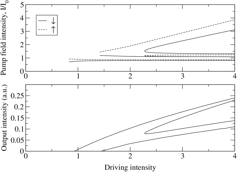
Figure 4: Steady-states, for the parameters of Fig. 1, with an external drive of circularity $\sigma=0.1$ and varying intensity. The intensity of the drive is expressed relative to that of the lowest threshold in the uncoupled device with the same parameters.

Fig.4 illustrates the solution to the pump equations (9). The damping and Hopfield coefficients for the signal and idler are as in Fig.1. For the pump we have used $\gamma_{p}=0.1{\mathrm{meV}}$ and $\mbox{$|\mbox{\scriptsize{\it X}}_{p}|$}^{2}=0.8$, which we again estimate to be appropriate to the system reported in Ref.  lagoudakis2002, . We have taken an external drive of fixed circularity, $\sigma=0.1$, and varying intensity. The top panel shows the intensities of the pump fields, and the bottom panel shows the output intensity. Increasing the driving intensity from zero we first find two continuous thresholds, where steady-states appear starting with zero output intensity. The pump fields at these thresholds are marked as filled dots on Fig.1. At these points, the pump intensities match, up to a common factor, with the driving intensities: $I_{\uparrow\downarrow}=|F_{\uparrow\downarrow}|^{2}/|\mbox{$\Delta_{p}$}|^{2}$. For this small value of $g$, they are approximately the thresholds for each polarisation of the uncoupled device. With increasing driving, the output intensity in each of these steady-states increases and, in constrast to the uncoupled device, the pump fields change. Increasing the driving intensity still further, we find a third threshold at which a new steady-state appears, and then splits into two states. This third threshold is discontinuous, i.e. the solution appears with a finite output intensity. It corresponds to the pump fields marked with the open dot on Fig. 1.

IV Discussion

In Ref. tartakovskii2000, , the intensity and circularity of the signal output was measured under continuous driving of the pump field. The driving circularity was varied from circular to linear and the total pump intensity was of the same order of magnitude as the threshold for a circularly polarised pump. As the pump circularity $\sigma$ was decreased from one, the signal intensity increased by a factor of five to a maximum at $\sigma\approx 0.4$, and then decreased again. The circularity of the signal was approximately constant, except near to linear pumping, where it dropped to zero.

Considering the pair process underlying the parametric oscillator, one might expect that without polarisation coupling the output would monotonically reduce as the pump circularity is reduced: scattering only occurs within each polarisation, and moving away from circularity reduces the population of each polarisationlagoudakis2002 . However, such an interpretation overlooks the effects of pump depletion and coherence. Because of these effects, the steady-state output of a single polarisation pumped with intensity $I_{+}$ is actually proportional to $\sqrt{I_{+}}-\sqrt{I_{\mathrm{thresh}}}$(Ref. whittaker2001, ). For total driving intensities greater than twice the single-polarisation threshold, there is a critical pump circularity below which both polarisations are above threshold. Below this critical circularity, the total output increases as the pump circularity is reduced, with a local maximum for a linear pump. Thus an increase in the output as the pump circularity is reduced does not in general imply the existence of polarisation coupling. However, without such a coupling it is difficult to explain the dependence of output on pump circularity reported in Ref. tartakovskii2000, : the enhancement away from circularity is too strong, and the output peaks for elliptical, rather than circular or linear, pumping.

The lower branches shown on Fig.2 have no structure to suggest that they would give a maximum output for an elliptically polarised pump. However, the upper branches illustrated for $g=5$ and $g=7$ do have such structure. As the pump circularity is reduced from one, we would first go up through the threshold for these solutions, then move back towards it, and for some parameters go below it again as we approach linear pumping. The circularity of the turning points illustrated for $g=7$ is $\sigma=0.47$. While this is roughly consistent with the experimental results, a detailed fit to the experiment is beyond the scope of the present paper. It would involve a large number of parameters, and we expect the results to be sensitive to details left out of the present model such as the blueshifts.

It is only stable steady-states which are relevant to continuously pumped experiments. We have analysed the stability of some of the steady-state solutions to our model for a special case in which all the effective damping rates are equal, $\gamma_{p}^{\prime}=\gamma_{s}^{\prime}=\gamma_{i}^{\prime}$. For $g=0.1$, there are two solutions with continuous thresholds and two with discontinuous thresholds, as there are in Fig. 4. We find that only the solution with the lowest threshold is stable. For $g=2.0$, we find only one solution with a continuous threshold, as well as two with discontinuous thresholds. In that case, both the continuous solution and one of the discontinuous solutions is stable. Thus it is possible for our model to have stable solutions other than that with the lowest threshold, and to have more than one stable solution.

The pulsed experiments of Ref. lagoudakis2002, have recently been addressed by Kavokin et al. kavokin2003 . Their theory reproduces the experimentally observed rotations of the linear polarisation without scattering between polarisations. In their theory, the rotation of the linear polarisation comes from the different blueshifts of the two circular polarisation states. The present work does not include this effect, because we have taken the detunings of the two polarisation states to be the same. We expect that if the blueshifts are small compared with the interactions between polarisations then the steady-states will only contain a single frequency for the pump, signal and idler, and the treatment given here will be qualitatively correct. However, a splitting of the two circular polarisation states might be an alternative explanation for the steady-states results of Ref. tartakovskii2000, .

The agreement between the polarisation rotations seen in the pulsed experimentslagoudakis2002 and the theory of Ref. kavokin2003, suggests that a polarisation coupling term is not required to explain these results. However, this does not imply that the polarisation coupling is always irrelevant. The polarisation rotations produced by a coupling could be small compared with those produced by the blueshifts, allowing a good fit to this aspect of the data without a coupling. Note also that the pulsed experiments are done at much higher excitation powers, typically around a hundred times greater, than the steady-state experiments. The polarisation coupling could also depend on sample parameters such as the energy difference between the pump polaritons and the biexcitontartakovskii2000 .

An interaction of the form we propose corresponds microscopically to an interaction between excitons of opposite spin, which could come from the Coulomb interactions between the electrons and the holes in the excitons. To first order in these Coulomb interactions, the interaction between opposite spin excitons is negligibleciuti1998 ; maialle1994 , because in that approximation small wavevector scattering is dominated by electron-electron and hole-hole exchange. Thus a finite value of $g$ implies the significance of higher-order processes, which can produce interactions between opposite spin excitonsmaialle1994 . We suggest that the higher-order processes could involve the $m_{j}=\pm 2$ excitons, which are close in energy, and produce an interaction at second order. Another recent suggestioninoue2000 is that the interaction involves excited states of the excitons.

V Conclusions

We have studied the steady-states of a model of microcavity parametric oscillation with coupled polarisations. For small values of the coupling, we find two steady-states corresponding to those of the uncoupled device. However, due to the increased scope for arranging the pump depletion, there are also two steady-states which appear discontinuously, i.e. with a finite value of the output intensity, as the driving intensity is increased. For general values of the coupling Fig.2 suggests that there will be either one or two continuous solutions, depending on the coupling and pump circularity. There may also be discontinuous solutions. For some parameters more than one steady-state can be stable, in which case it should be possible to observe switching between the states induced either by noise or by external probes.

The coupling between polarisations introduces two types of mixing term into the equations of motion for the fields. As well as the straightforward analog of the process considered in the uncoupled model, there are processes which exchange the spins of two fields. Such spin-flip processes lead to a rotation of the output polarisation with respect to the pump. They also produce shifts in the output frequencies with varying pump intensity or circularity, even in the absence of the shifts associated with the mean-field exciton-exciton interaction.

- (1) For reviews of basic properties of microcavities, see M. S. Skolnick, T. A. Fisher and D. M. Whittaker, Semicond. Sci. Technol. 13, 645 (1998); G. Khitrova, H. M. Gibbs, F. Jahnke, M. Kira and S. W. Koch, Rev. Mod. Phys. 71, 1591 (1999).
- (2) P. G. Savvidis, J. J. Baumberg, R. M. Stevenson, M. S. Skolnick, D. M. Whittaker and J. S. Roberts, Phys. Rev. Lett. 84 1547 (2000).
- (3) J. Erland, V. Mizeikis, W. Langbein, J. R. Jensen and J. M. Hvam, Phys. Rev. Lett. 86, 5791 (2001).
- (4) R. M. Stevenson, V. N. Astratov, M. S. Skolnick, D. M. Whittaker, M. Emam-Ismail, A. I. Tartakovskii, P. G. Savvidis, J. J. Baumberg and J. S. Roberts, Phys. Rev. Lett. 85 3680 (2000).
- (5) See, for example, Y. R. Shen in The Principles of Nonlinear Optics (Wiley, 1984), Chapter 9.
- (6) C. Ciuti, P. Schwendimann, B. Deveaud and A. Quattropani, Phys. Rev. B62, R4825 (2000).
- (7) D. M. Whittaker, Phys. Rev. B63 193305 (2001).
- (8) C. Ciuti, P. Schwendimann and A. Quattropani, Phys. Rev. B63, 041303 (2001).
- (9) S. Savasta, O. Di Stefano, and R. Girlanda, Phys. Rev. Lett. 90 096403 (2003)
- (10) A. I. Tartakovskii, D. N. Krizhanovskii and V. D. Kulakovskii, Phys. Rev. B62 13298(R) (2000).
- (11) P. G. Lagoudakis, P. G. Savvidis, J. J. Baumberg, D. M. Whittaker, P. R. Eastham, M. S. Skolnick and J. S. Roberts Phys. Rev. B65 161310(R) (2002).
- (12) A. Kavokin, G. Malpuech, P. G. Lagoudakis, J. J. Baumberg, K. Kavokin, Phys. Stat. Sol. A 195 579 (2003).
- (13) M. Kuwata-Gonokami, S. Inouye, H. Suzuura, M. Shirane, R. Shimano, T. Someya, H. Sakaki, Phys. Rev. Lett. 79 1341 (1997).
- (14) K. Bott, O. Heller, D. Bennhardt, S. T. Cundiff, P. Thomas, E. J. Mayer, G. O. Smith, R. Eccleston, J. Kuhl, K. Ploog, Phys. Rev. B48 17418 (1993).
- (15) M. Z. Maialle and L. J. Sham, Phys. Rev. Lett. 73 3310 (1994).
- (16) C. Ciuti, V. Savona, C. Piermarocchi, A. Quattropani, and P. Schwendimann, Phys. Rev. B58 7926 (1998)
- (17) J. I. Inoue, T. Brandes and A. Shimizu, Phys. Rev. B61 2863 (2000).