Extended floor field CA model for evacuation dynamics

Abstract

The floor field model, which is a cellular automaton model for studying evacuation dynamics, is investigated and extended. A method for calculating the static floor field, which describes the shortest distance to an exit door, in an arbitrary geometry of rooms is presented. The wall potential and contraction effect at a wide exit are also proposed in order to obtain realistic behavior near corners and bottlenecks. These extensions are important for evacuation simulations, especially in the case of panics.

I Introduction

Recent progress in modelling pedestrian dynamics book is remarkable and many valuable results are obtained by using different models, such as the social force model HFV and the floor field model BKAJ ; AA . The former model is based on a system of coupled differential equations which has to be solved e.g. by using a molecular dynamics approach similar to the study of granular matter. Pedestrian interactions are modelled via long-ranged repulsive forces. In the latter model two kinds of floor fields, i.e., a static and a dynamic one, are introduced to translate a long-ranged spatial interaction into an attractive local interaction, but with memory, similar to the phenomenon of chemotaxis in biology chemo . It is interesting that, even though these two models employ different rules for pedestrian dynamics, they share many properties including lane formation, oscillations of the direction at bottlenecks BKAJ , and the so-called faster-is-slower effect HFV . Although these are important basics for pedestrian modelling, there are still many things to be done in order to apply the models to more practical situations such as evacuation from a building with complex geometry.

In this paper, we will propose a method to construct the static floor field for complex rooms of arbitrary geometry. The static floor field is an important ingredient of the model and has to be specified before the simulations. Moreover, the effect of walls and contraction at a wide exit will be taken into account which enables us to obtain realistic behavior in evacuation simulations even for the case of panic situations.

This paper is organized as follows. In Sec. II, we cite experimental data of evacuations to illustrate the strategy of people in panic situations. Then an extended floor field model is introduced in Sec. III including a method of constructing the floor field and wall potentials. In Sec. IV results of simulations for various configurations of a room are investigated and concluding discussions are given in Sec. V.

II Human behaviour in panic situations

First we discuss the different kinds of human behavior in panic situations. People in a room try to evacuate in case of fire with their own strategy. The strategies of the evacuation are well studied up to now, and we cite an example of an experiment of evacuation that was conducted in a large supermarket in Japan Abe . Fire alarms and false smoke were set suddenly in the experiment, and after people had escaped from the building they have been interviewed about their choice of escape routes etc. Data from more than 300 people were collected. The following list shows the statistics of the answers given:

1. I escaped according to the signs and instructions, and also broadcast or guide by shopgirls (46.7%).

2. I chose the opposite direction to the smoking area to escape from the fire as soon as possible (26.3%).

3. I used the door because it was the nearest one (16.7%).

4. I just followed the other persons (3.0%).

5. I avoided the direction where many other persons go (3.0%).

6. There was a big window near the door and you could see outside. It was the most “bright” door, so I used it (2.3%).

7. I chose the door which I’m used to (1.7%).

We see that very different, sometimes even contradictory, choices were made indicating the complexity of an evacuation problem. If we assume that there are no signs and no guidance by broadcasts as well as no information about the location of the fire, then according to the questionnaires, people will try to evacuate by relying on both one’s memory of the route to the nearest door and other people’s behavior. This competition between collective and individual behavior is essential for modelling evacuation phenomena. It is included in the static and dynamic floor fields of our model that we have introduced in previous papers BKAJ ; AA ; AKA .

III An extended floor field model

In this section we will summarize the update rules of an extended floor field model for modelling panic behavior of people evacuating from a room. The space is discretized into cells of size $40\,{\rm cm}\times 40\,{\rm cm}$ which can either be empty or occupied by one pedestrian (hard-core-exclusion). Each pedestrian can move to one of the unoccupied next-neighbor cells $(i,j)$ (or stay at the present cell) at each discrete time step $t\to t+1$ according to certain transition probabilities $p_{ij}$ (Fig. 1) as explained below in Sec. III.1.

For the case of evacuation processes, the static floor field $S$ describes the shortest distance to an exit door. The field strength $S_{ij}$ is set inversely proportional to the distance from the door. The dynamic floor field $D$ is a virtual trace left by the pedestrians similar to the pheromone in chemotaxis chemo . It has its own dynamics, namely diffusion and decay, which leads to broadening, dilution and finally vanishing of the trace. At $t=0$ for all sites $(i,j)$ of the lattice the dynamic field is zero, i.e., $D_{ij}=0$. Whenever a particle jumps from site $(i,j)$ to one of the neighboring cells, $D$ at the origin cell is increased by one.

The model is able to reproduce various fundamental phenomena, such as lane formation in a corridor, herding and oscillation at a bottleneck BKAJ ; AA . This is an indispensable property for any reliable model of pedestrian dynamics, especially for discussing safety issues.

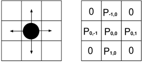
Figure 1: Target cells for a person at the next time step. The von Neumann neighborhood is used for this model.

III.1 Basic update rules

The update rules of our CA have the following structure:

1. The dynamic floor field $D$ is modified according to its diffusion and decay rules, controlled by the parameters $\alpha$ and $\delta$. In each time step of the simulation each single boson of the whole dynamic field $D$ decays with probability $\delta$ and diffuses with probability $\alpha$ to one of its neighboring cells.

2. For each pedestrian, the transition probabilities $p_{ij}$ for a move to an unoccupied neighbor cell $(i,j)$ are determined by the two floor fields and one’s inertia (Fig. 1). The values of the fields $D$ (dynamic) and $S$ (static) are weighted with two sensitivity parameters $k_{D}$ and $k_{S}$:

   $$p_{ij}=N\exp{\left(k_{D}D_{ij}\right)}\exp{\left(k_{S}S_{ij}\right)}p_{I}(i,j)p_{W},$$ (1)

   with the normalization $N$. Here $p_{I}$ represents the inertia effect BKAJ given by $p_{I}(i,j)=\exp{\left(k_{I}\right)}$ for the direction of one’s motion in the previous time step, and $p_{I}(i,j)=1$ for other cells, where $k_{I}$ is the sensitivity parameter. $p_{W}$, newly introduced in this paper, is the wall potential which is explained below. In (1) we do not take into account the obstacle cells (walls etc.) as well as occupied cells.

3. Each pedestrian chooses randomly a target cell based on the transition probabilities $p_{ij}$ determined by (1).

4. Whenever two or more pedestrians attempt to move to the same target cell, the movement of all involved particles is denied with probability $\mu\in[0,1]$, i.e. all pedestrians remain at their site AKA . This means that with probability $1-\mu$ one of the individuals moves to the desired cell. Which one is allowed to move is decided using a probabilistic method BKAJ ; AKA .

5. The pedestrians who are allowed to move perform their motion to the target cell chosen in step 3. $D$ at the origin cell $(i,j)$ of each moving particle is increased by one: $D_{ij}\to D_{ij}+1$, i.e. $D$ can take any non-negative integer value.

The above rules are applied to all pedestrians at the same time (parallel update). Some important details are explained in the following subsections.

III.2 Effect of walls

People tend to avoid walking close to walls and obstacles. This can be taken into account by using “wall potentials”. We introduce a repulsive potential inversely proportional to the distance from the walls. The effect of the static floor field is then modified by a factor (see eq. (1)):

$$p_{W}=\exp(k_{W}\min(D_{\rm max},d)),$$ (2)

where $d$ is the minimum distance from all the walls, and $k_{W}$ is a sensitivity parameter. The range of the wall effect is restricted up to the distance $D_{\rm max}$ from the walls.

Fig. 2 shows an example for an evacuation from a room with obstacles using the wall potential. Without wall potentials ($k_{W}=0$), jamming areas near every corner can be observed, because everybody tries to evacuate along the same path of minimum length. For $k_{W}\neq 0$ these areas are clearly suppressed. Thus the introduction of this additional potential improves the realism of the model.

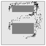
(a)                          (b)

Figure 2: Snapshot of evacuation (a) without ($k_{W}=0$) and (b) with ($k_{W}=0.5$) wall potential. We can clearly see the artifact of jamming at every corner without the wall potential. Parameters are $D_{\rm max}=10,k_{S}=2.0,k_{D}=1.0,k_{I}=0.2,\mu=0.2$ and the initial density is $\rho=0.03$.

III.3 Calculation of the static field in arbitrary geometries

(a)

(b)

Figure 3: Example for the calculation of the static floor field using the Dijkstra method. (a) A room with one obstacle. The door is at $O$ and the obstacle is represented by lines $A-H$. (b) The visibility graph for this room. Each node connected by a bond is “visible”, i.e., there are no obstacles between them. The real number on each bond represents the distance between them as an illustration.

In the following we propose a combination of the visibility graph and Dijkstra’s algorithm to calculate the static floor field. These methods enable us to determine the minimum Euclidian ($L^{2}$) distance of any cell to a door with arbitrary obstacles between them.

Let us explain the main idea of this method by using the configuration given in Fig. 3(a) where there is an obstacle in the middle of the room. We will calculate the minimum distance between a cell $P$ and the door $O$ by avoiding the obstacle. If the line $PO$ does not cross the obstacle $A-H$, then the length of the line, of course, gives the minimum. If, however, as in the example given in Fig. 3(a), the line $PO$ crosses the obstacle, one has to make a detour around it. Then we obtain two candidates for the minimum distance, i.e., lines $PBAO$ and $PCDHO$. The shorter one finally gives the minimum distance between $P$ and $O$. If there are more than one obstacle in the room, then we apply the same procedure to each of them repeatedly. Here it is important to note that all the lines pass only the obstacle’s edges with an acute angle. It is apparent that the obtuse edges like $E$ and $F$ can never be passed by the minimum lines.

To incorporate this idea into the computer program, we first need the concept of the visibility graph in which only the nodes that are visible to each other are bonded CG (“visible” means here that there are no obstacles between them). The set of nodes consists of a cell point $P$, a door $O$ and all the acute edges in the room. In the case of Fig. 3(a), the node set is $\{P,O,A,B,C,D,G,H\}$ and the bonds are connected between $A-B$, $A-H$, and so on (Fig. 3(b)). Each bond has its own weight which corresponds to the Euclidian distance between them.

Once we have the visibility graph, we can calculate the distance between $P$ and $O$ by tracing and adding the weight of the bonds between them. There are several possible paths between $P$ and $O$, and the one with minimum total weight represents the shortest route between them. The optimization task is easily performed by using the Dijkstra method CG which enables us to obtain the minimum path on a weighted graph.

Performing this procedure for each cell in the room, the method allows us to determine the static floor field for arbitrary geometries. We will call this metric Dijkstra metric in the following. Results for a complex static floor field obtained by this method are shown in Fig. 4. There are two doors in this room, thus we calculate the minimum distance for each door from each cell in the room and take the shorter one as value of the static floor field.

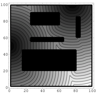
Figure 4: A contour plot of the static floor field by using the Dijkstra metric. There are four obstacles and two doors in this room. The darkness of shading is inversely proportional to the distance from the nearest door.

Next, we like to point out the advantages of the Dijkstra metric compared to the simpler Manhattan metric AA . Fig. 5 shows a comparison of typical configurations during an evacuation from a simple room with no obstacles by using both the Dijkstra and the Manhattan metric. We see that for large $k_{S}$ the pedestrians move preferably along a line in front of the door if the Manhattan metric is used, whereas for the Dijkstra metric the behavior is more realistic.

(a)                          (b)

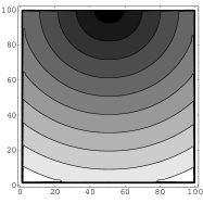
(c)                          (d)

Figure 5: Comparison of typical snapshots in the case of the Manhattan (a) and Dijkstra (c) metric for the static floor field. We see an artifact of line formation in front of the door in (a). This comes from the nonisotropic nature of the Manhattan metric as seen in the contour plot (b), while the Dijkstra metric gives an isotropic static floor field from the door (d). Parameters are $k_{S}=3.0,k_{D}=1.0,k_{I}=0.2,\mu=0.2$ and the initial density is $\rho=0.04$.

III.4 Diffusion and decay of the dynamical floor field

We can show that the order of diffusion and decay process in rule 1 (see Sec. III.1) is exchangeable, i.e., it makes no difference no matter which of the two processes is applied first. Both diffusion process and decay can be written in difference form as

$$D^{t+1}_{ij} = D^{t}_{ij}-\alpha D^{t}_{ij}$$ (3)

$$+ \frac{\alpha}{4}(D^{t}_{i+1,j}+D^{t}_{i-1,j}+D^{t}_{i,j+1}+D^{t}_{i,j-1}),$$

$$D^{t+1}_{ij} = D^{t}_{ij}-\delta D^{t}_{ij},$$ (4)

respectively. Thus the combination of the diffusion and decay above gives

$$D^{t+1}_{ij} = (1-\alpha)(1-\delta)D^{t}_{ij}+\frac{\alpha(1-\delta)}{4}(D^{t}_{i+1,j}$$

$$+ +D^{t}_{i-1,j}+D^{t}_{i,j+1}+D^{t}_{i,j-1})$$ (5)

regardless of their order.

In BKAJ also a continuous dynamic floor field has been investigated. It was observed that this has no qualitative influence on the behavior of the model. This comes from the fact that the continuum limit of (5) is the same as the continuous version in BKAJ . The limit of (5) is given by

$$\frac{\partial D}{\partial t}=-d_{1}D+\frac{\alpha d_{2}}{4}\left(\frac{\partial^{2}D}{\partial x^{2}}+\frac{\partial^{2}D}{\partial y^{2}}\right),$$ (6)

where $\delta/\Delta t=d_{1}$ and $(\Delta x)^{2}/\Delta t=(\Delta y)^{2}/\Delta t=d_{2}$ (time and space intervals are written as $\Delta t$ and $\Delta x$, $\Delta y$), respectively, and $d_{1},d_{2}$ and $\alpha$ are kept constant in the limit $\Delta x,\Delta y,\Delta t,\delta\to 0$. Therefore the dynamics of $D$ given by (6) coincides with the previous one if we choose appropriate coefficients.

III.5 Model parameters and their physical relevance

There are several parameters in our model, and the most important ones are listed below with their physical meaning which is helpful in understanding the collective behavior in the simulations.

1. $k_{S}\in[0,\infty[\cdots$ The coupling to the static field characterizes the knowledge of the shortest path to the doors, or the tendency to minimize the costs due to deviation from a planned route Ho . This considerably controls one’s velocity and evacuation times.

2. $k_{D}\in[0,\infty[\cdots$ The coupling to the dynamic field characterizes the tendency to follow other people (herding behavior). The ratio $k_{D}/k_{S}$ may be interpreted as the degree of panic. It is known that people try to follow others particulary in panic situations HFV (see Sec. II). This tendency lasts at least until they can escape without any hindrance. If hindrance by other people takes place often and a tendency to clogging emerges, people try to avoid such directions. This is taken into account in our dynamic floor field which is proportional to the velocity density, such that people will follow only moving persons.

3. $k_{I}\in[0,\infty[\cdots$ This parameter determines the strength of inertia which suppresses quick changes of the direction of motion. It also reflects the tendency to minimize the costs due to deviation from one’s desired route and acceleration Ho .

4. $\mu\in[0,1]\cdots$ The friction parameter controls the resolution of conflicts in clogging situations. Both cooperative and competitive behavior at a bottleneck are well described by adjusting $\mu$ AHKAM .

5. $\alpha,\delta\in[0,1]\cdots$ These constants control diffusion and decay of the dynamic floor field. It reflects the randomness of people’s movement and the visible range of a person, respectively. If the room is full of smoke, then $\delta$ takes large value due to the reduced visibility. Through diffusion and decay the trace is broadened, dilute and vanishes after some time.

6. $k_{W},D_{\rm max}\cdots$ These parameters specify the wall potential. Pedestrians tend to avoid walking close to walls and obstacles. $D_{\rm max}$ is the maximum distance at which people feel the walls. It reflects one’s range of sight or so-called personal space space . $k_{W}$ is the sensitivity to the walls, and the ratio $k_{W}/k_{S}$ reflects to which degree deviations from the shortest route (which is determined by the static floor field) are accepted to avoid the walls.

IV Simulations

We focus on measuring the total evacuation time by changing the parameters $k_{S},k_{D},k_{I},\mu$ and the configuration of the room, such as width, position and number of doors and obstacles. In all simulations we put $D_{\rm max}=10$, $\alpha=0.2$ and $\delta=0.2$, and von Neumann neighborhoods are used in eq. (1) for simplicity. The size of the room is set to 100 $\times$ 100 cells.

In the previous papers BKAJ ; AA ; AKA , the influence of the two floor fields on the total evacuation time has been studied in detail. Here, the effects of inertia and wall potentials are investigated for concave rooms with some obstacles by using the Dijkstra metric.

IV.1 Inertia effect

Pedestrians try to keep their preferred velocity and direction as long as possible. This is taken into account by adjusting the parameter $k_{I}$. In Fig. 6, total evacuation times from a room without any obstacles are shown as function of $k_{D}$ in the cases $k_{I}=0$ and $k_{I}=3$. We see that it is monotonously increasing in the case $k_{I}=0$, because any perturbation from other people becomes large if $k_{D}$ increases, which causes the deviation from the minimum route. Introduction of inertia effects, however, changes this property qualitatively as seen in Fig. 6. The minimum time appears around $k_{D}=1$ in the case $k_{I}=3$. This is well explained by taking into account the physical meanings of $k_{I}$ and $k_{D}$. If $k_{I}$ becomes large, people become less flexible and all of them try to keep their own minimum route to the exit according to the static floor field regardless of congestion. By increasing $k_{D}$, one begins to feel the disturbance from other people through the dynamic floor field. This perturbation makes one flexible and hence contributes to avoid congestion. Large $k_{D}$ again works as strong perturbation as in the case of $k_{I}=0$, which diverts people from the shortest route largely. Thus we have the minimum time at a certain magnitude of $k_{D}$, which will depend on the value of $k_{S}$ and $k_{I}$.

Figure 6: Total evacuation time versus coupling $k_{D}$ to the dynamic floor field in the dependence of $k_{I}$. The room is a simple square without obstacles and 50 simulations are averaged for each data point. Parameters are $\rho=0.03,k_{S}=2,k_{W}=0.3$ and $\mu=0$.

IV.2 Contraction at a wide exit

If the width of an exit becomes large, a more careful treatment is needed in the calculation of the static floor field. People tend to rush to the center of the exit to avoid the walls. Thus one should introduce an effective width of the exit by neglecting certain cells from its each end. We call this effect contraction in this paper, due to its similarity with the contraction effect in hydrodynamics where fluid runs through a orifice with a smaller diameter than that of the orifice immediately after the fluid goes out of it fluid . The shortest distance from a cell in the room to one of the exit cells is calculated by using the Dijkstra metric, but only those exit cells near the center of the door are taken into account owing to the contraction. Then we take the minimum of those shortest distances and use it as the value of the static floor field at the cell. Here we define the ratio of contraction of an exit as $c=W^{\prime}/W$, where $W$ is the true width of the exit and $W^{\prime}$ is the effective width. If $c=1$, i.e., there is no contraction, and we see the artifact of two crowds near the edges of the exit (Fig. 7(a)). Introducing the contraction makes the evacuation behavior more realistic (Fig. 7(b)).

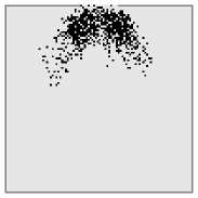
(a)                          (b)

Figure 7: Contraction of flow through a wide exit. The width of the exit is set as 20 cells. In (a) we set the ratio of contraction as 1, while in (b) it is 0.3. In (a) we see the artifact of the crowd at both ends of the exit even if they can easily evacuate through the center of the exit. Parameters are $\rho=0.05,k_{I}=1.0,k_{S}=2.0,k_{D}=1.0,k_{W}=0.3$ and $\mu=0.2$.

IV.3 Effect of obstacles

Let us investigate the effect of the position of obstacles to the total evacuation time. In Fig. 8, we set up two rooms such that the total area of obstacles in both rooms is the same. However, it is important to notice that the maximum length to the exit is different for these rooms. The maximum length in room (b) is 124.6, which is longer than that in (a) (115.5). This difference affects the static floor field and hence the dynamics of people. The average total evacuation time in case (a) is given by 357.48 time steps, while in (b) it is 379.22 time steps. This implies that, even though the area of obstacles is the same, their positions in the room will affect the evacuation dynamics considerably through the static floor field. It is worth mentioning that this simulation is different from the column problem we have studied previously AKA . The existence of a small column in front of an exit does not change the static floor field so much, but works as a simple obstacle which divides the flow of evacuating people.

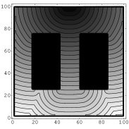
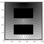
(a)                          (b)

Figure 8: The static floor field of rooms with same obstacles arranged in a different way. Although the total area of obstacles is the same, the maximum length to the exit in the room (a) is 115.5, while 124.6 in (b). Simulations are done with parameters $k_{S}=2.0,k_{D}=1.0,k_{I}=3.0,k_{W}=0.3,\mu=0.2$ and the initial density of the room is $\rho=0.03$.

IV.4 Influence of exit width and number of doors

Finally we study the effect of the width of an exit as well as the total number of doors in a room. We compare a room with an exit of size 10 to one with two exits of size 5 (Fig. 9). Although the total width of the exits is the same, the evacuation dynamics is different. The total evacuation time is 275 time steps in average for the case of one exit, but 245 for two exits (Fig.9(a)). If the two doors are set at opposite walls, the evacuation time is further improved to 220 time steps (Fig.9(b)). This is similar to the effect studied in Sec. IV.3, because the minimum length in the case of Fig. 9 (b) becomes 68.2 while it is 104.1 in (a).

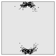
(a)                          (b)

Figure 9: A snapshot of an evacuation from a room with two exits. The total width of the exits is the same as for the one exit case. Simulations are done with parameters $k_{S}=2.0,k_{D}=1.0,k_{I}=1.0,k_{W}=0.3,\mu=0.2$ and $\rho=0.03$.

V Concluding discussion

In this paper we have discussed the main properties of the floor field cellular automaton model for pedestrian dynamics. A method for the calculation of the static floor field and the introduction of wall potentials has been proposed. Both extensions improve the realism of evacuation simulations. Also it is important to take into account the contraction in the case of wide exits. The existence of a minimal evacuation time in the case of finite inertia $k_{I}\neq 0$ is found, which shows the importance of one’s flexibility to respond to the other people’s behavior in the case of an evacuation. Finally it is shown that the position of obstacles in a room will affect the evacuation dynamics through the static floor field. Thus in architectural planning it is important to consider a suitable position of obstacles in a room as well as the exits carefully.

References

- (1) M. Scheckenberg and S.D. Sharma (Eds.), “Pedestrian and Evacuation Dynamics,” Springer-Verlag, Berlin, 2001.
- (2) D. Helbing, I. Farkas, and T. Vicsek, “Simulating dynamical features of escape panic,” Nature, vol.407, pp.487–490, 2000.
- (3) C. Burstedde, K. Klauck, A. Schadschneider, and J. Zittartz, “Simulation of pedestrian dynamics using a two-dimensional cellular automaton,” Physica A, vol.295, pp.507–525, 2001.
- (4) A. Kirchner and A. Schadschneider, “Simulation of evacuation processes using a bionics-inspired cellular automaton model for pedestrian dynamics,” Physica A, vol.312, pp.260–276, 2002.
- (5) for a review, see e.g. E. Ben-Jacob, “From snowflake formation to growth of bacterial colonies II: Cooperative formation of complex colonial patterns,” Contemp. Phys. vol.38, pp.205–241 ,1997.
- (6) K. Abe, “Human Science of Panic” (in Japanese), Brain Pub. Co., Tokyo, 1986.
- (7) A. Kirchner, K. Nishinari, and A. Schadschneider, “Friction effects and clogging in a cellular automaton model for pedestrian dynamics,” Phys. Rev. E (in press) (e-print cond-mat/0209383).
- (8) S. P. Hoogendoorn, “Walker Behavior Modelling by Differential Games,” Computational Physics of Transport and Interface dynamics, Springer, 2003.
- (9) D. Helbing, “Traffic and related self-driven many-particle systems,” Rev. Mod. Phys. vol.73, pp.1067–1141, 2001.
- (10) A. Kirchner, H. Klüpfel, K. Nishinari, A. Schadschneider, and M. Schreckenberg, “Simulation of competitive egress behavior: Comparison with aircraft evacuation data,” Physica A, vol.324, p.691 (2003).
- (11) M. de Berg, M. van Kreveld, M. Overmars and O. Schwarzkopf, “Computational geometry,” Springer-Verlag, Berlin, 1997.
- (12) V. L. Streeter, E. G. Wylie, and K. W. Bedford, “Fluid mechanics,” McGraw-Hill. 9ed., New York, 1985.
- (13) J. J. Fruin, “Personal space,” Kashima pub. Co., Tokyo, 1974.