Marginal Fermi Liquid Analysis of 300 K Reflectance of Bi₂Sr₂CaCu₂O_8+δ

Abstract

We use 300 K reflectance data to investigate the normal-state electrodynamics of the high temperature superconductor Bi₂Sr₂CaCu₂O_8+δ over a wide range of doping levels. The data show that at this temperature the free carriers are coupled to a continuous spectrum of fluctuations. Assuming the Marginal Fermi Liquid (MFL) form as a first approximation for the fluctuation spectrum, the doping-dependent coupling constant $\lambda(p)$ can be estimated directly from the slope of the reflectance spectrum. We find that $\lambda(p)$ decreases smoothly with the hole doping level, from underdoped samples with $p=0.103$ ($T_{c}=67$ K) where $\lambda(p)=0.93$ to overdoped samples with $p=0.226$, ($T_{c}=60$ K) where $\lambda(p)=0.53$. An analysis of the intercept and curvature of the reflectance spectrum shows deviations from the MFL spectrum symmetrically placed at the optimal doping point $p=0.16$. The Kubo formula for the conductivity gives a better fit to the experiments with the MFL spectrum up to 2000 cm^-1 and with an additional Drude component or an additional Lorentz component up to 7000 cm^-1. By comparing three different model fits we conclude that the MFL channel is necessary for a good fit to the reflectance data. Finally, we note that the monotonic variation of the reflectance slope with doping provides us with an independent measure of the doping level for the Bi-2212 system.

I Introduction

The complete phase diagram of the high temperature superconducting (HTSC) cuprates is not yet known. While there is universal agreement on the presence of an antiferromagnetic phase at low doping and a superconducting region with a maximum $T_{c}$ at a doping level of $p=0.16$ holes per copper site at higher doping, there is considerable uncertainty about the nature of the normal state outside the superconducting phase, particularly in the overdoped region. It has been clear from the beginning of the study of HTSC materials that their normal state is highly anomalous and not at all like the Fermi-liquid state of the conventional superconductors. Three features stand out. First, at high temperature, the resistivity and the optical reflectance are dominated by scattering processes with a linear variation of the scattering rate with frequency and temperature where $1/\tau\simeq\max(\omega,\pi T)$.anderson88 ; anderson89 ; varma89 Experimentally, these processes manifest themselves as a dc resistivity that varies linearly with temperature with a zero intercept on the temperature axisgurvitch87 and an infrared reflectance that varies linearly with frequency over a very wide range of frequencies, well into to the midinfrared.schlesinger90 ; rotter91 This singular behavior of the scattering rate has been termed Marginal Fermi Liquid (MFL) behavior from the original postulate of Varma et al. varma89 where it was assumed that the quasiparticle weight vanished logarithmically at the Fermi surface, and the Green’s function of the carriers was entirely incoherent.

The second anomalous feature of the normal state is the presence of a pseudogap, a depression in the density of states below a temperature $T^{*}$ that decreases as the doping level $p$ is increased.pseudogap_review The pseudogap region on the phase diagram is not well defined and the exact value of $T^{*}$ depends on the experimental probe used. Photoemission and tunneling measurements of Bi₂Sr₂CaCu₂O_8+δ (Bi-2212) point to a $T^{*}>300$ K for underdoped samples,krasnov02 and below 300 K for optimally-doped samples.krasnov02 ; renner98 ; krasnov00 ; suzuki00 In optical spectroscopy the pseudogap is seen as a depression of interplane (c-axis) conductivity, which in underdoped YBCO with $T_{c}=63$ K, $T^{*}$ occurs below 300 K (Ref. homes93a, ). The NMR shift also begins to drop below its high temperature value near 300 K (Ref. takigawa91, ). In Bi-2212 angle-resolved photoemission (ARPES) measurements show that the pseudogap develops below 250 K in slightly underdoped Bi-2212 (Ref. damascelli03, ). Probably most accurate and recent results will be a c-axis transport measurement of Bi-2212 shibachi01 . In the literature $T^{*}$ is around 300 K at $p=0.16$ with rather large error bars in the underdoped phases. In all, it appears that a temperature of 300 K is above $T^{*}$ for optimally and overdoped states and below $T^{*}$ for underdoped states in the Bi-2212 system.

The third normal-state anomaly is the development of a sharp scattering resonance in the ab-plane transport properties at low temperature. It manifests itself as a sharp increase in the ab-plane scattering rate at 500 cm_-1 that takes place below 150 K in underdoped materials and near $T_{c}$ in optimally doped ones.puchkov96d ; timusk03 It is also seen as a sharp kink in the ARPES dispersion curves.damascelli03

The aim of this work is to investigate, in a systematic way, the transport properties in Bi-2212 for a wide range of doping levels through accurate reflectance spectroscopy at 300 K. We restrict our work to the high-temperature strange-metal region where the spectra are dominated by the MFL fluctuations avoiding the low temperatures near $T_{c}$ and where these fluctuations are gapped by the appearance of the resonant mode. By confining our measurements to high temperatures, we also steer away from the problem of the phase diagram in the overdoped state. We have chosen Bi-2212 for our measurements for several reasons. First, this material has been widely investigated by the angle resolved photoemission and tunneling spectroscopy. Secondly, large single crystals can be grown and annealed to yield samples spanning the overdoped as well as the underdoped regions of the phase diagram.

Previous work on the optical properties of Bi-2212 has concentrated on the optimally doped materials.romero91 ; elazrak94 ; puchkov96d ; baraduc96 ; quijada99 ; tu02 The focus has been on analyzing the optical conductivities or the scattering rates. Kubo-MFL analysis (see Sec. II-D for a detail description) has been used by Littlewood et al.,MFL2 Baraduc et al.,baraduc96 and Abrahams.abrahams96 To improve the overall accuracy, we fit the reflectance curves to models, avoiding the additional Kramers-Kronig (K-K) analysis required to calculate the conductivity and the scattering rates (see Sec. II-D). We also produce the optical conductivities by using K-K analysis fit them and compare the results with those of reflectance fits. Since the reflectance is related to the scattering rate in a direct way, models where the scattering rate has a simple form, such as the MFL hypothesis, allow us to estimate the coupling constant $\lambda(p)$ directly from the reflectance data.

The present paper is organized as follows. First, we introduce a simple way to extract approximate MFL parameters directly from the reflectance data. Secondly, we report indications of deviations from the simple MFL form from the study of accurate 300 K (Bi-2212) reflectance data in a wide range of doping levels. The data presented here focus on the overdoped region where we present new data for several highly overdoped samples ($T_{c}$= 82, 73, 65 and 60 K). We also included data from earlier measurements,puchkov96c ; puchkov96d as well as work from Tu et al.tu02 As mentioned above, we focus on 300 K reflectance data for our analysis, first because we want to avoid the region where the sharp scattering resonance distorts the spectra and secondly because with our measurement technique the data at room temperature are the most accurate.

II Experimental Data and Analysis

II.1 Experimental Techniques

We used Fourier-transform infrared (FTIR) spectroscopy to obtain the reflectance data of floating zone grown single twinned crystals of Bi-2212. To obtain overdoped samples the crystals were annealed in 3 kbar liquid oxygen in sealed containers.mihali93 A polished stainless steel mirror was used as an intermediate reference to correct for instrumental drifts with time and temperature. An in-situ evaporated gold film on the sample was the final reflectance reference.homes93b The reflectance of the gold films was in turn calibrated with a polished stainless steel sample where we relied on Drude theory and the dc resistivity as the ultimate reference. An advantage of this technique is that it corrects for geometrical effects of an irregular surface. The in-situ gold evaporation technique gives accurate, better than $\pm 0.5$ %, room temperature data.

II.2 Trends in Reflectance

Fig. 1 shows the overall trends of the absorption $(A\equiv 1-R)$ with doping. Three representative samples are shown: an underdoped ($T_{c}=67$ K) sample, an optimally doped ($T_{c}=91$ K) one, and finally an overdoped ($T_{c}=65$ K) sample. We note that the absorption varies linearly with frequency at high frequency for all doping levels and that both the slopes of the curves and their intercepts with the absorption axis decrease with increasing doping. We also note that the optimally doped reflectance shows best linearity up to high frequency (see Fig. 4) but still we can use this universal linear trend in the relaxation region as a first approximation. The actual reflectance should have an additional second order doping dependent term, which we discuss with curvature analysis of the reflectance in the end of this subsection. Within the Drude model it is easy to show that in the relaxation regime ($1/{\tau}\ll\omega\ll{\omega}_{p}$), where the imaginary part of the refractive index is much larger than the real part, the absorbance $A$ is given by $A=2/{\omega}_{p}\tau$ (Ref. timusk89, ), where $1/\tau$ is the scattering rate, $\omega$ the frequency, and ${\omega}_{p}$ the plasma frequency. Thus the linear variation of absorption suggests a linear variation of scattering rate $1/\tau$ with frequency. We also show least-squares fits to straight lines in the frequency range from 500 to 1750 cm^-1 in the figure. We will call this analysis “$1-R$ slope analysis”.

At low frequency, below the relaxation region where $\omega\ll 1/{\tau}$, the absorption drops below the fitted lines. This is the Hagen-Rubens region where the reflectance varies as $\sqrt{\omega}$. We note that the Hagen-Rubens frequency range gets smaller as the doping level increases, which confirms the notion that the scattering rate $1/\tau$ decreases with doping, since within the Drude model the changeover from Hagen-Rubens region to the relaxation region occurs at $\omega\tau=1$.

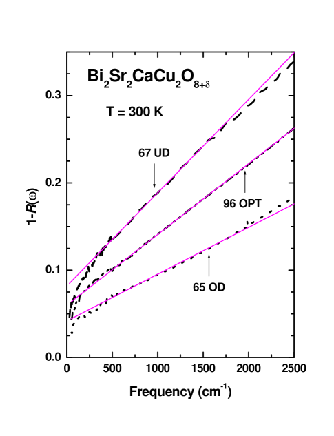
Figure 1: Absorption ($1-R$) data at 300 K for Bi₂Sr₂CaCu₂O_8+δ at three representative doping levels: one underdoped ($T_{c}=67$ K) sample, one optimally-doped ($T_{c}=91$ K) sample, and one overdoped ($T_{c}=65$ K) sample and their linear fits, shown as solid lines. We note that both the slope and the intercept of $1-R$ decrease as the doping level increases.

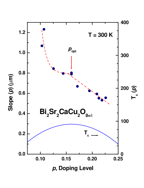
Figure 2: Doping dependent slope of the absorption curves shown in Fig. 1, $S(p)$, of Bi₂Sr₂CaCu₂O_8+δ a 300 K. We observe two different trends: a rapid drop of slope with doping in the underdoped region and a slower linear variation in the overdoped region with a crossover point at $p=p_{opt}=0.16$. The $T_{c}$ vs. $p$ curve shows where our systems are in the phase diagram.

We determined the doping level $p$ from $T_{c}$ using the parabolic expression of Presland et al.presland91 The expression is $p(T_{c})=0.16\mp[{1}/{82.6}\,(1-{T_{c}}/{T_{c}^{max}})]^{1/2}$, where $T_{c}^{max}$ is the maximum $T_{c}$ or $T_{c}(p=0.16)$ and $\mp$ means that we use $-$ for underdoped samples and $+$ for overdoped samples. The determination of $T_{c}^{max}$ is a delicate problemeisaki02 and, in the absence of a better method, we use the generally accepted value of 91 K as the $T_{c}^{max}$ for Bi-2212. We should mention here that we have one optimally-doped sample which is doped with additional small amount of Y to yield a relatively well ordered system and shows a surprisingly high $T_{c}=96$ K eisaki02 . The disadvantage of the Presland method is that it does not uniquely determine the doping level of the sample since there are two independent $p$ values for each value of $T_{c}$. However, as Fig. 1 shows, the reflectance slopes vary monotonically with doping and provide an alternate method of determining the doping level that does not suffer from this ambiguity.

As a first step, we fit the $1-R$ data to a straight line in the frequency range between 500 and 1750 cm^-1 to get the slopes and intercepts at various doping levels. Fig. 2 shows the doping dependence of the slope, $S(p)$ obtained from the $1-R$ curves this way. We note the smooth variation of the slope as the doping level changes. Two different trends can be discerned: a rapid decrease in the underdoped region and a slower decreasing trend in the overdoped region.

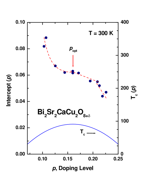
Figure 3: Doping dependent intercept, $I(p)$, of Bi₂Sr₂CaCu₂O_8+δ at 300 K from the fits (see Table 2). We observe three different trends: an abrupt decay in the underdoped region, a slow drop between $p=p_{opt}=0.16$ and $p=p_{c}=0.21$, and an abrupt drop above $p=p_{c}$ as the doping level increases. We observe two crossover points at $p=p_{opt}$ and $p=p_{c}$. We also show the $T_{c}$ vs. $p$ curve.

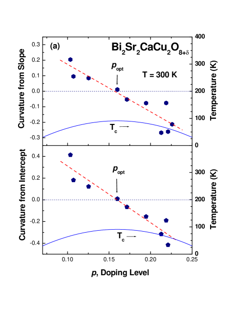
Figure 4: Two doping dependent curvature of $1-R$ of Bi₂Sr₂CaCu₂O_8+δ at 300 K. The curvatures of the $1-R$ curves go through zero at optimal doping where $p=0.16$ (see Sec. II-B for a detailed description).

Fig. 3 shows a doping dependent intercept, $I(p)$ of $1-R$ on the $\omega=0$ axis. The intercept is related to the scattering rate at $\omega=0$ and to the dc resistivity. The intercept also changes smoothly as the doping level changes. The intercepts are consistent with the slopes within the MFL hypothesis, except at the high doping range, where we observe a hint of a crossover around $p=0.21$. There are three regions: a sharp decaying trend in the underdoped region similar to what we observed in the slope, a slower decrease in the optimally doped region similar to what we observed in the variation of the slope. At $p\geq 0.21$ we see a crossover where is the intercept drops more abruptly, i.e., the scattering rate drops quickly.

We found another interesting doping dependent trend: a slight deviation from a straight line reflectance in the relaxation region giving rise to a curvature of the reflectance data. We analyze the curvatures of $1-R$ at various doping levels in the following way: We take two frequency segments, $500-1250$ cm^-1 and $1500-2250$ cm^-1 in the relaxation region. Then we fit each segment to a straight line. Next we get slopes and intercepts of the two fitted straight lines. We label these $S_{L}$ and $I_{L}$ (of the lower frequency section) and $S_{H}$ and $I_{H}$ (of the higher frequency section). We estimate two curvatures independently for each $1-R$ curve: $C_{S}=({S_{L}-S_{H}})/{S_{L}}$ from the slopes and $C_{I}=-({I_{L}-I_{H}})/{I_{L}}$ from the intercepts. Fig. 4 shows the two doping dependent curvatures. A positive (negative) curvature stands for an upward convex (concave) curve. As the figure shows, the curvature of $1-R$ is positive for the underdoped samples, negative for the overdoped samples and goes through zero exactly at optimal doping where $1-R$ is a straight line.

II.3 Analysis of $1-R$

The trends which we observe in Fig. 1, the linear variation of the scattering rate with frequency and the overall decrease in the slopes and intercepts with doping, can be related to the parameters of the MFL theory where the scattering rate, $1/{\tau}({\omega},p)\approx$ ${\lambda}(p)[{\omega}+{\pi}T]$, where $\lambda$ is the coupling constant, $p$ is a doping level, and $T$ is the temperature.MFL2

For thick enough superconducting samples the absorbance ($A$) is $1-R$. In the relaxation regime we have the following:

$$A({\omega},p)=\frac{2}{\omega_{p}(p)\tau(\omega,p)}=\frac{2\lambda_{S}(p)}{{\omega}_{p}(p)}{\omega}+\frac{2\ \lambda_{I}(p)\pi T}{{\omega}_{p}(p)}.$$ (1)

The above equation is linear in frequency for a fixed doping level. We get the doping dependent slope, $S(p)$, and intercept, $I(p)$, from a least square fit of our $1-R$ data to a straight line. According to Eq. (1) the slopes and intercepts are related to each other: $\pi TS(p)=I(p)$ and therefore we would obtain the same value of the doping dependent coupling constant $\lambda(p)$ from either the slopes or the intercepts. To account for deviations from Eq. (1) in our approximate analysis we allow the two constants to be different. We call the coupling constants from the slope $\lambda_{S}(p)$ and from the intercept $\lambda_{I}(p)$. Within the MFL hypothesis $\lambda_{S}(p)=\lambda_{I}(p)$. In terms of the measured quantities $S(p)$ and $I(p)$ they are given by:

$$\lambda_{S}(p)=\frac{1}{2}{\omega}_{p}(p)\,S(p),\>\>\>\>\>\>\lambda_{I}(p)=\frac{I(p){\omega_{p}}(p)}{2\pi T}.$$ (2)

To get the absolute value of coupling constants $\omega_{p}(p)$ must be known. We estimate $\omega_{p}(p)$ from the spectral weight of the conductivity below the interband-transition region. To determine the frequency of the onset of interband transitions, we note that the absorption coefficients, $\alpha(\omega)=4\pi\sigma(\omega)/[n(\omega)c]$, begin to deviate from the low frequency form at 9000 cm^-1 and extrapolate to zero at the same frequency (13000 cm^-1) for all the samples, independent of doping, as shown in the upper panel of Fig. 5. This fact suggests the following method of estimating the spectral weight up to the interband transition:

$$\omega_{p}^{2}=\frac{120}{\pi}\left[\int^{9000}_{0}\sigma_{1}(\omega)d\omega+\frac{1}{2}\int^{13000}_{9000}\sigma_{1}(\omega)d\omega\right].$$ (3)

In the lower panel of Fig. 5 we show the resulting plasma frequencies of Bi-2212 at 300 K obtained this way. We see that the plasma frequency increases monotonically as the doping level increases.kenziora_comment

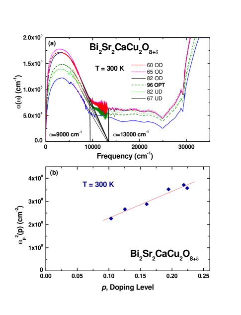
Figure 5: (a) Absorption coefficient $\alpha$ at 300 K for Bi₂Sr₂CaCu₂O_8+δ at six representative doping levels: two underdoped ($T_{c}=67$ and 82 K), one optimally doped ($T_{c}=96$ K), and two overdoped ($T_{c}=82$, 65, and 60 K) samples. (b) Squares of the doping-dependent plasma frequencies $\omega_{p}^{2}$ of Bi-2212 at 300 K, calculated by using Eq. (3). The plasma frequency increases monotonically with doping.

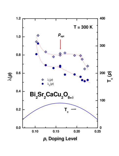
Figure 6: Doping-dependent coupling constants, $\lambda_{S}(p)$ and $\lambda_{I}(p)$, of Bi₂Sr₂CaCu₂O_8+δ at 300 K.

Fig. 6 shows the doping-dependent coupling constants, $\lambda_{S}(p)$ and $\lambda_{I}(p)$ obtained using Eq. (2). Since the doping-dependent plasma frequency increases smoothly with the doping level we see the same trends in $\lambda_{S}(p)$ and $\lambda_{I}(p)$ that we observed in the doping-dependent slope and intercept. We note that the coupling constant $\lambda_{I}(p)$ is larger than $\lambda_{S}(p)$. This is not surprising since in our simple analysis we have neglected the frequency dependence of the plasma frequency required by causality. We correct this in the more complete analysis in the next section. The simple analysis shows an overall trend of a decrease of the dimensionless coupling constants as the doping level increases, which is consistent with the angle-resolved photoemission results.johnson01

II.4 Kubo formula in MFL and Kubo-MFL fit

II.4.1 Reflectance and Kubo-MFL fit

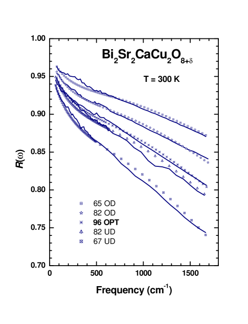
Figure 7: Kubo-MFL fits at 300 K for Bi₂Sr₂CaCu₂O_8+δ at five representative doping levels: two underdoped ($T_{c}=67$ and 82 K), one optimally doped ($T_{c}=96$ K), and two overdoped ($T_{c}=82$ and 65 K) samples. Symbols are fits and solid lines are corresponding data. The fit parameters are shown in Table 1.

Table 1: Kubo-MFL fit parameters of five representative Bi₂Sr₂CaCu₂O_8+δ samples: two underdoped ($T_{c}=67$ and 82 K), one optimally doped ($T_{c}$=96 K), and two overdoped ($T_{c}=82$ and 65 K) samples. The results are shown in Fig. 7.

$T_{c}$ (K)	$\omega_{c}$ (cm-1)	$\lambda_{K}$	$\omega_{p}$ (cm-1)	$\epsilon_{\infty}$
67	2100	0.899	15040	3.14
82	2100	0.720	16320	3.21
96	2100	0.693	16980	3.52
82	2100	0.606	18789	4.16
65	2100	0.457	19270	4.25

Here we introduce a more accurate method of analysis. One can derive the complex optical conductivity from the Kubo formula and the MFL hypothesis as follows.MFL2 ; abrahams96

$$\tilde{\sigma}(\omega)\! = \!-i\frac{\omega_{p}^{2}}{4\pi}\frac{1}{2\omega}\!\int^{\infty}_{-\infty}\!\!\!\!dy[\tanh\frac{\beta\ (y+\omega)}{2}\!-\!\tanh\frac{\beta\ y}{2}]$$ (4)

$$\times[\frac{1}{\Sigma^{R}(y+\omega)-\Sigma^{A}(y)-\omega}],$$

where

$$\Sigma^{R}(\omega) = \lambda\omega\ln\frac{x}{\omega_{c}}-i\frac{\pi\lambda}{2}x,$$

$$\Sigma^{A}(\omega) = \Sigma^{R}(\omega)^{*},$$ (5)

$$x = \max(|\omega|,\pi T).$$

Here $\Sigma^{R}(\omega)$ and $\Sigma^{A}(\omega)$ are the retarded and advanced single-particle self-energies, respectively, $\omega_{c}$ is the cutoff frequency and $\beta\equiv 1/k_{B}T$.

$$\tilde{\epsilon}(\omega) = i\frac{4\pi}{\omega}\tilde{\sigma}(\omega)+\epsilon_{\infty}$$

$$R(\omega) = |\frac{\sqrt{\tilde{\epsilon}(\omega)}-1}{\sqrt{\tilde{\epsilon}(\omega)}+1}|^{2}.$$ (6)

where $\tilde{\epsilon}(\omega)$ is the complex dielectric function, $R(\omega)$ is the reflectance and $\epsilon_{\infty}$ is the background dielectric constant. We will refer to a fit using Eqs. (4),  (II.4.1) and (6) as a “Kubo-MFL fit”. We fixed the plasma frequencies, $\epsilon_{\infty}$ and the cut-off frequency, leaving only $\lambda$ as a free parameter for each doping level.

Fig. 7 shows five representative data sets [$T_{c}=67$ K (UD), $T_{c}=82$ K (UD), $T_{c}=96$ K (OPT), $T_{c}=82$ K (OD), and $T_{c}=65$ K (OD)] and their Kubo-MFL fits between 60 and 1700 cm^-1 and Table 1 shows parameters for the fits. One interesting feature of the fits is that the fitted curves have slight curvature while the reflectance data are straighter. The curvature of the fits above 500 cm^-1 is convex upward (see Sec. II-B) supporting the argument above. The pseudogap induces a concave upward curvature on the reflectance.

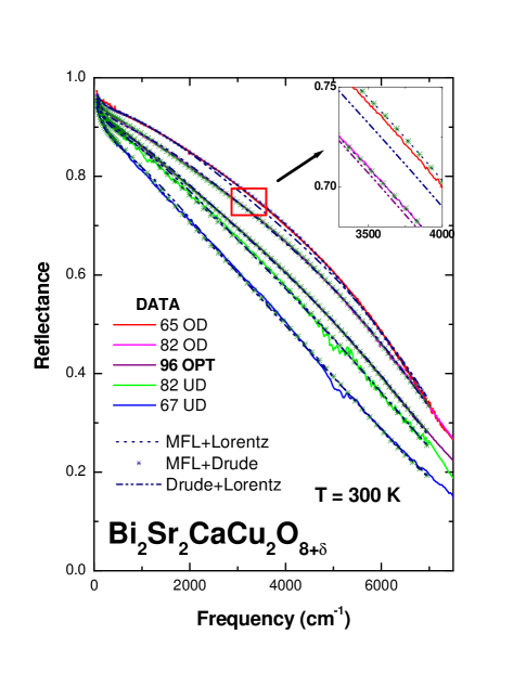
Figure 8: Kubo-MFL fits for extended frequency range at 300 K for Bi₂Sr₂CaCu₂O_8+δ at five representative doping levels: two underdoped ($T_{c}=70$ and 82 K), one optimally doped ($T_{c}=96$ K), and two overdoped ($T_{c}=82$ and 65 K) samples. The symbols (MFL+Drude), dotted lines (MFL+Lorentz) and dash-doulbledotted lines (Drude+Lorentz) are the fits and the solid lines are the corresponding data. The fit parameters are shown in Table 3. The inset shows a magnified view of the fits and demonstrates the need for an MFL contribution for a good fit to the data.

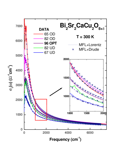
Figure 9: Kubo-MFL fits for extended frequency range at 300 K for Bi₂Sr₂CaCu₂O_8+δ optical conductivity at five representative doping levels: two underdoped ($T_{c}=70$ and 82 K), one optimally doped ($T_{c}=96$ K), and two overdoped ($T_{c}=82$ and 65 K) samples. The symbols (MFL+Drude) and the dotted lines (MFL+Lorentz) are fits and the solid lines are the corresponding data. The fit parameters are shown in Table 3.

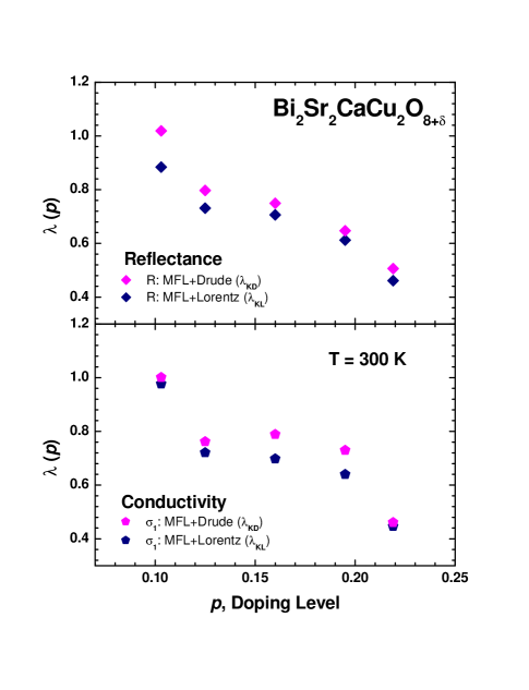
Figure 10: Comparison between two fits: MFL channel + a Drude channel and MFL channel + a Lorentz channel for reflectance and optical conductivity data.

Table 2 shows the slope and intercept for each Bi-2212 sample as well as the coupling constant from the $1-R$ slope analysis between 500 and 1750 cm^-1 for each doping level, as well as the coupling constants from Kubo-MFL fits between 60 and 1700 cm^-1, shown in the $\lambda_{K}(p)$ column.

Table 2: The table shows the sources of 300 K Bi₂Sr₂CaCu₂O_8+δ reflectance $(R)$ data. We fit the $1-R$ data to a straight line in the frequency range between 500 and 1750 cm^-1. The slope and intercept of the fits are shown in the table. The sample whose $T_{c}$ is 96 K is in its optimal doping state. It was assigned a doping level of 0.16. We also show the coupling constants from Kubo-MFL fits between 60 and 1700 cm^-1 in the table.

$T_{c}(K)$	$p$	slope ($\mu$m)	intercept	$\lambda_{S}(p)$	$\lambda_{K}(p)$	Ref.
67	0.103	1.069	0.0818	0.809	0.899	biu70,
70	0.107	1.232	0.0884	0.927	1.165	puchkov96b,
82	0.125	0.844	0.0670	0.688	0.720	puchkov96b,
89	0.144	0.796	0.0620	0.657	0.658
91	0.160	0.790	0.0630	0.670	0.702	tu02,
96	0.160	0.803	0.0616	0.681	0.693	new,eisaki02,
90	0.172	0.669	0.0616	0.585	0.606	puchkov96b,
82	0.195	0.625	0.0555	0.587	0.606	new,eisaki02,
73	0.209	0.594	0.0550	0.561	0.584	new
70	0.213	0.552	0.0520	0.524	0.533	puchkov96b,
65	0.219	0.537	0.0418	0.517	0.457	new
60	0.226	0.564	0.0470	0.526	0.506	new

We were unable to get a fit to the data up to 7000 cm^-1 with the simple MFL parameterization of the data. To get a reasonable fit for an extended range of frequencies we have to add a parallel Drude channel to the conductivity. We fit the same Bi-2212 data at 300 K from 60 to 7000 cm^-1 by adding one Drude oscillator. Here we have three free parameters: the coupling constant $\lambda$, width and strength of the Drude oscillator $\gamma_{D}$ and $\omega_{pD}$. Fig. 8 shows the data and Kubo-MFL fits for the extended spectral range and Table 3 shows parameters for the fits. We observe that the coupling constants [$\lambda_{KD}(p)$] are slightly higher than those [$\lambda_{K}(p)$] of the previous Kubo-MFL fits without oscillators. The spectral weight of the Drude oscillator needed for the good fit shown in the figure ranges from 44 % of the MFL spectral weight for the underdoped sample down to 17 % for the highly overdoped sample. The monotonic variation of the added Drude component with doping suggests that the deviations from the MFL form at high frequency may have a physical significance.

We also fit the same data between 60 and 7000 cm^-1 with the MFL channel and one Lorentz oscillator. Here we have four free parameters: the coupling constant $\lambda$, center frequency, width and strength of the Lorentz oscillator $\omega_{L}$, $\gamma_{L}$ and $\omega_{pL}$. Fig. 8 shows the data and Kubo-MFL fits for the extended spectral range and Table 4 shows parameters for the fits. The spectral weight of the Lorentz oscillator needed for the good fit shown in the figure ranges from 38 % of the MFL spectral weight for the underdoped sample down to 13 % for the highly overdoped sample. We also calculate the mean square deviation $\chi^{2}$ of the two high frequency fits to compare the qualities of the fits. The results are shown in Table 6. With one additional fit parameter the MFL+Lorentz yields a slight improvement in the fit. The exact physical meaning of the additional Drude or Lorentz oscillator is not clear but deviations from the simple MFL parametrization is expected once the energies begin to approach the widths of the bands. In Fig. 10 we show the resulting coupling constants, $\lambda_{KD}(p)$ with $\lambda_{KL}(p)$ for both reflectance and the optical conductivity (see the following subsection).

We fit the same reflectance data between 60 and 7000 cm^-1 with a Drude channel and one Lorentz channel. The fit parameters and resulting fits are shown in Table 5 and Fig. 8, respectively. Interestingly in the two overdoped samples ($T_{c}=82$ K and $T_{c}=65$ K) the least square fits converge to two Drude oscillators even though we start with one Drude and one Lorentz oscillator. We also show the mean square deviations $\chi^{2}_{DL}$ in Table 6. Even though the Drude+Lorentz has the largest number of parameters it shows the worst fit. This suggests that an MFL channel is necessary for a good fit to the Bi-2212 data and probably other cuprates as well.

Table 3: The MFL+Drude fit parameters of five representative Bi₂Sr₂CaCu₂O_8+δ samples: two underdoped ($T_{c}=67$ and 82 K), one optimally doped ($T_{c}$=96 K), and two overdoped ($T_{c}=82$ and 65 K) samples for both reflectance and conductivity. The results of the fits are shown in Fig. 8 and  9. We have added to the MFL conductivity channel (plasma frequency $\omega_{p}$) a Drude channel with a plasma frequency $\omega_{pD}$ and a width $\gamma_{D}$. In the table ”($R$)” and ”($\sigma_{1}$)” stand for the reflectance and the conductivity, respectively.

$T_{c}$ (K)	$\omega_{c}$ (cm-1)	$\lambda_{KD}$	$\omega_{p}$ (cm-1)	$\epsilon_{\infty}$	$\gamma_{D}$	$\omega_{pD}$
67 ($R$)	7100	1.019	15040	3.14	4790	9970
82 ($R$)	7100	0.797	16320	3.21	4250	9360
96 ($R$)	7100	0.749	16980	3.52	4000	9960
82 ($R$)	7100	0.647	18789	4.16	3300	10260
65 ($R$)	7100	0.506	19270	4.25	2930	7920
67 ($\sigma_{1}$)	7100	1.001	15040	3.14	3980	10843
82 ($\sigma_{1}$)	7100	0.762	16320	3.21	3270	10397
96 ($\sigma_{1}$)	7100	0.789	16980	3.52	2708	10987
82 ($\sigma_{1}$)	7100	0.730	18789	4.16	2013	11400
65 ($\sigma_{1}$)	7100	0.461	19270	4.25	2569	9497

Table 4: The MFL+Lorentz fit parameters of five representative Bi₂Sr₂CaCu₂O_8+δ samples: two underdoped ($T_{c}=67$ and 82 K), one optimally doped ($T_{c}$=96 K), and two overdoped ($T_{c}=82$ and 65 K) samples for both reflectance and conductivity. The results of the fits are shown in Fig. 8 and  9. We have added to the MFL conductivity channel (plasma frequency $\omega_{p}$) a Lorentz channel with a center frequency $\omega_{L}$, a plasma frequency $\omega_{pL}$ and a width $\gamma_{L}$. In the table ”($R$)” and ”($\sigma_{1}$)” stand for the reflectance and the conductivity, respectively.

$T_{c}$ (K)	$\omega_{c}$ (cm-1)	$\lambda_{KL}$	$\omega_{p}$ (cm-1)	$\epsilon_{\infty}$	$\omega_{L}$	$\gamma_{L}$	$\omega_{pL}$
67 ($R$)	7100	0.884	15040	3.14	1229	5161	9344
82 ($R$)	7100	0.731	16320	3.21	1003	4600	8910
96 ($R$)	7100	0.706	16980	3.52	801	4177	9614
82 ($R$)	7100	0.612	18789	4.16	741	3470	9851
65 ($R$)	7100	0.461	19270	4.25	1472	3436	6944
67 ($\sigma_{1}$)	7100	0.977	15040	3.14	373	4115	10765
82 ($\sigma_{1}$)	7100	0.721	16320	3.21	503	3585	10216
96 ($\sigma_{1}$)	7100	0.698	16980	3.52	606	3007	10533
82 ($\sigma_{1}$)	7100	0.640	18789	4.16	492	2322	10853
65 ($\sigma_{1}$)	7100	0.447	19270	4.25	463	2722	9555

Table 5: The Drude+Lorentz fit parameters of five representative Bi₂Sr₂CaCu₂O_8+δ samples: two underdoped ($T_{c}=67$ and 82 K), one optimally doped ($T_{c}$=96 K), and two overdoped ($T_{c}=82$ and 65 K) samples for reflectance. The results of the fits are shown in Fig. 8. We have five fit parameters: two from a Drude channel with a plasma frequency $\omega_{pD}$ and a width $\gamma_{D}$ and three from a Lorentz channel with a center frequency $\omega_{L}$, a plasma frequency $\omega_{pL}$ and a width $\gamma_{L}$.

$T_{c}$ (K)	$\epsilon_{\infty}$	$\gamma_{D}$	$\omega_{pD}$ (cm-1)	$\omega_{L}$	$\gamma_{L}$	$\omega_{pL}$
67 ($R$)	3.14	698	9149	2336	8762	13200
82 ($R$)	3.21	618	10300	2201	8493	13323
96 ($R$)	3.52	607	10810	2022	7343	13187
82 ($R$)	4.16	625	11958	0.14	6950	14735
65 ($R$)	4.25	444	12268	0.12	6040	14491

Table 6: Comparison between three fits for reflectance data: MFL channel + a Drude channel, MFL channel + a Lorentz channel and a Drude channel + a Lorentz channel. We named the mean square deviations $\chi^{2}_{MD}$ for the MFL+Drude fit, $\chi^{2}_{ML}$ for the MFL+Lorentz fit, and $\chi^{2}_{DL}$ for the Drude+Lorentz. The additional parameters of the Lorentz fit yields only a slight improvement when we compare the MFL+Lorentz fit with the MFL+Drude fit.

$T_{c}$ (K)	$\chi^{2}_{MD}$	$\chi^{2}_{ML}$	$\chi^{2}_{DL}$
67	18.65	17.03	21.45
82	16.35	15.63	18.62
96	2.21	1.48	6.59
82	3.61	2.89	6.14
65	7.99	6.57	43.70
No. of parameters	3	4	5

II.4.2 Conductivity and Kubo-MFL fit

We also fit the optical conductivity between 60 and 7000 cm^-1 with an MFL channel and two different oscillators: MFL + Drude or MFL + Lorentz. We determined the optical conductivity from the measured reflectance by using a Kramers-Kronig analysis wooten72 , for which extrapolations to $\omega\rightarrow 0\>\>\mbox{and}\>\>\infty$ must be supplied. For $\omega\rightarrow 0$, the reflectance was extrapolated by assuming a Hagen-Rubens frequency dependence, $(1-R)\propto\omega^{1/2}$. The reflectance has been extended to high-frequency by using a literature data tarasaki90 and free-electron behavior ($R\propto\omega^{-4}$). The result of the fits to the data are shown in Fig. 8 and the fit parameters are given in Table 3 and  4. We also show the resulting doping dependent coupling constants from two different fits for both reflectance and conductivity in Fig. 9. We observe smoother doping dependent coupling constant in the result from the reflectance fit. This is one of the reasons why we use reflectance to study the doping dependent properties.

The additional Drude and Lorenz oscillators introduced to fit the wider frequency range data should not be taken literally as additional physical channels of conductivity. They only serve to correct the frequency dependence of the MFL spectrum that is known not to fit well over a wider range of frequencies elazrak94 ; baraduc96 ; vanderMarel03 .

III Discussions

We note that as a first approximation, the MFL spectrum of fluctuations accounts for the data well in the low frequency region of $\omega<2000$ cm^-1 both within the simple $1-R$ slope analysis and the more accurate Kubo formalism. In Fig. 11 we compare the dimensionless coupling constants $\lambda(p)$ from the two different methods of analysis: 1-$R$ and Kubo-MFL fit (without oscillators). The coupling constant decreases uniformly with doping except for the highly underdoped samples. However, in the low doping range the pseudogap temperature $T^{*}$ may approach our measurement temperature of 300 K. The pseudogap leads to a decreased scattering rate at low frequencies which would in turn lead to an enhanced slope of the absorption curve. The upturn in the slope at low doping levels may therefore well be a pseudogap effect. Thus, our first conclusion is that at room temperature the coupling constant $\lambda(p)$ decreases uniformly in the doping region that we have studied without any evidence of any crossovers.

We also show in Fig. 11 the coupling constants from the $1-R$ slope analysis and from ARPES.johnson01 Johnson et al.johnson01 argued that in the normal state the self-energy is well described by the MFL hypothesis and in the overdoped region the difference between the superconducting and normal state dispersion vanishes. They calculated the coupling constants by using $\lambda=-(\partial\mbox{Re}\Sigma/\partial\omega)_{E_{F}}$. We have augmented their analysis by estimating the coupling constant at room temperature which is lower than their published low-temperature value in the underdoped region. This is probably due to a rearrangement of spectral weight of the spin-fluctuation spectrum with temperature. As the temperature is lowered, this rearrangement takes two forms: spectral weight is removed from low frequencies as a result of the development of the spin gap but added to intermediate frequencies with the development of the neutron resonance that couples strongly to the carriers. The net result is a strong increase in $\lambda$ which suggests that spectral weight is removed from high frequencies to fill the neutron mode.schachinger03

The overall good agreement of the coupling constant and its doping dependence between the infrared and the ARPES data is surprising since the infrared response represents an average over the Fermi surface, whereas the ARPES data shown in Fig. 11 represents corrections to the self energy in the $(\pi,\pi)$ direction. Also, ARPES measures the particle life-times directly, whereas infrared is weighted in favor of large angle scattering.

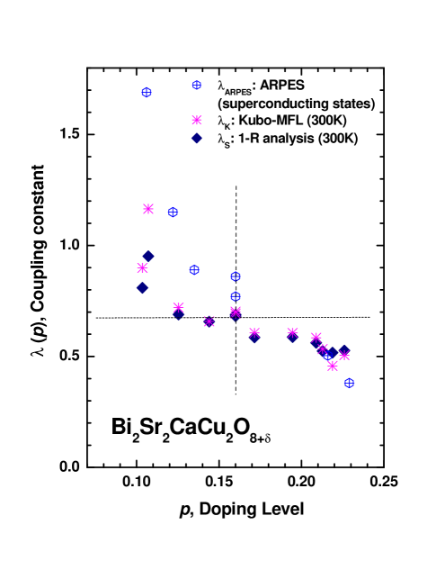
Figure 11: Coupling constants, $\lambda(p)$, of Bi₂Sr₂CaCu₂O_8+δ at 300 K from two different methods, discussed in the text and one result from angle resolved photoemission spectroscopy of Bi-2212 data in the superconducting state.johnson01

Our data on the intercept and the curvature does show evidence of doping-dependent discontinuities. The effect of the pseudogap on the intercept would be opposite from that on the slope, causing it to be smaller at low doping if there was a pseudogap. Instead, as shown in Fig. 3, we observe the opposite effect in the underdoped region, the intercept is higher than what would be expected from a uniformly increasing $\lambda$ with underdoping. Also, in the highly overdoped region the intercept drops, whereas the slope appears to have a more uniform trend in the 0.16 to 0.22 doping region. The overall result of these effects is to produce an S-shaped curve centered at optimal doping.

However, the clearest evidence of a singular doping level at $p=0.16$ comes from our analysis of the doping dependence of the curvature plotted in Fig. 4. Here we see a good fit to a straight line that goes through zero exactly at optimal doping $p=0.16$. This phenomenon is directly related to the well known observation that the dc resistivity in high temperature superconductors varies linearly with temperature only at optimal doping and curved on either side of optimal doping. This was shown by Takagi et al.takagi92 for overdoped and underdoped La_2-xSr_xCuO₄, by Carrington et al. in underdoped YBa₂Cu₃O_7-δ (Ref. carrington93, ), by Kubo et al. in overdoped Tl₂Ba₂CuO₂ (Ref. kubo91, ) and by Konstantinovic et al. for underdoped Bi-2212konstantinovic99 and for underdoped and overdoped Bi₂Sr_1.6La_0.4CuO_ykonstantinovic01 . The present work extends this work to Bi-2212 and covers both overdoped and underdoped materials for the same system. Needless to say, we study the frequency dependence whereas the dc resistivity work is based on the temperature dependence. Thus we show by an independent method that at room temperature the MFL fluctuations are centered at optimal doping $p=0.16$.

IV Conclusions

We have analyzed the 300 K reflectance data of Bi-2212 single crystals at various doping levels from underdoped ($p=0.103$) to highly overdoped ($p=0.226$). We found three smoothly varying quantities with doping, the doping dependent slope, intercept and the curvature of the reflectance in the relaxation region of frequencies. From the smooth trend of the reflectance slope with doping we derive a useful measure of the doping level. We estimate a reliable doping dependent dimensionless coupling constant $\lambda_{S}(p)$ from the $1-R$ slope analysis which varies smoothly from 0.93 to 0.52 in the doping range from $p=0.103$ to 0.226. We also obtained doping dependent curvature of $1-R$. Plotting the curvature as a function of doping we found that the curvature goes through zero at optimal doping.

- (1) P. W. Anderson, in Frontiers and Borderlines in Many-Particle Physics, edited by J. R. Schrieffer and R. A. Broglia (North-Holland, Amsterdam, 1988).
- (2) P. W. Anderson, in Strong Correlation and Superconductivity, edited by H. Fukuyama, S. Mackawa, and A. Malozemoff (Springer-Verlag, Berlin, 1989).
- (3) C. M. Varma, P. B. Littlewood, S. Schmitt-Rink, E. Abrahams, and A.E. Ruckenstein, Phys. Rev. Lett. 63, 1996 (1989).
- (4) M. Gurvitch and A. T. Fiory, Phys. Rev. Lett. 59, 1337 (1987).
- (5) Z. Schlesinger, R. T. Collins, F. Holtzberg, C. Feild, S. H. Blanton, U. Welp, G. W. Crabtree, Y. Fang, and J. Z. Liu, Phys. Rev. Lett. 65, 801 (1990).
- (6) L. D. Rotter, Z. Schlesinger, R. T. Collins, F. Holtzberg, C. Field, U. W. Welp, G. W. Crabtree, J. Z. Liu, Y. Fang, K.G. Vandervoort, and S. Fleshler, Phys. Rev. Lett. 67, 2741 (1991).
- (7) For a review see: T. Timusk and B. Statt, Rep. Prog. Phys. 62, 61 (1999); an update to this review can be found in Ref. 17.
- (8) V. M. Krasnov, cond-mat/0201287 (2002).
- (9) C. Renner, B. Revaz, J. Y. Genoud, K. Kadowaki, and Ø. Fischer, Phys. Rev. Lett. 80, 149 (1998).
- (10) V. M. Krasnov, A. Yurgens, D. Winkler, P. Delsing, and T. Claeson, Phys. Rew. Lett. 84, 5860 (2000).
- (11) M. Suzuki and T. Watanabe, Phys. Rev. Lett. 85, 4787 (2000).
- (12) C. C. Homes, T. Timusk, R. Liang, D. A. Bonn, and W. N. Hardy, Phys. Rev. Lett. 71, 1645 (1993).
- (13) M. Takigawa, A. P. Reyes, P. C. Hammel, J. D. Thompson, R. H. Heffner, Z. Fisk, and K. C. Ott, Phys. Rev. B 43, 247 (1991).
- (14) A. Damascelli, Z. Hussain, and Z.-X. Shen, Rev. Mod. Phys. 75, 473 (2003).
- (15) T. Shibauchi, L. Krusin-Elbaum, Ming Li, M.P. Maley, and P.H. Kes, Phys. Rev. Lett. 86, 5763 (2001).
- (16) A. V. Puchkov, D. N. Basov, and T. Timusk, J. Phys.: Condens. Matter 8, 10049 (1996).
- (17) T. Timusk, cond-mat/0303383 (2002).
- (18) L. Forro, G. L. Carr, G. P. Williams, D. Mandrus, and L. Mihaly, Phys. Rev. Lett. 65, 1941 (1990).
- (19) A. El Azrak, R.Nahoum, N. Bontemps, M. Guilloux-Viry, C. Thivet, A. Perrin, S. Labdi, Z. Z. Li, and H. Raffy, Phys. Rev B 49, 9846 (1994).
- (20) C. Baraduc, A. El Azrak, and N. Bontemps, J. of Superconductivity 9, 3 (1996).
- (21) M. A. Quijada, D. B. Tanner, R. J. Kelley, and M. Onellion, H. Berger, and G. Margaritondo, Phys. Rev. B 60, 14917 (1999).
- (22) J. J. Tu, C. C. Homes, G. D. Gu, D. N. Basov, and M. Strongin, Phys. Rev. B 66, 144514 (2002).
- (23) P. B. Littlewood and C. M. Varma, J. Appl. Phys. 69, 4979 (1991).
- (24) E. Abrahams, J. Phys. I France 6, 2191 (1996).
- (25) A. V. Puchkov, P. Fournier, D. N. Basov, T. Timusk, A. Kapitulnik, N. N. Kolesnikov, Phys. Rev. Lett. 77, 3212 (1996).
- (26) L. Mihaly, C. Kendziora, J. Hartge, D. Mandrus, L. Forró, Rev. of Sci. Inst. 64, 2397 (1993).
- (27) C. C. Homes, M. A. Reedyk, D. A. Crandles, and T. Timusk, Appl. Opt. 32, 2976 (1993).
- (28) T. Timusk and D.B. Tanner, in Physical Properties of High Temperature Superconductors I, edited by D. M. Ginsberg (World Scientific, Singapore, 1989), 341.
- (29) M. R. Presland et al., Phyica C 165, 391 (1991).
- (30) H. Eisaki, N. Kaneko, D. L. Feng, A. Damascell, P. K. Mang, K. M. Shen, M. Greven, and Z. X. Shen, to be published (2002).
- (31) We cannot rule out the possibility here that the spectral weight saturates above optimal doping as suggested by a number of authors. For a summary see A. V. Puchkov, P. Fournier, T. Timusk, and N. N. Kolesnikov, Phys. Rev. Lett. 77, 1853 (1996). See also a comment by C. Kendziora, M. C. Martin, L. Forro, D. Mandrus, and L. Mihaly, Phys. Rev. Lett. 79, 4935 (1997).
- (32) P. D. Johnson, T. Valla, A. V. Fedorov, Z. Yusof, B. O. Wells, Q. Li, A. R. Moodenbaugh, G. D. Gu, N. Koshizuka, C. Kendziora, Sha Jian, and D. G. Hinks, Phys. Rev. Lett. 87, 177007 (2001).
- (33) N. L. Wang, A. W. McConnell, B. P. Clayman, and G. D. Gu, Phys. Rew. B 59, 576 (1999).
- (34) A. V. Puchkov, P. Fournier, T. Timusk, and N. N. Kolesnikov, Phys. Rev. Lett. 77, 1853 (1996).
- (35) Frederick Wooten, Optical Porperties of Solids, Academic, New York (1972).
- (36) I. Terasaki, S. Tajima, H. Eisaki, H. Takagi, K. Uchinokura and S. Uchida, Phys. Rev. B 41, 865 (1990).
- (37) D. van der Marel, H.J.A. Molegraaf, J. Zaanen, Z. Nussinov, F. Carbone, A. Damascelli, H. Eisaki, M. Greven, P.H. Kes, and M. Li, Nature 425, 271 (2003).
- (38) E. Schachinger, J.J. Tu, and J.P. Carbotte, Phys. Rev. B 67, 214508/1-17, (2003).
- (39) H. Takagi et al., Phys. Rev. Lett. 69, 2975 (1992).
- (40) A. Carrington, D. J. C. Walker, A. P. Mackenzie, and J. R. Cooper, Phys. Rev. B 48, 13051 (1993).
- (41) Y. Kubo, Y. Shimakawa, T. Manako, and H. Igarashi, Phys. Rev. B 43, 7875, (1991).
- (42) Z. Konstantinovic, Z.Z. Li, and H. Raffy, Physica B 259-261, 567, (1999).
- (43) Z. Konstantinovic, Z.Z. Li, and H. Raffy, Physica C 351, 163, (2001).