Stable two-dimensional dispersion-managed soliton

Abstract

The existence of a dispersion-managed soliton in two-dimensional nonlinear Schrödinger equation with periodically varying dispersion has been explored. The averaged equations for the soliton width and chirp are obtained which successfully describe the long time evolution of the soliton. The slow dynamics of the soliton around the fixed points for the width and chirp are investigated and the corresponding frequencies are calculated. Analytical predictions are confirmed by direct PDE and ODE simulations. Application to a Bose-Einstein condensate in optical lattice is discussed. The existence of a dispersion-managed matter-wave soliton in such system is shown.

PACS numbers: 05.45.-a, 05.45.Yv, 03.75.Lm

I Introduction

Nonlinear wave propagation in media with periodically varying dispersion is attracting a huge interest over the recent years. A prominent example is a dispersion-managed (DM) optical soliton, which is considered to become the major concept in future soliton-based communication systems. It was shown theoretically and experimentally that the strong DM regime provides the undisturbed propagation of pulses over very long distances. DM solitons are robust to the Gordon-Haus timing jitter, which makes them favorable against the standard solitons [4, 5].

Mathematically this type of problems are described by the one dimensional (1D) nonlinear Schrödinger (NLS) equation with periodic dispersion - a nonlinear analogue of the Mathieu equation. The corresponding linear equation exhibits a rich variety of stability and instability zones for the parameters. The existence of a DM soliton is one of the nontrivial consequences of the stable diagram for the periodic NLS equation.

Although well studied in the 1D case, the two and three dimensional extensions of this problem are far less explored. The major difference here is that, contrary to the 1D case, the NLS equation in two and three dimensions is unstable against collapse. In particular, for the two dimensional (2D) case the collapse occurs if the initial power exceeds some critical value, i.e. if $E>E_{cr}$. Recently it has been demonstrated that the nonlinearity management can prevent the collapse of solitons in 2D Kerr type optical media [6, 7], as well as in 2D Bose-Einstein condensates [8, 9]. From these one can reasonably expect that the dispersion-management can play balancing role also in the 2D case, and the stable 2D DM soliton can exist. Such a possibility has recently been considered in Ref.[10] by construction of the ground state for the periodic 2D NLS equation based on the averaged variational principle and the techniques of integral inequalities - i.e. the proof of the existence theorem for DM soliton was presented. Analytical and numerical treatment of the problem, however, has not been addressed so far.

The purpose of this Communication is to derive analytical expressions for the parameters of a 2D dispersion-managed soliton and to study the conditions for their stability. To this regard, we use a time-dependent variational approach (VA) to derive a set of ODEs for the soliton parameters. The stability of the DM soliton is then inferred from the stability of fixed points of the VA equations.

The field dynamics is governed by the following 2D NLS equation

$$iu_{t}+d(t)\Delta u+|u|^{2}u=0,$$ (1)

where $d(t)=d_{0}+d_{1}(t)$ represents a time periodically varying dispersion coefficient. In the strong DM regime it is assumed that $d(t)\sim(1/\epsilon)d(t/\epsilon),\epsilon\ll 1$ and the dispersion averaged over the period is $<d(t)>=d_{0}$ (in this case $d_{0}>0$ corresponds to a negative dispersion and $d_{0}<0$ to a positive one).

The equation (1) can be associated with two main physical problems: (i) beam propagation in 2D waveguide arrays with periodically variable coupling between waveguides [11, 12]; (ii) nonlinear matter-waves of Bose-Einstein condensates in 2D optical lattices.

In case (i) the model equations for a 2D nonlinear fiber array are given by [13]

$$i\psi_{n,z}+\kappa(z)\Delta_{2}\psi_{n}+\omega^{\prime\prime}\psi_{n,tt}+\chi|\psi_{n}|^{2}\psi_{n}=0,$$ (2)

where $\psi_{n}$ is the envelope of electric field in the n-th fiber, $\Delta_{2}$ is the finite second difference for 2D, $\kappa(z)$ is the variable along $z$ coupling coefficient [11, 12], $\omega^{\prime\prime}$ is the group-velocity dispersion, $\chi$ is the coefficient of nonlinearity. For long wavelength pulses the group-velocity dispersion $\omega^{\prime\prime}$ can be neglected. Introducing the dimensionless variables $\kappa z=t,\psi_{n}=\sqrt{2\kappa/\chi}u_{n}$ and considering the field distribution to be broad in the transverse direction ($>7$ sites), one arrives to Eq. (1) with time and space interchanged and with $d(t)$ describing a varying diffraction along the longitudinal direction. Notice that although the intrinsic discreteness of the array may arrest the collapse of a 2D NLS wave, it does not necessarily stabilize the pulse against decay. In the following we show that this can be done employing dispersion (diffraction) management by means of which a stable 2D soliton can be created before the strong shrinking of the wave occurs.

A similar situation arises in case (ii) for a Bose-Einstein condensates (BEC) confined in a 2D optical lattice. In this case dynamics of the condensate is governed by the Gross-Pitaevskii (GP) equation

$$i\hbar\Psi_{t}=-\frac{\hbar^{2}}{2m}\Delta\Psi+V(x,y;t)\Psi+g_{2D}|\Psi|^{2}\Psi,$$ (3)

where $g_{2D}=g_{3D}/\sqrt{2}\pi a_{z}),g_{3D}=4\pi\hbar^{2}a_{s}/m,a_{z}=(\hbar/m\omega_{z})^{1/2}$ and with $V(x,y)=V_{0}(t)(\cos^{2}(k_{0}x)+\cos^{2}(k_{0}y))$ denoting an optical lattice with the amplitude periodically varying in time. Spatiotemporal wave collapse in the framework of a similar equation (when the potential is periodic in one direction $V(x,y)=V_{0}\cos(k_{0}x)$) was considered in [14], where analytical expression for the upward shift of collapse criterion was derived for potentials rapidly oscillating in space (large $k_{0}$). By adopting an effective mass description one can show that the 2D GP equation [15] can be reduced to the DM NLS equation (1). The effectiveness of DM applied to quasi-1D atomic matter-waves was experimentally demonstrated in Ref.[16].

For analytical considerations it is convenient to refer to the axially symmetric case for which $\Delta=\partial^{2}/\partial r^{2}+(1/r)(\partial/\partial r)$, and apply the harmonic modulation for dispersion-management: $d(t)=d_{0}+d_{1}\sin(\Omega t)$. We remark that although in the present Communication we do not consider the case of two-step dispersion-management: $d(t)=d_{+},\mbox{ if }\ t_{+}+nt_{p}>t>nt_{p},\mbox{ and }d(t)=d_{-},\mbox{ if }(n+1)t_{p}>t>nt_{p}+t_{+}$, where $t_{p}=t_{+}+t_{-},\ \ n=0,1,2...$ , this approach can also be effectively used for the creation of stable 2D DM solitons.

Our analysis of the pulse dynamics under dispersion-management is based on the variational approach [5, 17], according to which a space averaged Lagrangian $\bar{L}=\int Ld{\bar{r}}$ is constructed starting from a suitable ansatz for the soliton profile. In the following we shall calculate $\bar{L}$ by using the following Gaussian ansatz

$$u(r,t)=A(t)\exp(-\frac{r^{2}}{2a^{2}}+i\frac{b(t)r^{2}}{2}+i\phi(t)),$$ (4)

where $A,a,b,\phi$ denote the amplitude, width, chirp and linear phase of the soliton, respectively. The equations for the soliton parameters are then derived from the Euler-Lagrange equations for $\bar{L}$ as

$$a_{t}=2d(t)\beta,\quad\beta_{t}=\frac{2d(t)-E}{a^{3}},$$ (5)

where $\beta=ab$, and $E=\int_{0}^{\infty}|u|^{2}rdr$ is the energy.

II System of averaged variational equations

Let us consider the evolution of a pulse (a beam or a soliton matter-wave, depending on the physical system in consideration) using the division on the fast and slow time scales [18, 19, 20]. The width and chirp of the pulse are then represented as $a(t)=\bar{a}+a_{1},\ \beta(t)=\bar{\beta}+\beta_{1}$, where $\bar{a},\bar{\beta}$ are slowly varying functions on the scale $1/\epsilon$ and $a_{1},\beta_{1}$ are rapidly varying functions. The solutions for $a_{1},\beta_{1}$ are

$$a_{1}=-\frac{4d_{0}d_{1}}{\bar{a}^{3}(\omega_{0}^{2}+\Omega^{2})}\sin(\Omega t)-\frac{2\Omega d_{1}\bar{\beta}}{\omega_{0}^{2}+\Omega^{2}}\cos(\Omega t),$$ (6)

$$\beta_{1}=\frac{6\sigma d_{1}\bar{\beta}}{\bar{a}^{4}(\omega_{0}^{2}+\Omega^{2})}\sin(\Omega t)-\frac{2d_{1}\Omega}{\bar{a}^{3}(\omega_{0}^{2}+\Omega^{2})}\cos(\Omega t),$$ (7)

where $\omega_{0}^{2}=-6\sigma/\bar{a}^{4}$, $\sigma=2d_{0}-E$. Note that $\sigma<0$ for over-critical energy for collapse $E>E_{cr}=2$, at $d_{0}=1$ given by the VA. The exact value, corresponding to the so called ”Townes soliton” is $E_{cr}=1.862$ [21]. Considering the limit of high frequencies $\Omega^{2}\gg\omega_{0}^{2}\sim 1$, for the averaged parameters of the system we finally get

$$\bar{a}_{t}=2\bar{\beta}(d_{0}+\frac{3d_{1}^{2}\sigma}{\Omega^{2}\bar{a}^{4}}),$$ (8)

$$\bar{\beta}_{t}=\frac{\sigma}{\bar{a}^{3}}+\frac{12d_{1}^{2}d_{0}}{\Omega^{2}\bar{a}^{7}}+\frac{12\sigma d_{1}^{2}\bar{\beta}^{2}}{\Omega^{2}\bar{a}^{5}}.$$ (9)

This system has the Hamiltonian structure with the Hamiltonian given by

$$H=\frac{\sigma}{2{\bar{a}}^{2}}+\frac{2\Lambda^{2}d_{0}}{{\bar{a}}^{6}}+\bar{\beta^{2}}(d_{0}+\frac{3\Lambda^{2}\sigma}{\bar{a}^{4}}),\quad\Lambda=\frac{d_{1}}{\Omega},$$ (10)

from which the equations of motion follows as $\bar{a}_{t}=\partial H/\partial\bar{\beta},\ \bar{\beta}_{t}=-\partial H/\partial\bar{a}.$ From this Hamiltonian one can also see that the mechanism for collapse suppression originates from the repulsive potential near the small values of width $\sim 1/\bar{a}^{6}$, which counteracts to the attractive force induced by the nonlinearity $\sim 1/\bar{a}^{2}$. The exact balance between these forces gives rise to a stable state. This state is oscillatory with the frequency which will be defined later. The stabilization mechanism of a 2D NLSE soliton is similar to that of the inverted pendulum with oscillating pivot point [22]. We should note that the averaged dynamics is not potential - a velocity dependent term appears in the interaction potential (see 4th term in (10)). Although this term doesn’t contribute to the fixed point, it is important for the description of oscillatory dynamics of 2D DM solitons.

The system (8),(9) has the fixed points

$$\bar{\beta}=0,\ \bar{a}_{c}=(-\frac{12d_{0}\Lambda^{2}}{\sigma})^{1/4}.$$ (11)

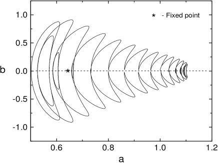
FIG. 1.: Phase portrait of the variational equations (5) with parameters $d_{0}=1,\ d_{1}=3.5,\ \Omega=50,\ E=N/2\pi=2.3034$.

Note that $\Lambda$ is proportional to the strength of the dispersion map $D=2\pi d_{1}/\Omega$, therefore $\bar{a}_{c}\sim\sqrt{D}$ in analogy with the estimate for a DM soliton in 1D case. There exists one solution with a stationary width for the anomalous residual dispersion $d_{0}>0,E>2d_{0}$. This is confirmed by the phase portrait (Fig.1) of the variational system (5).

Let us analyze the stability of fixed points for the anomalous residual dispersion $d_{0}>0$. We assume $a=a_{c}+\epsilon a_{1},\beta=\epsilon\beta_{1}$. Substituting into Eq.(8) and Eq.(9), and collecting terms of order $\epsilon$ we find

$$a_{1,t}=(2d_{0}+\frac{6\Lambda^{2}\sigma}{a^{4}})\beta_{1}=M\beta_{1},$$ (12)

$$\beta_{1,t}=-(\frac{3\sigma}{a^{4}}+\frac{84\Lambda^{2}d_{0}}{a^{8}})a_{1}=-Sa_{1}.$$ (13)

The oscillations of the width and chirp near the fixed points are stable if $MS>0$, which is always satisfied for $d_{0}>0,E>2d_{0}$. The frequency of secondary slow oscillations of a 2D DM soliton is proportional to $\sqrt{MS}$.

III Numerical simulations

To avoid the singularity at $r=0$ we consider the problem in Cartesian coordinates $\Delta=\partial^{2}_{x}+\partial^{2}_{y}$, and $r^{2}=x^{2}+y^{2}$. Then numerical simulations can be performed by two-dimensional fast Fourier transform [23]. The results are produced using a 2D grid of 256 x 256 points over the domain $x,y\in[-6.4,6.4]$ and the time step $\delta t=0.001$. To prevent the back-action of a small amount of linear waves, resulted from the periodic perturbation, the absorption on the domain boundaries is employed, which also imitates the infinite domain condition. The dispersion map was supposed to have parameters $d_{0}=1,\ d_{1}=3.5,\ \Omega=50$.

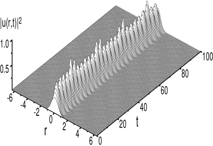
FIG. 2.: Evolution of a 2D DM soliton according to numerical solution of the equation (1). The wave function is normalized to $N=2\pi E_{0}$ with $E_{0}=2.3034$, and the dispersion map is $d_{0}=1,\ d_{1}=3.5,\ \Omega=50.$

This choice of parameters corresponds to moderate dispersion-management ($D\simeq 0.45$). The axial section profile of the wave function $|u(r,t)|^{2}$ as obtained by direct numerical solution of the PDE (1) is presented in Fig.2. As can be seen, rather stable quasi-periodic dynamics is realized for a selected parameter settings. Note that would the periodic modulation of the dispersion had not been applied, the initial waveform would have collapsed within $t\sim 3$. The dispersion-management stabilizes the pulse against the collapse or decay, providing undisturbed propagation over very long distances. The agreement between the predictions of the variational equations (5) for the width of a 2D DM soliton and the corresponding result from the full PDE simulations is reported in Fig.3. As can be observed from this figure, the width of a 2D DM soliton performs quasi-periodic motion with the average width of $\bar{a}\simeq 0.8$ according to variational equations, while the PDE simulation yields $\bar{a}\simeq 0.7$. The fixed point for the above set of parameter values, according to eq.(11) is $\bar{a}_{c}=0.6635$ (see Fig.1). The frequencies of slow dynamics given by the VA equations and PDE are also in well agreement (Fig.3). The estimate for the frequency of slow oscillations from Eq.(12) yields $\omega_{a}=\sqrt{MS}=3.5$, therefore the period is $T_{a}=1.9$. The direct gauge from the Fig.3 shows that $T_{a}\simeq 2.2$, in reasonable agreement with the above VA estimate.

For Bose-Einstein condensates in a 2D optical lattice the dispersion coefficient can be expressed as $d(t)=m/m^{\ast}(t)$ in the effective mass formalism [15]. The effective mass $m^{\ast}$ substantially differs from the true mass $m$ (becoming even negative) and can be varied by changing the parameters of the periodic potential, or inducing the transitions between energy bands.

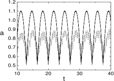
FIG. 3.: Stable quasi-periodic dynamics of the width of a 2D DM soliton. Solid line - variational equations (5) solved for $E=N/2\pi=2.3034$, and the initial conditions $a(0)=1,\ \beta(0)=0$. Dashed line - full PDE simulations of the equation (1).

For example, transitions between the 1st and 2nd bands (at the band edges) in the optical lattice of strength $V_{0}=2.4E_{rec}$ ( where $E_{rec}=\hbar^{2}k_{0}^{2}/2m$ is the recoil energy, $k_{0}=2\pi/\lambda_{0}$, $\lambda_{0}$ is the laser wavelength), leads to variation of the dispersion coefficient in the range $d(t)=(-2.5\div 4.5)$ as considered above.

IV Conclusion

In conclusion, we have demonstrated the possibility to stabilize the 2D soliton with over-critical energy $(E>E_{cr})$ by applying the dispersion-management. The developed theory based on the variational approximation successfully describes the long term evolution of a 2D DM soliton, which is confirmed by direct PDE simulations. We discussed the possible experimental realization of a stable 2D dispersion-managed soliton in Bose-Einsten condensates confined to optical lattices.

REFERENCES

- [1] Electronic address: fatkh@physic.uzsci.net
- [2] Electronic address: baizakov@sa.infn.it
- [3] Electronic address: salerno@sa.infn.it
- [4] N. J. Smith, F. M. Knox, N. J. Doran, K. J. Blow, and I. Bennion, Electronics Letters, 32, 54 (1996).
- [5] I. Gabitov, S. K. Turitsyn, Opt. Lett. 21, 327 (1996).
- [6] L. Berge, V. K. Mezentsev, P. L. Christiansen, Yu. Gaididei, and J. J. Rasmussen, Opt. Lett. 25, 1037 (2000).
- [7] I. Towers, B. A. Malomed, J. Opt. Soc. Am. B 19, 537 (2002).
- [8] F. Kh. Abdullaev, J. G. Caputo, R. Kraenkel, and B. A. Malomed, Phys. Rev. A 67, 013605 (2003).
- [9] H. Saito, M. Ueda, Phys. Rev. Lett. 90, 040403 (2003).
- [10] V. Zharnitsky, E. Grenier, C. K. R. T. Jones, and S. K. Turitsyn, Physica D 152, 794 (2001).
- [11] U. Peschel and F. Lederer, J. Opt. Soc. Am. B 19, 544 (2002).
- [12] S. A. Darmanyan, Opt. Commun. 90, 301 (1992).
- [13] A. B. Aceves, G. Luther, C. De Angekis, A. M. Rubenchik, and S. K. Turitsyn, Phys. Rev. Lett. 75, 73 (1995); Opt. Lett. 19, 329 (1994).
- [14] Y. S. Kivshar and S. K. Turitsyn, Phys. Rev. E 49, R2536 (1994).
- [15] V. V. Konotop and M. Salerno, Phys. Rev. A 65, 021602 (2002); H. Pu, et al. Phys. Rev. A 67, 043605 (2003).
- [16] B. Eiermann, P. Treutlein, Th. Anker, M. Albiez, M. Taglieber, K.-P. Marzlin, M.K. Oberthaler, ArXiv: cond-mat/0304594.
- [17] B. A. Malomed, Progress in Optics, 43, 69 (2002).
- [18] F. Kh. Abdullaev and J. G. Caputo, Phys. Rev. E 58, 6637 (1998).
- [19] S. K. Turitsyn, A. B. Aceves, C. K. R. T. Jones, and V. Zharnitsky, Phys. Rev. E 58, R48 (1998).
- [20] J. Garnier, Opt. Commun. 206, 411 (2002).
- [21] L. Berge, Phys. Rep. 303, 259 (1998).
- [22] L. D. Landau and E. M. Lifshitz, Mechanics, Pergamon Press, Oxford, (1976).
- [23] W. H. Press, S. A. Teukolsky, W. T. Vetterling, and B. P. Flannery, Numerical Recipes. The Art of Scientific Computing. (Cambridge University Press, 1996).