The Correlated Kondo-lattice Model

Abstract

We investigate the ferromagnetic Kondo-lattice model (FKLM) with a correlated conduction band. A moment conserving approach is proposed to determine the electronic self-energy. Mapping the interaction onto an effective Heisenberg model we calculate the ordering of the localized spin system self-consistently. Quasiparticle densities of states (QDOS) and the Curie temperature $T_{\rm C}$ are calculated. The band interaction leads to an upper Hubbard peak and modifies the magnetic stability of the FKLM.

I Introduction

There has been renewed interested in the ferromagnetic Kondo-lattice model ZEN51 (1, 2) since the discovery of the colossal magnetoresistance (CMR) RAM97 (3, 4, 5). This model consists of uncorrelated (s-)band electrons that interact intra-atomically with localized quantum spins (Hund’s rule coupling). Apart from model extensions such as electron-phonon interaction EG01 (5), the role of electronic correlations among the conduction electrons has been emphasized HV00 (6). These correlations are often incorporated as a Hubbard-like interaction, i. e. the conduction electrons interact locally via a repulsive Coulomb matrix element $U$ HUB63 (7). The Hamiltonian of the correlated FKLM reads (for simplicity we assume one ($s$-)orbital):

$$H=\sum_{ij\sigma}T_{ij}c_{i\sigma}^{{\dagger}}c_{j\sigma}-J\sum_{i}\mbox{\boldmath${\sigma}$}_{i}\cdot{\bf S}_{i}+\frac{1}{2}U\sum_{i\sigma}n_{i\sigma}n_{i-\sigma}\;.$$ (1)

As usual, $c_{i\sigma}^{{\dagger}}~{}(c_{i\sigma})$ creates (annihilates) an electron of spin $\sigma~{}(=\uparrow,\downarrow)$ at site $i$, $T_{ij}$ are the hopping integrals, and ${\sigma}$_i and ${\bf S}_{i}$ denote the conduction electron spin and the localized spin, respectively, coupled by an intra-atomic exchange constant $J$. The notion ferromagnetic is due to a positive $J$. The (F)KLM is also known as s-d or s-f model; if the (positive) Hund coupling greatly exceeds the kinetic energy, the double exchange model is obtained ZEN51 (1, 2).

With estimated values of the bandwidth $W\simeq 1-2$ eV, $J\simeq 1$ eV, and $U\simeq 8$ eV for LaMnO₃, as given in SPV96 (8), the Hubbard interaction has certainly to be taken into account. A theory of the (ferromagnetic) correlated Kondo-lattice model should therefore treat both the Hund and the Hubbard interaction as strong couplings. Furthermore, we stress the importance of the quantum character of the localized spins, which is usually neglected FUR98 (4, 6). On the one hand, assuming classical (localized) spins allows for the application of Dynamical Mean Field Theory, a state-of-the-art theory for strongly correlated systems; on the other hand, the influence of electron-magnon interaction (”spin-flips”), which is suppressed when using classical spins, on the electronic spectrum is rather considerable SN02 (9).

We present a theory that accounts for the strong coupling aspect as well as quantum mechanical spins. First, a moment conserving decoupling procedure (MCDA), which has already been applied to the uncorrelated Kondo-lattice model both for bulk and film geometries SN02 (9, 10), yields the electronic self-energy. Secondly, the Hund coupling between localized spins and conduction electrons is mapped onto an effective Heisenberg operator by integrating out the electronic degrees of freedom SN02 (9).

As an extension to the theory for the uncorrelated Kondo-lattice model, our approach incorporates the electron-electron interaction according to the decoupling scheme proposed by Hubbard himself (”Hubbard-I”) HUB63 (7). The modified RKKY interaction is formulated by means of an effective medium method to take care of the additional correlations.

II Theory

For technical details the reader is referred to SN02 (9). The equation of motion (EOM) for the Green’s function $G_{ij\sigma}(E)=\langle\langle c_{i\sigma};c_{j\sigma}^{{\dagger}}\rangle\rangle_{E}$ yields

$$\sum_{l}\left(E\delta_{il}-T_{il}\right)G_{lj\sigma}(E)=\hbar\delta_{ij}+U\Gamma_{iii,j\sigma}(E)-\frac{1}{2}J\left\{z_{\sigma}I_{ii,j\sigma}(E)+F_{ii,j\sigma}(E)\right\},$$ (2)

with $z_{\uparrow}=1,~{}z_{\downarrow}=-1$, and the higher Green’s functions

$${\Gamma}_{ikl,j\sigma}(E)=\langle\langle{c_{i-\sigma}^{{\dagger}}c_{k-\sigma}c_{l\sigma};c^{{\dagger}}_{j\sigma}}\rangle\rangle_{E}\;,$$ (3)

$$I_{ik,j\sigma}(E)=\langle\langle{S_{i}^{z}c_{k\sigma};c^{{\dagger}}_{j\sigma}}\rangle\rangle_{E}~{},~{}~{}~{}~{}~{}F_{ik,j\sigma}(E)=\langle\langle{S_{i}^{-\sigma}c_{k-\sigma};c^{{\dagger}}_{j\sigma}}\rangle\rangle_{E}\;.$$ (4)

One proceeds with writing down again the equations of motion and decouples the resulting still higher Green’s functions. Fortunately, within the frame of the Hubbard-I decoupling, the Hubbard-Green’s function can be expressed as a functional of already known quantities:

$$\Gamma_{iii,j\sigma}(E)={\cal G}\left[G_{ij\sigma}(E),I_{ii,j\sigma}(E),F_{ii,j\sigma}(E)\right]\;.$$ (5)

The higher Green’s functions in the equations of motion of $I_{ik,j\sigma}(E)$ and $F_{ik,j\sigma}(E)$, too, are projected onto $G,\;I,\;{\rm and\;}F$ and in addition, where electron density correlations show up explicitly, onto $\Gamma$. The coefficients are fixed via sum rules. From this closed system of equations, one obtains an electronic self-energy of the following structure:

$$\Sigma_{ij\sigma}(E)={\cal S}\left[\Sigma_{ij\sigma}(E),\langle n_{i\sigma}\rangle,\langle S_{i}^{z}\rangle,\langle(S_{i}^{z})^{2}\rangle,\langle(S_{i}^{z})^{3}\rangle,\langle S_{i}^{\pm}S_{i}^{\mp}\rangle,...\right]\;.$$ (6)

The mapping of the Hund’s rule interaction onto an effective Heisenberg-like spin-spin operator $H_{SS}$ is achieved by averaging it in the subspace of the $s$-electrons. In our case this is done with an effective Hamiltonian MN99 (11) that incorporates the Hubbard interaction as a renormalized kinetic term. The result is an anisotropic Heisenberg Hamiltonian:

$$H_{SS}=-\sum_{i,j}\left\{{\hat{J}}^{(1)}_{ij}\left(S_{i}^{+}S_{j}^{-}+S_{i}^{-}S_{j}^{+}\right)+{\hat{J}}^{(2)}_{ij}S_{i}^{z}S_{j}^{z}\right\}+B_{\rm eff}\sum_{i}S_{i}^{z}\;.$$ (7)

The effective exchange integrals

$${\hat{J}}^{(1)}({\bf q})=-\frac{1}{8}J^{2}{\cal D}_{\bf q}^{\uparrow\downarrow}\;,~{}~{}~{}~{}{\hat{J}}^{(2)}({\bf q})=-\frac{1}{8}J^{2}\sum_{\sigma}{\cal D}_{\bf q}^{\sigma\sigma}$$ (8)

become temperature-dependent via

$${\cal D}_{\bf q}^{\sigma\sigma^{\prime}}=-\frac{1}{\pi N}\Im\int_{-\infty}^{+\infty}{\rm d}Ef_{-}(E)\sum_{\bf k}\left(G_{{\bf k}\sigma^{\prime}}^{(U)}(E)G_{{\bf k}+{\bf q},\sigma}(E)+G_{{\bf k}+{\bf q},\sigma}^{(U)}(E)G_{{\bf k}\sigma^{\prime}}(E)\right).$$ (9)

$\Im$ denotes the imaginary part, $f_{-}(E)$ is the Fermi function, and

$$G_{{\bf k}\sigma}^{(U)}(E)=\frac{\hbar}{E-\epsilon({\bf k})-\Sigma^{(U)}_{{\bf k}\sigma}(E)}\;,B_{\rm eff}=\frac{J}{2\pi N}\Im\int_{-\infty}^{+\infty}{\rm d}Ef_{-}(E)\sum_{\bf k\sigma}z_{\sigma}G_{{\bf k}\sigma}^{(U)}(E),$$ (10)

where $\Sigma^{(U)}_{{\bf k}\sigma}(E)$ is an effective medium ”Hubbard-self-energy part”. For $U=0$ and $J\ll t$, one recovers the conventional RKKY-interaction SN02 (9). The spin expectation values in Eq. (6) are obtained by applying a Tyablikov-decoupling to the EOM of a Green’s function according to Callen (for arbitrary $S$) built with $H_{SS}$ SN02 (9, 12). The same method yields a rather simple formula to calculate the Curie temperature of the system:

$$k_{\rm B}T_{\rm C}\simeq\frac{1}{3}S(S+1)\frac{1}{\frac{1}{N}\sum\limits_{\bf q}\left(\frac{B_{\rm eff}}{\langle S^{z}\rangle}+2({\hat{J}}^{(2)}({\bf 0})-2{\hat{J}}^{(1)}({\bf q}))\right)^{-1}_{T\simeq T_{c}}}\;.$$ (11)

III Results and Discussion

   

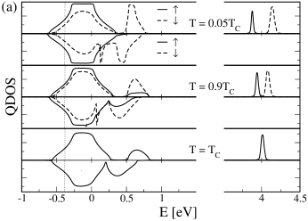
Figure 1: Quasiparticle densities of states. (a) Upper part: $U$ = 4 eV, $T_{\rm C}=144$ K, lower part: $U=0$, $T_{\rm C}=88$ K. Other parameters: $n=0.15$, $J=0.5$ eV, $S=\frac{1}{2}$. (b) Parameters: $J=1$ eV, $S=\frac{3}{2}$. For $n=0$ and $n=1$ the temperature is arbitrary as the system is not self-consistently ferromagnetic.

We investigated the numerical results of our equations on a simple cubic lattice with bandwidth $W=1$ eV, restricting ourselves to ferromagnetism.

In Fig. 1(a) the QDOS is shown at key temperatures in the correlated ($U=4\;$eV) and uncorrelated ($U=0$) case. Note the considerable amount of $\downarrow$-spectral weight even in the ferromagnetically quasi-saturated case (which will not disappear for large $J$, but rather go into saturation on a non-negligible level). The main effect of a finite Hubbard interaction is a removal of spectral weight from the low-energy region, thus creating a gap between the lower subband and the polaron-like second subband. The center of gravity of the latter is shifted to higher energies with increasing $U$. We consider the Stoner-like splitting of the upper Hubbard-band at $E\sim U+\frac{1}{2}JS$ in Fig. 1(a) as an artefact of our approximate theory.

Figure 1(b) shows QDOS for different values of the band occupation in the paramagnetic regime. For finite $U$ and intermediate band occupation, a correlation-induced three-band structure is clearly visible. In the uncorrelated case one observes a shift of the upper band with increasing $n$, changing its character from a polaron-like band (low $n$) to a double-occupation band. Note also the smaller bandwidth in the low energy region for $U=4$ eV due to the reduced effective hopping of the electrons.

Curie temperatures are displayed in Fig. 2. The inset in Fig. 2(a) shows the conventional RKKY-like behaviour $T_{\rm C}\sim J^{2}$ for small $J$ and $n$. A characteristic feature of the modified RKKY theory is, for $n>n_{\rm c}$, a critical value of the Hund coupling $J_{\rm c}$ below which there is no ferromagnetism. It is interesting to note that the critical density $n_{\rm c}$ coincides with the magnetic phase boundary when using conventional RKKY theory. By switching on electronic correlations, we see that the critical interaction $J_{\rm c}$ is shifted to lower values, particularly restoring the system’s ability to exhibit RKKY-ferromagnetism. Furthermore, $T_{\rm C}(J)$ runs into saturation SN02 (9). For $J\gg t$ (in the double exchange regime), there is suppression of ferromagnetic stability due to the Hubbard interaction: as in this regime $T_{\rm C}\sim t$, and a finite $U$ reduces the kinetic energy of the conduction band electrons, $T_{\rm C}$ decreases.

As can be seen in the $T_{\rm C}-n$ phase diagram of Fig. 2(b), the ferromagnetic regime is extended to higher band occupations. However, we did not get any ferromagnetism neither for the uncorrelated nor for the correlated half-filled band. This is consistent with other results WAN98 (13) and with experiment RAM97 (3), where $n\simeq 1$ corresponds to low doping. It goes without saying that our model study does not allow for a detailed comparison with real CMR-materials. Electron-phonon coupling and orbital degeneracy would have to be included, as well as antiferromagnetic calculations to be done. However, the Curie temperature has the right order of magnitude, and runs through a maximum when changing the doping, as observed in RAM97 (3).

In conclusion, we have presented a fully self-consistent theory of the correlated (ferromagnetic) Kondo-lattice model with quantum mechanical spins. The electronic spectrum exhibits a correlation-induced multi-band structure due to the Hubbard interaction, which also modifies the behaviour of the critical temperature. The pronounced suppression of $T_{\rm C}$ for intermediate band occupation (doping) and large Hund coupling indicates that Coulomb correlations should not be neglected when modelling CMR substances.

   

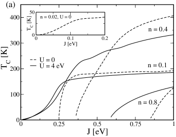
Figure 2: Curie temperatures of the (correlated) Kondo-lattice model ($S=\frac{3}{2}$) as a function of (a) the Hund coupling $J$ and (b) the band occupation $n$.

References

- (1) C. Zener, Phys. Rev. 82, 403 (1951).
- (2) P. W. Anderson and H. Hasegawa, Phys. Rev. 100, 675 (1955).
- (3) A. P. Ramirez, J. Phys. C 9, 8171 (1997).
- (4) N. Furukawa, cond-mat/9812066 (1998).
- (5) D. M. Edwards and A. C. M. Green, cond-mat/0109266v2 (2001).
- (6) K. Held and D. Vollhardt, Phys. Rev. Lett. 84, 5168 (2000).
- (7) J. Hubbard, Proc. R. Soc. London A 276, 238 (1963).
- (8) S. Satpathy, Z. S. Popovic, and F. R. Vukajlovic, Phys. Rev. Lett. 76, 960 (1996).
- (9) C. Santos and W. Nolting, Phys. Rev. B 65, 144419 (2002). See also C. Santos and W. Nolting, Phys. Rev. B 66, 019901(E) (2002).
- (10) R. Schiller and W. Nolting, Phys. Rev. Lett. 86, 3847 (2001).
- (11) D. Meyer and W. Nolting, J. Phys.: Condens. Matter 11, 5811 (1999).
- (12) H. B. Callen, Phys. Rev. 130 890 (1963).
- (13) X. Wang, Phys. Rev. 57 7427 (1998).