Revised Calculation of $\bm{\kappa}_{2}(T)$ for $s$-wave Type-II Superconductors

Abstract

This paper presents revised calculations for the Maki parameters $\kappa_{1}$ and $\kappa_{2}$ and the pair potential $\Delta({\bf r})$ of $s$-wave type-II superconductors near the upper critical field $H_{c2}$ with arbitrary impurity concentration. It is found that Eilenberger’s well-known results on $\kappa_{2}$ [Phys. Rev. 153, 584 (1967)] are not correct quantitatively, which are modified appropriately. Calculations are also performed for a two-dimensional system with an isotropic Fermi surface. The results in the clean limit differ substantially from those in three dimensions with an spherical Fermi surface. This fact indicates the necessity of considering detailed Fermi-surface structures for a quantitative understanding of the parameters. The coefficient of $\Delta({\bf r})\!\propto\!(H_{c2}\!-\!B)^{1/2}$, which is basic to any theoretical evaluation of the thermodynamic and transport properties near $H_{c2}$, is obtained accurately.

I Introduction

Following the preceding studies,Gor'kov59-2 ; Maki64 ; deGennes65 ; Tewordt65 ; HW66 ; WHH66 ; Eilenberger66 ; MT65 ; NT66 ; CCdG66 ; Maki66 EilenbergerEilenberger67 performed an extensive calculation of the parameters $\kappa_{1}(T)$ and $\kappa_{2}(T)$ introduced by MakiMaki64 to distinguish temperature dependences of the upper critical field $H_{c2}$ and the initial slope of the magnetization $\partial M/\partial H$, respectively. Based on the $s$-wave pairing with a spherical Fermi surface and taking both $s$- and $p$-wave impurity scatterings into account, he clarified a basic feature that $\kappa_{2}\!\geq\!\kappa_{1}\!\geq\!\kappa_{\rm GL}$, where $\kappa_{\rm GL}$ is the Ginzburg-Landau parameter near $T_{c}$.GL50 ; FH69 He also found a large dependence of the parameters on the $p$-wave scattering strength. This study is undoubtedly one of the basic works in the field and has been referred to frequently in analyzing experimental results on the quantities. It will be shown, however, that his results on $\kappa_{2}$ are not correct quantitatively due to a couple of inappropriate approximations adopted.

This fact also tells us that we are still far from a quantitative description of type-II superconductors. The parameter $\kappa_{2}$ is such a basic quantity that it is relevant to all thermodynamic and transport properties near $H_{c2}$. Indeed, changes of those quantities through $H_{c2}$ are proportional to the spatial average $\langle|\Delta({\bf r})|^{2}\rangle$ of the pair potential $\Delta({\bf r})$, and $\langle|\Delta({\bf r})|^{2}\rangle$ is directly connected with $\kappa_{2}$, as seen below. Thus, an absence of a reliable theory on $\kappa_{2}$ also implies no quantitative theories for all the other quantities near $H_{c2}$. The exact limiting behaviors would be useful not only for their own sake, but also for getting an insight into the behaviors over $0\!\leq\!B\!\leq\!H_{c2}$. In addition, they would serve as a guide for any detailed numerical studies for $0\!\leq\!B\!\leq\!H_{c2}$.

With these observations, I here perform revised calculations for the Maki parameters and the pair potential near $H_{c2}$. Besides correcting Eilenberger’s results on $\kappa_{2}$ for the spherical Fermi surface, I also perform two-dimensional calculations of the quantities for an isotropic (i.e. cylindrical or circle) Fermi surface. Thereby clarified will be a rather large dependence of $\kappa_{1}(T)$ and $\kappa_{2}(T)$ on detailed Fermi-surface structures. Indeed, even the empirical inequality $\kappa_{2}\!\geq\!\kappa_{1}\!\geq\!\kappa_{\rm GL}$ will be shown violated in some cases in two dimensions, even without the spin paramagnetism.Maki66

The starting point adopted for these purposes is the quasiclassical Eilenberger equations.Eilenberger68 As emphasized by EilenbergerEilenberger68 and also by Serene and Rainer,SR83 the quasiclassical equations have an advantage over Gor’kov equationsGor'kov59 that they are easier to solve due to the absence of an irrelevant energy variable. They have a rigorous microscopic foundation and hence form a firm basis for any quantitative description of superconducting/superfluid Fermi liquids.SR83 Thus, it seems somewhat surprising that few calculations on $\kappa_{2}$ have been performed based on the Eilenberger equations.OB75

This paper is organized as follows. Section II provides the formulation for the $s$-wave pairing with an isotropic Fermi surface and $s$-wave impurity scattering, deferring $p$-wave impurity scattering to Appendix B. The main results are given in Secs. II.5 and II.6, and the differences from Eilenberger’s calculation are explained in Sec. II.8. Section III presents numerical results. Section IV summarizes the paper, with possible extensions to include realistic Fermi surfaces from first-principles calculations and/or anisotropic pairings. Appendix A derives an analytic expression for the magnetization.

II formulation

II.1 Eilenberger equations

I consider the $s$-wave pairing with an isotropic Fermi surface and $s$-wave impurity scattering in an external magnetic field ${\bf H}\parallel\!{\bf z}$. The vector potential in the bulk can be written asEilenberger64 ; Lasher ; Marcus ; Brandt ; DGR90 ; Kita98

$${\bf A}({\bf r})\!=\!Bx\hat{\bf y}\!+\tilde{\bf A}({\bf r})\,,$$ (1)

where $B$ is the average flux density produced jointly by the external current outside the sample and the supercurrent inside it, and $\tilde{\bf A}$ expresses the spatially varying part of the magnetic field satisfying $\int{\bm{\nabla}}\!\times\!\tilde{\bf A}\,d{\bf r}\!=\!{\bf 0}$. I adopt the units where the energy, the length, and the magnetic field are measured by the zero-temperature energy gap $\Delta(0)$ at $H\!=\!0$, the coherence length $\xi_{0}\!\equiv\!\hbar v_{\rm F}/\Delta(0)$ with $v_{\rm F}$ the Fermi velocity, and $B_{0}\!\equiv\!\phi_{0}/2\pi\xi_{0}^{2}$ with $\phi_{0}\!\equiv\!hc/2e$ the flux quantum, respectively. I also put $\hbar\!=\!k_{\rm B}\!=\!1$ and use the gauge where ${\bf\nabla}\cdot\tilde{\bf A}\!=\!0$. The Eilenberger equationsEilenberger68 now read

$$\left[\varepsilon_{n}+\frac{\langle g\rangle}{2\tau}+\frac{\hat{\bf v}}{2}\!\cdot\!\left({\bm{\nabla}}-i{\bf A}\right)\right]f=\left(\Delta+\frac{\langle f\rangle}{2\tau}\right)g\,,$$ (2a)

$$\Delta({\bf r})\ln\!\frac{T_{c}}{T}=-2\pi T\sum_{n=0}^{\infty}\left[\langle f(\varepsilon_{n},{\bf k}_{\rm F},{\bf r})\rangle-\frac{\Delta({\bf r})}{\varepsilon_{n}}\right]\,,$$ (2b)

$$-{\nabla}^{2}\tilde{\bf A}({\bf r})\!=-\frac{i}{\kappa_{0}^{2}}2\pi T\sum_{n=0}^{\infty}\langle\hat{\bf v}\,g(\varepsilon_{n},{\bf k}_{\rm F},{\bf r})\rangle\,.$$ (2c)

Here $\varepsilon_{n}\!\equiv\!(2n+1)\pi T$ is the Matsubara frequency, $\tau$ is the relaxation time in the second-Born approximation, $\langle\cdots\rangle$ denotes the Fermi-surface average satisfying $\langle 1\rangle\!=\!1$, $\Delta({\bf r})$ is the pair potential, and the unit vector $\hat{\bf v}\!=\!\hat{\bf k}$ specifies a point on the isotropic Fermi surface. The quasiclassical Green’s functions $f$ and $g$ are connected by $g\!=\!(1\!-\!ff^{\dagger})^{1/2}$ with $f^{\dagger}(\varepsilon_{n},{\bf k}_{\rm F},{\bf r})\!\equiv\!f^{*}(\varepsilon_{n},-{\bf k}_{\rm F},{\bf r})$, and the dimensionless parameter $\kappa_{0}$ is defined by

$$\kappa_{0}\!\equiv\!{\phi_{0}}/{2\pi\xi_{0}^{2}H_{c}(0)}\,,$$ (3)

where $H_{c}(0)\!\equiv\!\sqrt{4\pi N(0)}\Delta(0)$ is the thermodynamic critical field at $T\!=\!0$ with $N(0)$ the density of states per spin and per unit volume. Equations (2a)-(2c) are to be solved self-consistently for a fixed $B$. Finally, the missing connection between $H$ and $B$ is obtained by applying the Doria-Gubernatis-Rainer scaling DGR89 to Eilenberger’s free-energy functional. Eilenberger68 The details are given in Appendix A. The final result is given by

$$H=B+\frac{1}{BV}\int\!d{\bf r}\,({\bm{\nabla}}\!\times\!\tilde{\bf A})^{2}$$

$$+\frac{\pi T}{2BV\kappa_{0}^{2}}\!\sum_{n=0}^{\infty}\int\!d{\bf r}\left<\!\frac{f^{\dagger}\hat{\bf v}\!\cdot\!({\bm{\nabla}}\!-\!i{\bf A})f\!-\!f\hat{\bf v}\!\cdot\!({\bm{\nabla}}\!+\!i{\bf A})f^{\dagger}}{1+g}\!\right>,$$

(4)

where $V$ is the volume of the system.

II.2 Expansion near $H_{c2}$

Near $H_{c2}$, the coupled equations (2) and (4) are expanded in terms of $\Delta({\bf r})$ as follows. First, let us rewriteKita98

$$\frac{\hat{\bf v}}{2}\!\cdot\!\left({\bm{\nabla}}-i{\bf A}\right)=\frac{\sqrt{B}\sin\theta}{2\sqrt{2}}\left[{\rm e}^{-i\varphi}(a\!+\!\tilde{A})-{\rm e}^{i\varphi}(a^{\dagger}\!+\!\tilde{A}^{*})\right],$$ (5)

where $(\theta,\varphi)$ are the polar angles of $\hat{\bf v}$, and the quantities $a$, $a^{\dagger}$, and $\tilde{A}$ are defined by

$$\left\{\begin{array}[]{l}\vspace{2mm}\displaystyle a\equiv\frac{1}{\sqrt{2B}}\left(\frac{\partial}{\partial x}+i\frac{\partial}{\partial y}+Bx\right)\\ \displaystyle a^{\dagger}\equiv\frac{1}{\sqrt{2B}}\left(-\frac{\partial}{\partial x}+i\frac{\partial}{\partial y}+Bx\right)\end{array}\right.,$$ (6a)

$$\tilde{A}\!\equiv\!-i\frac{\tilde{A}_{x}+i\tilde{A}_{y}}{\sqrt{2B}}\,,$$ (6b)

with $[a,a^{\dagger}]\!=\!1$. The operators $(a,a^{\dagger})$ are the same as $(a_{-},a_{+})$ introduced by Helfand and Werthamer,HW66 and $(F_{-},F_{+})$ by Eilenberger.Eilenberger67

I then expand $f$, $g$, and $\tilde{A}$ up to the third order in $\Delta({\bf r})$ as

$$\left\{\begin{array}[]{l}\vspace{2mm}f=f^{(1)}+f^{(3)}\\ \vspace{2mm}g=1-\frac{1}{2}f^{(1)\dagger}f^{(1)}\\ \tilde{A}\!=\!\tilde{A}^{(2)}\end{array}\right..$$ (7)

Substituting Eqs. (5) and (7) into Eq. (2a) and collecting terms of the same orders, we obtain

$$\bigl{[}\,\tilde{\varepsilon}_{n}+\beta\,({\rm e}^{-i\varphi}a-{\rm e}^{i\varphi}a^{\dagger})\,\bigr{]}f^{(1)}=\Delta+\frac{\langle f^{(1)}\rangle}{2\tau}\,,$$ (8a)

$$\bigl{[}\,\tilde{\varepsilon}_{n}+\beta\,({\rm e}^{-i\varphi}a-{\rm e}^{i\varphi}a^{\dagger})\,\bigr{]}f^{(3)}=\frac{\langle f^{(3)}\rangle}{2\tau}$$

$$-\frac{f^{(1)\dagger}f^{(1)}}{2}\left(\!\Delta+\frac{\langle f^{(1)}\rangle}{2\tau}\!\right)+\frac{\langle f^{(1)\dagger}f^{(1)}\rangle}{4\tau}f^{(1)}$$

$$-\beta\,({\rm e}^{-i\varphi}\tilde{A}^{(2)}-{\rm e}^{i\varphi}\tilde{A}^{(2)*})f^{(1)}\,,$$ (8b)

with

$$\tilde{\varepsilon}_{n}\equiv\varepsilon_{n}+\frac{1}{2\tau},\hskip 14.22636pt\beta\equiv\frac{\sqrt{B}\sin\theta}{2\sqrt{2}}.$$ (9)

Also, Eq. (2b) is transformed into

$$\Delta({\bf r})\ln\!\frac{T_{c}}{T}=-2\pi T\sum_{n=0}^{\infty}\left[\langle f^{(1)}\rangle+\langle f^{(3)}\rangle-\frac{\Delta({\bf r})}{\varepsilon_{n}}\right]\,.$$ (10)

The Maxwell equation (2c) is given in the leading order by

$$-\nabla^{2}\tilde{A}^{(2)}=\frac{\pi T}{\sqrt{2B}\kappa_{0}^{2}}\sum_{n}\langle f^{(1)\dagger}f^{(1)}{\rm e}^{i\varphi}\sin\theta\rangle\,,$$ (11)

whereas Eq. (4) becomes

$$H-B=\frac{\pi T}{2\sqrt{2B}\kappa_{0}^{2}V}\sum_{n}\int\!d{\bf r}\,\langle f^{(1)\dagger}({\rm e}^{-i\varphi}a$$

$$-{\rm e}^{i\varphi}a^{\dagger})f^{(1)}\sin\theta\rangle\,.$$ (12)

II.3 Two-dimensional calculations

To investigate the dependence of the Maki parameters on the Fermi-surface structure, calculations will also be performed for a two-dimensional system with an isotropic Fermi surface placed in the $xy$ plane perpendicular to ${\bf B}$. The analytic expressions for this case can be obtained from those of the three dimensions by simply putting $\sin\theta\!\rightarrow\!1$ and omitting the integrations over $\theta$.

II.4 Transformation into algebraic equations

Equations (8) and (10)-(12) are solved with the Landau-level expansion (LLX) methodKita98 by expanding $\Delta$, $f^{(\nu)}$ $(\nu\!=\!1,3)$, and $\tilde{A}^{(2)}$ in terms of periodic basis functions of the flux-line lattice as

$$\Delta({\bf r})=\sqrt{V}\sum_{N=0}^{\infty}\Delta_{N}\,\psi_{N{\bf q}}({\bf r})\,,$$ (13a)

$$f^{(\nu)}(\varepsilon_{n},{\bf k}_{\rm F},{\bf r})=\sqrt{V}\sum_{m=-\infty}^{\infty}\sum_{N=0}^{\infty}f_{mN}^{(\nu)}(\varepsilon_{n},\theta)\,{\rm e}^{im\varphi}\,\psi_{N{\bf q}}({\bf r})\,,$$ (13b)

$$\tilde{A}^{(2)}({\bf r})=\sum_{{\bf K}\neq{\bf 0}}\tilde{A}_{\bf K}^{(2)}\,{\rm e}^{i{\bf K}\cdot{\bf r}}\,.$$ (13c)

Here $N$ denotes the Landau level, ${\bf q}$ is an arbitrary chosen magnetic Bloch vector characterizing the broken translational symmetry of the flux-line lattice and specifying the core locations, and ${\bf K}$ is a reciprocal lattice vector of the magnetic Brillouin zone. See Ref. Kita98, for the explicit expressions of the basis functions $\psi_{N{\bf q}}({\bf r})$; they are essentially equivalent to Eilenberger’s $\psi_{N}({\bf r}|{\bf r}_{0})$ Eilenberger67 and reduces for $N\!=\!0$ to Abrikosov’s solution for the Ginzburg-Landau equations near $H_{c2}$.Abrikosov57 It only suffices to know the properties:

$$\langle\psi_{N{\bf q}}|\psi_{N^{\prime}{\bf q}}\rangle=\delta_{NN^{\prime}}\,,$$ (14a)

$$\left\{\begin{array}[]{l}\vspace{2mm}\displaystyle a\,\psi_{N{\bf q}}\,=\sqrt{N}\,\psi_{N-1{\bf q}}\\ \displaystyle a^{\dagger}\psi_{N{\bf q}}=\sqrt{N\!+\!1}\,\psi_{N+1{\bf q}}\end{array}\right..$$ (14b)

On the other hand, the expansion in ${\bf K}$ in Eq. (13c) was introduced by BrandtBrandt for solving the Ginzburg-Landau equations over $0\!\leq\!B\!\leq\!H_{c2}$. This expansion enables us to integrate the Maxwell equation appropriately so that $\int{\bm{\nabla}}\!\times\!\tilde{\bf A}\,d{\bf r}\!=\!{\bf 0}$ is satisfied automatically.

A simplification results in Eq. (13) for the $s$-wave pairing with an isotropic Fermi surface near $H_{c2}$. Indeed, $\Delta({\bf r})$ can be described excellently with only the lowest Landau level asKita98

$$\Delta({\bf r})=\sqrt{V}\Delta_{0}\,\psi_{0{\bf q}}({\bf r})\,.$$ (15)

Equation (15) has a wide range of applicability over $B\!\gtrsim\!0.1H_{c2}$ both near $T_{c}$ and in the dirty limit. However, the region in the clean limit shrinks as $T\!\rightarrow\!0$ to disappear eventually. It should also be noted that higher Landau levels of $N\!=\!{\rm even}$ become relevant for anisotropic pairings and/or anisotropic Fermi surfaces at low temperatures.

Substituting Eqs. (13b), (13c), and (15) into Eq. (8) and using the orthogonality of ${\rm e}^{im\varphi}$ and $\psi_{N{\bf q}}$, we realize that $f_{mN}^{(\nu)}$ can be written as

$$f_{mN}^{(\nu)}\!=\!\delta_{mN}\Delta_{0}^{\nu}\tilde{f}_{N}^{(\nu)}\,.$$ (16)

Equations (8) and (10)-(12) are thereby transformed into algebraic equations for $\tilde{f}^{(1)}$, $\tilde{f}^{(3)}$, $\Delta_{0}$, $\tilde{A}_{\bf K}^{(2)}$, and $H\!-\!B$ as

$$\sum_{N^{\prime}}\tilde{\cal M}_{NN^{\prime}}\tilde{f}_{N^{\prime}}^{(1)}=\delta_{N0}\left(1+\frac{\langle\tilde{f}_{0}^{(1)}\rangle}{2\tau}\right),$$ (17a)

$$\sum_{N^{\prime}}\tilde{\cal M}_{NN^{\prime}}\tilde{f}_{N^{\prime}}^{(3)}=\delta_{N0}\frac{\langle\tilde{f}_{0}^{(3)}\rangle}{2\tau}+J_{N}^{(3)}+J_{N}^{(A)}\,,$$ (17b)

$$\ln\frac{T_{c}}{T}=-2\pi T\sum_{n=0}^{\infty}\left(\langle\tilde{f}_{0}^{(1)}\rangle+\langle\tilde{f}_{0}^{(3)}\rangle\Delta_{0}^{2}-\frac{1}{\varepsilon_{n}}\right),$$ (17c)

$$\tilde{A}^{(2)}_{\bf K}=-\frac{2\pi T\Delta_{0}^{2}}{\kappa_{0}^{2}K^{2}}\sum_{n=0}^{\infty}\sum_{N}\frac{J_{N}^{(2)}(\varepsilon_{n})I_{N+1N}({\bf K})}{\sqrt{N\!+\!1}}\,,$$ (17d)

$$H-B=\frac{2\pi T\Delta_{0}^{2}}{\kappa_{0}^{2}}\sum_{n=0}^{\infty}\sum_{N}J_{N}^{(2)}(\varepsilon_{n})\,.$$ (17e)

Here the matrix $\tilde{\cal M}$ is defined by

$$\tilde{\cal M}_{NN^{\prime}}\equiv\delta_{NN^{\prime}}\tilde{\varepsilon}_{n}+\delta_{N,N^{\prime}-1}\beta\sqrt{N\!+\!1}-\delta_{N,N^{\prime}+1}\beta\sqrt{N}\,,$$ (18)

and $J_{N}$’s are given by

$$J_{N}^{(2)}\equiv\frac{(-1)^{N}}{B}\sqrt{N\!+\!1}\,\langle\tilde{f}^{(1)}_{N+1}\tilde{f}^{(1)}_{N}\beta\rangle\,,$$ (19a)

$$J_{N}^{(3)}\equiv-\frac{1}{2}\!\sum_{N^{\prime}}(-1)^{N^{\prime}}I_{NN^{\prime}N+N^{\prime}0}^{(4)}\,\tilde{f}_{N^{\prime}}^{(1)}\tilde{f}_{N+N^{\prime}}^{(1)}\!\left(\!1\!+\!\frac{\langle\tilde{f}_{0}^{(1)}\rangle}{2\tau}\!\right)$$

$$\hskip 22.76219pt+\frac{1}{4\tau}\sum_{N^{\prime}}(-1)^{N^{\prime}}I_{NN^{\prime}N^{\prime}N}^{(4)}\,\langle\tilde{f}_{N^{\prime}}^{(1)}\tilde{f}_{N^{\prime}}^{(1)}\rangle\tilde{f}_{N}^{(1)}\,,$$ (19b)

$$J_{N}^{(A)}\equiv-\frac{\beta}{\Delta_{0}^{2}}\sum_{{\bf K}\neq{\bf 0}}\bigl{[}I_{N+1N}^{*}({\bf K})\tilde{A}_{\bf k}^{(2)}\tilde{f}_{N+1}^{(1)}$$

$$-I_{NN-1}({\bf K})\tilde{A}_{\bf k}^{(2)*}\tilde{f}_{N-1}^{(1)}\bigr{]}\,,$$ (19c)

withKita98

$$I_{N_{1}N_{2}N_{3}N_{4}}^{(4)}\equiv V\int\psi_{N_{1}{\bf q}}^{*}\psi_{N_{2}{\bf q}}^{*}\psi_{N_{3}{\bf q}}\psi_{N_{4}{\bf q}}d{\bf r}\,,$$ (20a)

$$I_{N_{1}N_{2}}({\bf K})\equiv\int\psi_{N_{1}{\bf q}}^{*}\psi_{N_{2}{\bf q}}{\rm e}^{-i{\bf K}\cdot{\bf r}}d{\bf r}\,.$$ (20b)

Equation (17a) tells us that $\tilde{f}_{N}^{(1)}$ is real; this fact has been used in writing down Eqs. (17b)-(17e). As for $\tilde{f}_{N}^{(3)}$, numerical calculations show that $I^{(4)}$’s appearing in Eq. (19b) are all real for the relevant hexagonal lattice, with

$$\beta_{\rm A}\equiv I^{(4)}_{0000}=1.16\,.$$ (21)

Also, $I_{N+1N}({\bf K})$ can be transformed with partial integrations as

$$I_{N+1N}({\bf K})=\frac{1}{\sqrt{N+1}}\int(a^{\dagger}\psi_{N{\bf q}})^{*}\psi_{N{\bf q}}{\rm e}^{-i{\bf K}\cdot{\bf r}}d{\bf r}$$

$$=\frac{\sqrt{N}}{\sqrt{N+1}}I_{NN-1}({\bf K})+\frac{K_{y}\!-\!iK_{x}}{\sqrt{2B(N+1)}}I_{NN}({\bf K})$$

$$=\frac{K_{y}\!-\!iK_{x}}{\sqrt{2B(N\!+\!1)}}\sum_{N_{1}=0}^{N}I_{N_{1}N_{1}}({\bf K})\,.$$ (22)

Since $I_{NN}({\bf K})$ is real, $J^{(A)}$ is also real from Eq. (17d), and so is $\tilde{f}_{N}^{(3)}$.

It is desirable for a later purpose to express $J^{(A)}$ in terms of $I^{(4)}$ rather than $I_{N+1N}({\bf K})$. This can be performed by first substituting Eq. (17d) into Eq. (19c), and then using Eq. (22) and the identity $\sum_{{\bf K}\neq{\bf 0}}{\rm e}^{i{\bf K}\cdot({\bf r}-{\bf r}^{\prime})}\!=\!V\delta({\bf r}\!-\!{\bf r}^{\prime})\!-\!1$. The result is given by

$$J_{N}^{(A)}=\frac{\pi T\beta}{B\kappa_{0}^{2}}\sum_{n^{\prime}=0}^{\infty}\sum_{N^{\prime}}J_{N^{\prime}}^{(2)}\bigl{[}\sqrt{N\!+\!1}\,\tilde{f}^{(1)}_{N+1}({\cal I}_{NN^{\prime}}-1)$$

$$-\sqrt{N}\tilde{f}^{(1)}_{N-1}({\cal I}_{N-1N^{\prime}}-1)\bigr{]},$$ (23)

where $\tilde{f}^{(1)}_{N\pm 1}\!\equiv\!\tilde{f}^{(1)}_{N\pm 1}(\varepsilon_{n})$, $J_{N^{\prime}}^{(2)}\!\equiv\!J_{N^{\prime}}^{(2)}(\varepsilon_{n^{\prime}})$ is given by Eq. (19a), and ${\cal I}_{NN^{\prime}}$ is an average of $I^{(4)}$ defined by

$${\cal I}_{NN^{\prime}}\equiv\frac{1}{(N+1)(N^{\prime}+1)}\sum_{N_{1}=0}^{N}\sum_{N_{1}^{\prime}=0}^{N^{\prime}}I^{(4)}_{N_{1}N_{1}^{\prime}N_{1}^{\prime}N_{1}}\,.$$ (24)

II.5 Solutions

We are now ready to solve Eqs. (17a) and (17b). To this end, let us define

$$\tilde{K}^{N^{\prime}}_{N}\equiv(\tilde{\cal M}^{-1})_{NN^{\prime}}=(-1)^{N+N^{\prime}}\tilde{K}^{N}_{N^{\prime}}\,,$$ (25)

where the second equality originates from $\tilde{\cal M}_{NN^{\prime}}\!=\!(-1)^{N+N^{\prime}}\tilde{\cal M}_{N^{\prime}N}$. Then Eq. (17a) is transformed into

$$\tilde{f}_{N}^{(1)}={\tilde{K}^{0}_{N}}\left(1+\frac{\langle\tilde{f}_{0}^{(1)}\rangle}{2\tau}\right)\,.$$ (26)

Solving Eq. (26) self-consistently for $\langle\tilde{f}_{0}^{(1)}\rangle$ and substituting the result into Eq. (26), we obtain

$$\tilde{f}_{N}^{(1)}=\frac{{\tilde{K}^{0}_{N}}}{{1-\langle\tilde{K}^{0}_{0}\rangle/2\tau}}\,.$$ (27)

The denominator in Eq. (27) corresponds to the so-called “vertex correction.” Equation (17b) for $\tilde{f}_{N}^{(3)}$ may be handled similarly. Using the symmetry $\tilde{K}^{N}_{0}\!=\!(-1)^{N}\tilde{K}^{0}_{N}$, we thereby arrive at the expression for the relevant quantity $\langle\tilde{f}_{0}^{(3)}\rangle$ in Eq. (17c) as

$$\langle\tilde{f}_{0}^{(3)}\rangle=\sum_{N}(-1)^{N}\langle\tilde{f}_{N}^{(1)}(J_{N}^{(3)}\!+\!J_{N}^{(A)})\,\rangle\,.$$ (28)

The quantity $\sum_{N}(-1)^{N}\langle\tilde{f}_{N}^{(1)}J_{N}^{(A)}\rangle$ in Eq. (28) may be transformed further by using Eq. (23) and (19a) as

$$\sum_{N}(-1)^{N}\langle\tilde{f}_{N}^{(1)}(\varepsilon_{n})J_{N}^{(A)}(\varepsilon_{n})\rangle$$

$$=\frac{1}{\kappa_{0}^{2}}\sum_{N}J_{N}^{(2)}(\varepsilon_{n})\,2\pi T\!\!\sum_{n^{\prime}=0}^{\infty}\sum_{N^{\prime}}J_{N^{\prime}}^{(2)}(\varepsilon_{n^{\prime}})({\cal I}_{NN^{\prime}}\!-\!1)\,.$$ (29)

We next consider the self-consistency equation (17c) for the pair potential. Here, $\tilde{f}_{N}^{(1)}(B)$ is expanded in terms of the distance $H_{c2}\!-\!B$ from $H_{c2}$ as

$$\tilde{f}_{N}^{(1)}(B)=\tilde{f}_{N}^{(1)}(H_{c2})-\tilde{f}_{N}^{(1)\prime}(H_{c2})(H_{c2}\!-\!H\!+\!H\!-\!B)\,,$$ (30)

whereas the higher-order term $\tilde{f}_{N}^{(3)}$ is evaluated at $H_{c2}$. To find an explicit expression for $\tilde{f}_{N}^{(1)\prime}$ in Eq. (30), let us differentiate Eq. (17a) with respect to $B$:

$$\sum_{N^{\prime}}\tilde{\cal M}_{NN^{\prime}}\tilde{f}_{N^{\prime}}^{(1)\prime}=\delta_{N0}\frac{{\langle\tilde{f}_{0}^{(1)\prime}\rangle}}{2\tau}$$

$$\hskip 28.45274pt-\frac{\beta}{2B}(\sqrt{N\!+\!1}\tilde{f}_{N+1}^{(1)}-\sqrt{N}\tilde{f}_{N-1}^{(1)})\,.$$ (31)

This equation can be solved in the same way as Eq. (17a) to yield

$$\langle\tilde{f}_{0}^{(1)\prime}\rangle=-\sum_{N}J_{N}^{(2)}\,,$$ (32)

where $J_{N}^{(2)}$ is defined by Eq. (19a). Let us substitute Eqs. (28)-(30) and (32) into Eq. (17c), replace $H\!-\!B$ by the right-hand side of Eq. (17e), and regard $H_{c2}\!-\!H$ as second order. Collecting first-order terms, we obtain the equation to fix the upper critical field $H_{c2}$ as

$$\ln\frac{T_{c}}{T}=-2\pi T\sum_{n=0}^{\infty}\left[\langle\tilde{f}_{0}^{(1)}(\varepsilon_{n})\rangle-\frac{1}{\varepsilon_{n}}\right].$$ (33)

The third-order terms determine the pair potential $\Delta_{0}$ and the magnetization $H\!-\!B$ as a function of $H_{c2}\!-\!H$ as

$$\Delta_{0}^{2}=\frac{H_{c2}\!-\!H}{\kappa_{0}^{2}S_{4}/S_{2}^{2}-S_{A}/S_{2}^{2}}\,\frac{\kappa_{0}^{2}}{S_{2}}\,,$$ (34a)

$$H-B=\frac{H_{c2}\!-\!H}{\kappa_{0}^{2}S_{4}/S_{2}^{2}-S_{A}/S_{2}^{2}}\equiv\frac{H_{c2}\!-\!H}{(2\kappa_{2}^{2}-1)\beta_{\rm A}}\,,$$ (34b)

where $S_{2}$, $S_{4}$, and $S_{A}$ are defined by

$$S_{2}\equiv 2\pi T\sum_{n=0}^{\infty}\sum_{N=0}^{\infty}J_{N}^{(2)}(\varepsilon_{n})\,,$$ (35a)

$$S_{4}\equiv-2\pi T\sum_{n=0}^{\infty}\sum_{N=0}^{\infty}(-1)^{N}\langle\tilde{f}_{N}^{(1)}(\varepsilon_{n})J_{N}^{(3)}(\varepsilon_{n})\rangle\,,$$ (35b)

$$S_{A}\equiv(2\pi T)^{2}\sum_{n=0}^{\infty}\sum_{n^{\prime}=0}^{\infty}\sum_{N=0}^{\infty}\sum_{N^{\prime}=0}^{\infty}J_{N}^{(2)}(\varepsilon_{n})J_{N^{\prime}}^{(2)}(\varepsilon_{n^{\prime}}){\cal I}_{NN^{\prime}}\,,$$ (35c)

with $\tilde{f}_{N}^{(1)}$, $J_{N}$, and ${\cal I}_{NN^{\prime}}$ given by Eqs. (27), (19), and (24), respectively. All the quantities in Eq. (35) are to be evaluated at $H_{c2}$. The latter equality in Eq. (34b) defines the Maki parameter $\kappa_{2}$ with $\beta_{\rm A}\!\equiv\!I^{(4)}_{0000}\!=\!1.16$.

Equation (34) forms the main result of the paper, which is not only exact but also convenient for numerical calculations. An extension to include $p$-wave impurity scattering is carried out in Appendix B, where it is shown that Eq. (34) is still valid with the replacements of $\tilde{f}^{(1)}_{N}$ and $J^{(3)}_{N}$ by Eqs. (75) and (76), respectively.

Sometimes it is physically more meaningful to express $\Delta_{0}$ as a function of $B$ instead of $H$, because $B$ is the real average field inside the bulk directly relevant to the spatial profile of the pair potential. It is obtained, without the replacement of $H\!-\!B$ mentioned above Eq. (33), as

$$\Delta_{0}^{2}=\frac{H_{c2}\!-\!B}{\kappa_{0}^{2}S_{4}/S_{2}^{2}-S_{A}/S_{2}^{2}+1}\,\frac{\kappa_{0}^{2}}{S_{2}}\,.$$ (36)

II.6 Calculation of $\tilde{K}^{N^{\prime}}_{N}$

The key quantity in Eq. (34) is $\tilde{K}^{N^{\prime}}_{N}$ defined by Eq. (25), as may be seen from Eqs. (27), (19), and (35). An efficient algorithm to calculate them is obtained as follows.

Let us define ${\cal D}_{N}$ ($\bar{{\cal D}}_{N}$) for $N\!=\!0,1,2,\cdots$ as the determinant of the submatrix obtained by removing (retaining) the first $N$ rows and columns of the tridiagonal matrix $\tilde{\cal M}$ of Eq. (18), namely,

$${\cal D}_{N}\equiv\det\!\left[\begin{array}[]{cccc}\tilde{\varepsilon}_{n}&\sqrt{N\!+\!1}\,\beta&0&\cdots\\ -\sqrt{N\!+\!1}\,\beta&\tilde{\varepsilon}_{n}&\sqrt{N\!+\!2}\,\beta&\cdots\\ 0&-\sqrt{N\!+\!2}\,\beta&\tilde{\varepsilon}_{n}&\cdots\\ \cdots&\cdots&\cdots&\cdots\\ \end{array}\right],$$ (37a)

$$\bar{\cal D}_{N}\equiv\det\!\left[\begin{array}[]{ccccc}\tilde{\varepsilon}_{n}&\sqrt{1}\,\beta&\cdots&\cdots&\cdots\\ -\sqrt{1}\,\beta&\tilde{\varepsilon}_{n}&\cdots&\cdots&\cdots\\ \cdots&\cdots&\cdots&\cdots&\cdots\\ \cdots&\cdots&\cdots&\tilde{\varepsilon}_{n}&\sqrt{N\!-\!1}\,\beta\\ \cdots&\cdots&\cdots&-\sqrt{N\!-\!1}\,\beta&\tilde{\varepsilon}_{n}\\ \end{array}\right].$$ (37b)

They satisfy

$${\cal D}_{N-1}=\tilde{\varepsilon}_{n}{\cal D}_{N}+N\beta^{2}{\cal D}_{N+1}\,,$$ (38a)

$${\bar{\cal D}}_{N+1}=\tilde{\varepsilon}_{n}{\bar{\cal D}}_{N}+N\beta^{2}{\bar{\cal{\cal D}}}_{N-1}\,,$$ (38b)

as shown by expanding Eqs. (37a) and (37b) with respect to the first and last row, respectively. Aitken56 Then $\tilde{K}^{N^{\prime}}_{N}$ for $N^{\prime}\!\leq\!N$ is obtained by also using standard techniques to solve linear equations Aitken56 as

$$K^{N^{\prime}}_{N}\!=\!\beta^{N-N^{\prime}}\sqrt{\frac{N!}{N^{\prime}!}}\,\frac{{\cal D}_{N+1}{\bar{\cal D}}_{N^{\prime}}}{{\cal D}_{0}}\,.$$ (39)

This algorithm can put into a more convenient form in terms of

$${\cal R}_{N}\equiv\tilde{\varepsilon}_{n}{\cal D}_{N+1}/{\cal D}_{N}\,,$$ (40a)

$$\bar{\cal R}_{N}\equiv\tilde{\varepsilon}_{n}\bar{\cal D}_{N-1}/\bar{\cal D}_{N}\,.$$ (40b)

They satisfy

$${\cal R}_{N-1}=\frac{1}{1+Nb^{2}{\cal R}_{N}}\,,$$ (41a)

$$\bar{\cal R}_{N+1}=\frac{1}{1+Nb^{2}\bar{\cal R}_{N}}\,,$$ (41b)

with $\bar{\cal R}_{1}\!=\!1$ and

$$b\equiv\beta/\tilde{\varepsilon}_{n}\,.$$ (42)

Then $\tilde{K}^{N}_{N}$ and $\tilde{K}^{N^{\prime}}_{N}$ for $N^{\prime}\!<\!N$ are obtained by

$$\tilde{K}^{0}_{0}={\cal R}_{0}/\tilde{\varepsilon}_{n}\,,$$ (43a)

$$\tilde{K}^{N}_{N}=({\cal R}_{N}/\bar{\cal R}_{N})\tilde{K}^{N-1}_{N-1}\,,$$ (43b)

$$\tilde{K}^{N^{\prime}}_{N}=\sqrt{N}\,b\,{\cal R}_{N}\tilde{K}^{N^{\prime}}_{N-1}\,.$$ (43c)

Numerical calculations of ${\cal R}_{N}$ may be carried out by starting from ${\cal R}_{N_{\rm{cut}}}=1$ for an appropriately chosen large $N_{\rm{cut}}$ and using Eq. (41a) to decrease $N$. One can check the convergence by increasing $N_{\rm cut}$. It turns out that $N_{\rm cut}\!=\!1$ is sufficient both near $T_{c}$ and in the dirty limit, thereby reproducing the analytic results by Gor’kov Gor'kov59 and Caroli, Cyrot, and de Gennes,CCdG66 respectively. In contrast, $N_{\rm cut}\!\gtrsim\!1000$ is required in the clean limit at low temperatures.

Noting that Eq. (33) with Eq. (27) should be equivalent to the equation for $H_{c2}$ obtained by Helfand and Werthamer,HW66 we get an alternative expression for $\tilde{K}^{0}_{0}$ as

$$\tilde{K}^{0}_{0}(\tilde{\varepsilon}_{n},\beta)=\sqrt{\frac{2}{\pi}}\int_{0}^{\infty}\!\frac{\tilde{\varepsilon}_{n}}{\tilde{\varepsilon}_{n}^{2}+x^{2}\beta^{2}}\,{\rm e}^{-x^{2}/2}\,dx\,.$$ (44)

The equivalence between Eqs. (43a) and (44) can also be checked numerically.

II.7 Expression of $\kappa_{\rm GL}$

Near $T_{c}$ where $\beta\!\ll\!\tilde{\varepsilon}_{n}$ holds, we may choose $N_{\rm cut}\!=\!1$ in Eqs. (41)-(43) and expand the resulting expressions with respect to $\beta/\tilde{\varepsilon}_{n}$. This yields $\tilde{K}^{0}_{0}\!\approx\!1/\tilde{\varepsilon}_{n}\!-\!\beta^{2}/\tilde{\varepsilon}_{n}^{3}$ and $\tilde{K}^{0}_{1}\!\approx\!\beta/\tilde{\varepsilon}_{n}^{2}$, so that Eq. (27) can be approximated by $\tilde{f}^{(1)}_{0}\!\approx\!1/\varepsilon_{n}\!-\!(\beta^{2}\varepsilon_{n}\!+\!\langle\beta^{2}\rangle/2\tau)/\varepsilon_{n}^{2}\tilde{\varepsilon}_{n}^{2}$ and $\tilde{f}^{(1)}_{1}\!\approx\!\beta/\varepsilon_{n}\tilde{\varepsilon}_{n}$. Using these results in Eq. (35) and retaining only terms of the leading order in $\beta$, we obtain

$$S_{2}=\frac{1}{2d(\pi T_{c})^{2}}\sum_{n=0}^{\infty}\frac{1}{(2n\!+\!1)^{2}(2n\!+\!1\!+\!1/2\pi\tau T_{c})}\,,$$ (45a)

$$S_{4}=\frac{7\zeta(3)}{8(\pi T_{c})^{2}}\beta_{\rm A}\,,$$ (45b)

$$S_{A}=S_{2}^{2}\beta_{\rm A}\,,$$ (45c)

where $d\!=\!2,3$ is the dimension of the system. Substituting Eq. (45) into Eq. (34b), we find the expression of $\kappa_{\rm GL}\!\equiv\!\kappa_{2}(T_{c})$ as

$$\kappa_{\rm GL}=\frac{d\,\pi T_{c}\sqrt{7\zeta(3)}/2}{\displaystyle\sum_{n}[(2n\!+\!1)^{2}(2n\!+\!1\!+\!1/2\pi\tau T_{c})]^{-1}}\,\kappa_{0}\,.$$ (46)

This expression enables us to eliminate $\kappa_{0}$ in favor of $\kappa_{\rm GL}$.

The case with $p$-wave impurity scattering may be treated similarly by using Eqs. (75) and (76) for $\tilde{f}^{(1)}_{N}$ and $J^{(3)}_{N}$, respectively. The resulting $\kappa_{\rm GL}$ is given by Eq. (46) with a replacement of $\tau$ by the transport lifetime $\tau_{\rm tr}$ defined through

$$\frac{1}{\tau_{\rm tr}}\equiv\frac{1}{\tau}-\frac{1}{\tau_{1}}\,,$$ (47)

in agreement with Eilenberger.Eilenberger67

II.8 Eilenberger’s results

I now clarify the connection with Eilenberger’s well-known results. Eilenberger67 They are obtained by extracting from $I_{N_{1}N_{2}N_{3}N_{4}}^{(4)}$ of Eq. (20a) a part which may be expressed in terms of $\beta_{\rm A}\!=\!1.16$ of Eq. (21).

To see this, let us start from an alternative expression of $I_{N_{1}N_{2}N_{3}N_{4}}^{(4)}$ for $N_{1}\!+\!N_{2}\!=\!N_{3}\!+\!N_{4}$:

$$I_{N_{1}N_{2}N_{3}N_{4}}^{(4)}=\sum_{N_{a}}\frac{V}{2}\sum_{\alpha=1}^{2}|\psi_{N_{a}{\bf 0}\alpha}({\bf 0})|^{2}$$

$$\hskip 8.53581pt\times\langle N_{1}N_{2}|N_{1}\!+\!N_{2}\!-\!N_{a}N_{a}\rangle\langle N_{3}N_{4}|N_{1}\!+\!N_{2}\!-\!N_{a}N_{a}\rangle\,.$$

(48)

Here $\psi_{N_{a}{\bf 0}\alpha}({\bf 0})$ and $\langle N_{1}N_{2}|N_{3}N_{4}\rangle$ are the quasiparticle wave function and the overlap integral defined by Eqs. (3.12) and (3.23) of Ref. Kita98-2, , respectively. This identity can be proved by using Eqs. (3.22) and (3.24) of Ref. Kita98-2, and noting $\psi^{({\rm c})}_{N{\bf q}}({\bf r})\!=\!\psi^{({\rm r})}_{N{\bf q}}(2{\bf r})$ which both denote the present $\psi_{N{\bf q}}({\bf r})$. If we retain only terms of $N_{a}\!=\!0$ in Eq. (48) and use $\frac{V}{2}\sum_{\alpha=1}^{2}|\psi_{0{\bf 0}\alpha}({\bf 0})|^{2}\!=\!\beta_{\rm A}$, we obtain an approximate expression for Eq. (48) as

$$I_{N_{1}N_{2}N_{3}N_{4}}^{(4)} \approx\beta_{\rm A}\langle N_{1}N_{2}|N_{1}\!+\!N_{2}0\rangle\langle N_{3}N_{4}|N_{1}\!+\!N_{2}0\rangle$$ (49)

$$=\frac{(N_{1}\!+\!N_{2})!}{2^{N_{1}+N_{2}}\sqrt{N_{1}!N_{2}!N_{3}!N_{4}!}}\,\beta_{\rm A}$$

$$\equiv I_{N_{1}N_{2}N_{3}N_{4}}^{(4{\rm E})}\,.$$

Now, Eilenberger’s approximation for $\kappa_{2}$ is given by Eqs. (2.7), (2.8), and (6.5) of his paperEilenberger67 and corresponds to

$$\kappa_{2}\approx(\kappa_{0}^{2}S_{4}^{({\rm E})}/2S_{2}^{2}\beta_{\rm A})^{1/2}\equiv\kappa_{2}^{({\rm E})}\,,$$ (50)

in Eq. (34b), where $S_{4}^{({\rm E})}$ is obtained from Eq. (35b) by replacing $I^{(4)}$ by $I^{(4{\rm E})}$. Indeed, this procedure yields numerical agreements with his results. As seen below in Sec. III.2, however, this approximation is not correct quantitatively far beyond his estimation $\sim\!1\%$.

It should also be noted that Eilenberger’s definition of $\kappa_{2}$ by Eq. (50) is different from Maki’s through Eq. (34b) with respect to

$$\eta\equiv S_{A}/S_{2}^{2}\beta_{\rm A}\,.$$ (51)

I resume Maki’s definition through Eq. (34b) where $\kappa_{2}$ has a one-to-one correspondence with the initial slope of the magnetization. This is certainly more preferable than expressing the slope with two parameters, $\kappa_{2}^{(E)}$ and $\eta$.

I finally comment on Eilenberger’s analytic expression for $\eta$. In addition to the approximation (49), it was obtained by integrating the Maxwell equation with a removal of a common operator; see the argument above Eq. (6.4).Eilenberger67 However, this procedure may bring an erroneous constant. Indeed, his $B_{0}({\bf r})$ of Eq. (6.4) does not satisfy the required condition $\int B_{0}({\bf r})\,d{\bf r}\!=\!0$. Thus, his expression for $\eta$ is incorrect in the two respects and cannot be obtained by adopting the approximation (49) in Eq. (51).

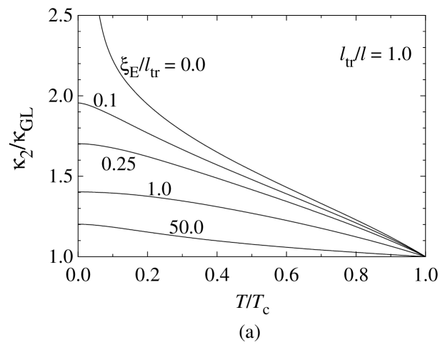
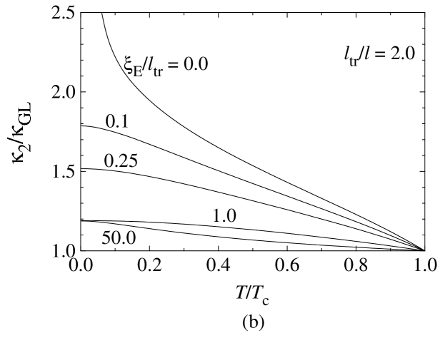
Figure 1: Temperature dependence of $\kappa_{2}/\kappa_{\rm GL}$ for several values of $\xi_{\rm E}/l_{\rm tr}$ in the extreme type-II case $\kappa_{\rm GL}\!=\!50$. (a) $l_{\rm tr}/l=1.0$; (b) $l_{\rm tr}/l=2.0$.

III Numerical Results

III.1 Numerical procedures

I have adopted the same parameters as those of Eilenberger:Eilenberger67

$$\xi_{\rm E}/l_{\rm tr}\equiv 1/2\pi T_{c}\tau_{\rm tr}\,,\hskip 14.22636ptl_{\rm tr}/l\equiv\tau_{\rm tr}/\tau\,,$$ (52)

to express different impurity concentrations. Numerical calculations of Eqs. (33)-(35) have been performed for each set of parameters by restricting every summation over the Matsubara frequencies for those satisfying $\varepsilon_{n}\!\leq\!\varepsilon_{c}$. Choosing $\varepsilon_{c}\!=\!50\!\sim\!100$ has been sufficient to obtain an accuracy of $\sim\!0.01\%$ for $\kappa_{2}$. On the other hand, summations over the Landau levels have been truncated at $N\!=\!N_{\rm cut}$ where I put ${\cal R}_{N_{\rm cut}}\!=\!1$ in the calculation of $K_{N}^{N^{\prime}}$; see Sec. II.6 for the details. Enough convergence has been obtained by choosing $N_{\rm cut}\!=\!4$, $40$, $100$, $200$, $500$, and $2000$ for $\xi_{\rm E}/l_{\rm tr}\!=\!50$, $1.0$, $0.5$, $0.1$, and $0.05$, respectively. Finally, integrations over $\theta$ have been performed by Simpson’s formula with $N_{\rm cut}\!+\!1$ integration points for $0\!\leq\!\theta\!\leq\!\pi/2$.

III.2 Results for $\kappa_{2}$

Figure 1 shows $\kappa_{2}/\kappa_{\rm GL}$ as a function of $T/T_{c}$ for different impurity concentrations. The upper one is for $l_{\rm tr}/l\!=\!1.0$, i.e., the case without $p$-wave impurity scattering, whereas the lower one is for $l_{\rm tr}/l\!=\!2.0$. They are calculated in an extreme type-II case of $\kappa_{\rm GL}\!=\!50$, so that they directly correspond to Eilenberger’s results for $l_{\rm tr}/l\!=\!1$ and $2$, respectively.Eilenberger67 These curves show qualitatively the same behaviors as those of Eilenberger’s, including the divergence in the clean limit for $T\!\rightarrow\!0$, as predicted by Maki and Tsuzuki. MT65 Except the curves in the dirty limit, however, marked quantitative differences are seen. For example, $\kappa_{2}(T\!=\!0)/\kappa_{\rm GL}$ for $(\xi_{\rm E}/l_{\rm tr},l_{\rm tr}/l)\!=\!(1.0,1.0)$ is $1.40$ from the present calculation, whereas it is $1.50$ from Eilenberger’s. Thus, we realize that Eilenberger’s approximation (50) yields quantitative errors of $\lesssim 20\%$ for the deviation $\kappa_{2}/\kappa_{\rm GL}\!-\!1$. Comparing the two figures, we observe the followings: (i) The results in the dirty limit are the same between $l_{\rm tr}/l\!=\!1$ and $2$; (ii) $p$-wave scattering has a general tendency to lower the values of $\kappa_{2}$, and also produces a non-monotonic behavior in $\kappa_{2}/\kappa_{\rm GL}$ as a function of $\xi_{\rm E}/l_{\rm tr}$.

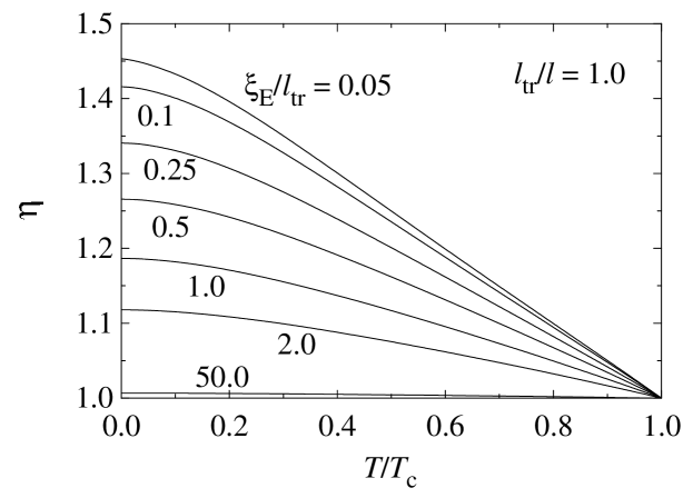
Figure 2: Temperature dependence of $\eta$ defined by Eq. (51) for several values of $\xi_{\rm E}/l_{\rm tr}$ with $l_{\rm tr}/l\!=\!1.0$.

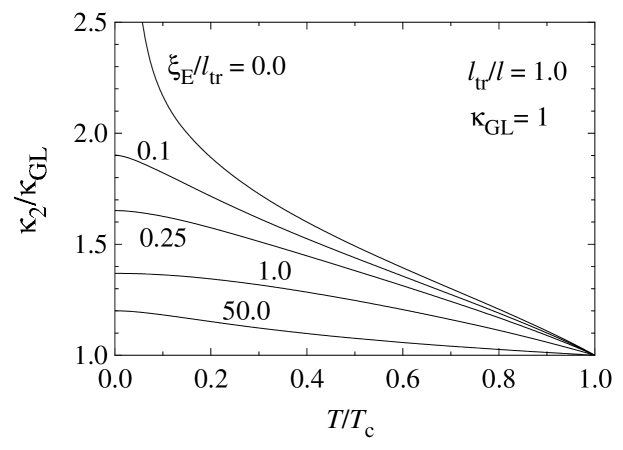
Figure 3: Temperature dependence of $\kappa_{2}/\kappa_{\rm GL}$ for $\kappa_{\rm GL}\!=\!1$ with $l_{\rm tr}/l=1.0$.

Figure 2 displays $\eta$ defined by Eq. (51) as a function of $T/T_{c}$ for $\xi_{\rm E}/l_{\rm tr}\!=\!0.05$-$50.0$ and $l_{\rm tr}/l\!=\!1.0$. This quantity becomes relevant for small values of $\kappa_{\rm GL}$ at low temperatures, as may be realized by Eq. (34b). The curves also deviate substantially from Eilenberger’s results. For example, $\eta$ for $\xi_{\rm E}/l_{\rm tr}\!=\!0.25$ at $T\!=\!0$ is $1.34$ from the present calculation, whereas it is $\sim\!1.11$ from Eilenberger’s. Generally, the values are larger than those of Eilenberger’s. This fact implies that $\kappa_{2}(T)$ for $\kappa_{\rm GL}\!\sim\!1$ becomes smaller than the evaluation of Eilenberger.

To see the dependence of $\kappa_{2}/\kappa_{\rm GL}$ on $\kappa_{\rm GL}$ explicitly, I have performed a calculation of $\kappa_{2}$ near the type-I-type-II boundary of $\kappa_{\rm GL}\!=\!1.0$. Figure 3 plots the results for $\xi_{\rm E}/l_{\rm tr}\!=\!0.0$-$50.0$ and $l_{\rm tr}/l\!=\!1$. Compared with Fig. 1(a), we observe that each curve is slightly shifted downward. However, the changes are surprisingly small, considering the closeness to the type-I-type-II boundary. We thus realize that the factor $S_{A}/S_{2}^{2}\!=\!\eta\beta_{\rm A}$ in Eq. (34b) can be neglected practically for $\kappa_{\rm GL}\!\gtrsim\!5$, as already observed by Eilenberger.Eilenberger67

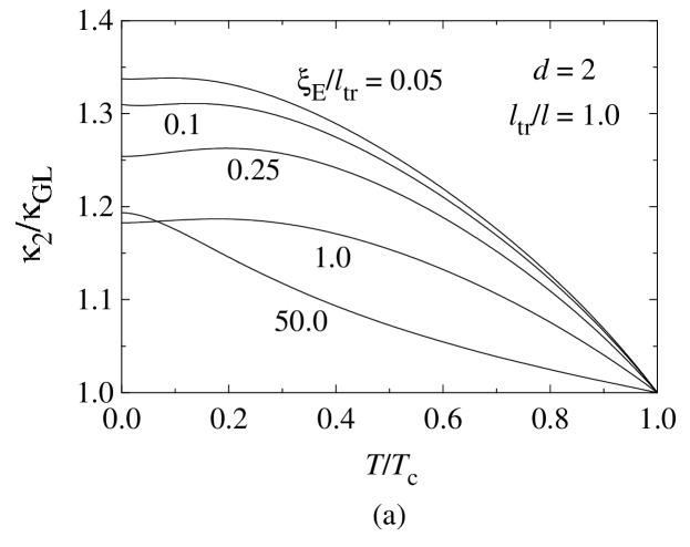
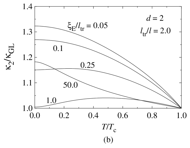
Figure 4: Temperature dependence of $\kappa_{2}/\kappa_{\rm GL}$ for an isotropic two-dimensional system in the extreme type-II case $\kappa_{\rm GL}\!=\!50$. (a) $l_{\rm tr}/l=1.0$; (b) $l_{\rm tr}/l=2.0$.

The above calculations are performed for an idealized spherical Fermi surface. However, real superconductors are often characterized by complicated Fermi surfaces. To see the dependence of $\kappa_{2}/\kappa_{\rm GL}$ on Fermi-surface structures, I have performed an isotropic two-dimensional calculation described in Sec. II.3. Figure 4 shows the results, where the parameters are the same as those in Fig. 1. The curves for $\xi_{\rm E}/l_{\rm tr}\!=\!50$ are almost the same as those in Fig. 1. Thus, in the dirty limit, we have a universal curve which depends neither on detailed Fermi-surface structures nor fine features of the impurity scattering. As the system becomes cleaner, however, differences due to the two factors emerge eventually. In fact, we observe that each curve for $\xi_{\rm E}/l_{\rm tr}\!\lesssim\!1.0$ in Fig. 4 deviates far less from $1$ than the corresponding one in Fig. 1, and the temperature dependence is also weaker. Another point to be mentioned is that, even for $\xi_{\rm E}/l_{\rm tr}\!=\!0.05$, we see no trace of divergence as $T\!\rightarrow\!0$. Indeed, a closer examination of the analytic results by Maki and TsuzukiMT65 and EilenbergerEilenberger67 enables us to realize that it is the region $\theta\!\sim\!0$ in three dimensions which is responsible for the divergence of $\kappa_{2}$. Thus, we may conclude that $\kappa_{2}$ in two dimensions remains finite even in the clean limit as $T\!\rightarrow\!0$. In general, $\kappa_{2}$ will remain finite if the relevant Fermi surface does not close along the direction of the magnetic field.

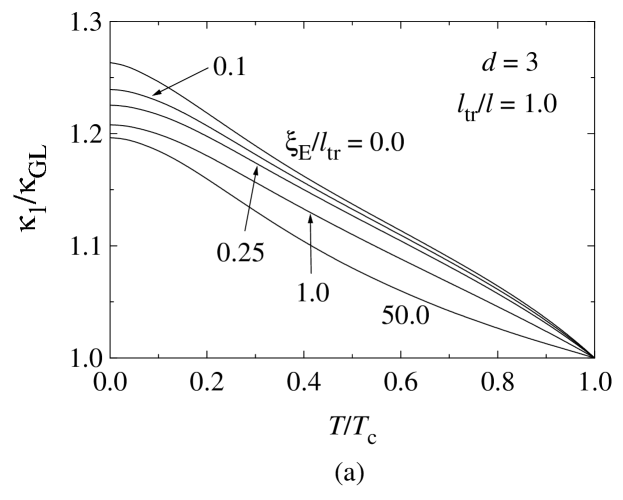
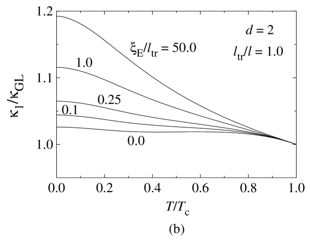
Figure 5: Temperature dependence of $\kappa_{1}/\kappa_{\rm GL}$ for several values of $\xi_{\rm E}/l_{\rm tr}$ with $l_{\rm tr}/l=1.0$. (a) $d\!=\!3$ ; (b) $d\!=\!2$.

III.3 Results for $\kappa_{1}$

The Maki parameter $\kappa_{1}$ is defined byMaki64

$$\kappa_{1}\equiv{H_{c2}}/{\sqrt{2}H_{c}}\,,$$ (53)

where $H_{c}\!=\!H_{c}(T)$ is the thermodynamic critical field. The preceding results for $\kappa_{2}$ suggest that $\kappa_{1}(T)/\kappa_{\rm GL}$ may also exhibit considerable dependence on detailed Fermi-surface structures.

Figure 5 compares $\kappa_{1}(T)/\kappa_{\rm GL}$ between two and three dimensions for $l_{\rm tr}/l\!=\!1.0$. The curves for $\xi_{\rm E}/l_{\rm tr}\!=\!50$ show almost the same behavior. As $\xi_{\rm E}/l_{\rm tr}$ becomes smaller, however, the two cases display a marked difference. Indeed, $\kappa_{1}(T)/\kappa_{\rm GL}$ is seen to increase (decrease) in three (two) dimensions as $\xi_{\rm E}/l_{\rm tr}\!\rightarrow\!0$.

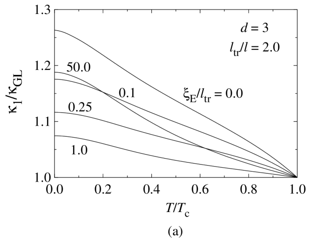
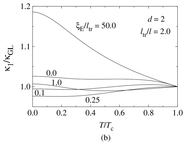
Figure 6: Temperature dependence of $\kappa_{1}/\kappa_{\rm GL}$ for several values of $\xi_{\rm E}/l_{\rm tr}$ with $l_{\rm tr}/l=2.0$. (a) $d\!=\!3$ ; (b) $d\!=\!2$.

Figure 6 shows curves of $\kappa_{1}(T)/\kappa_{\rm GL}$ in two and three dimensions for $l_{\rm tr}/l\!=\!2.0$. Again the $p$-wave impurity scattering is seen to lower the value of $\kappa_{1}/\kappa_{\rm GL}$, and also introduces non-monotonicity in $\kappa_{1}/\kappa_{\rm GL}$ as a function of $\xi_{\rm E}/l_{\rm tr}$. Especially in two dimensions for $\xi_{\rm E}/l_{\rm tr}\!=\!0.1$-$1.0$, $\kappa_{1}/\kappa_{\rm GL}$ becomes smaller than $1$ over finite temperature ranges, i.e., the emperical inequality $\kappa_{2}\!\geq\!\kappa_{1}\!\geq\!\kappa_{\rm GL}$ is not satisfied here, even without spin paramagnetism.Maki66

A substantial dependence of $H_{c2}$ on Fermi-surface structures may be realized more clearly by looking at the temperature dependence of the reduced critical field introduced by Helfand and Werthamer:HW66

$$h^{*}(t)\equiv\frac{H_{c2}(t)}{-dH_{c2}(t)/dt|_{t=1}}\,,$$ (54)

where $t\!\equiv T/T_{c}$. Figure 7 compares $h^{*}(t)$ between two and three dimensions for both the clean and dirty limits. The curves coincide in the dirty limit, whereas those in the clean limit show a marked quantitative difference. We also observe that $h^{*}(t)$ in two dimensions is a rather sensitive function of purity. A considerable reduction of $h^{*}_{d=2}(t)$ in the pure limit from $h^{*}_{d=3}(t)$ may be attributed to the pair breaking by supercurrent. This effect is more effective in two dimensions. Indeed, a point on the cylindrical Fermi surface is equivalent to a point on the equator of the spherical Fermi surface perpendicular to ${\bf H}$ where the pair breaking is most effective. This fact can be seen clearly in the polar-angle dependence of the density of states calculated by Brandt, Pesch, and Tewordt.BPT67 Put it another way, if the relevant Fermi surface does not have a closed orbit perpendicular to ${\bf H}$, the corresponding $h^{*}(t)$ in the clean limit will be enhanced over the prediction for the spherical Fermi surface.

A considerable reduction of $h^{*}(t)$ or $\kappa_{1}(t)$ in the presence of spin paramagnetism was established by Werthamer, Helfand, and Hohenberg,WHH66 and also by Maki.Maki66 The present results indicate unambiguously that the Fermi-surface structure is also an important factor for $h^{*}(t)$ in clean systems, as already noticed by Helfand and Werthamer,HW66 Hohenberg and Werthamer,HW67 and Werthamer and McMillan.WM67

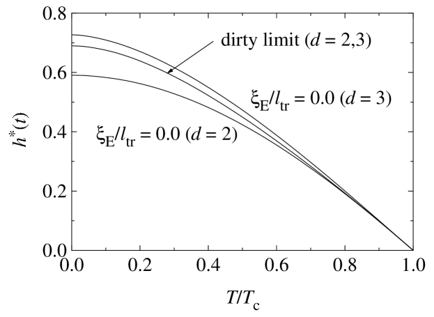
Figure 7: Temperature dependence of the reduced critical field $h^{*}(t)$ for the dirty limit of $d\!=\!2,3$ (mid curve) and the clean limit of $d\!=\!2$ (lower curve) and $d\!=\!3$ (upper curve).

III.4 Results for the pair potential

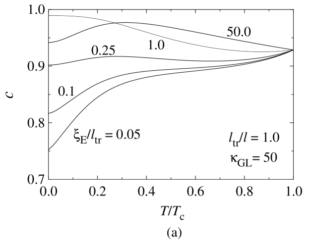
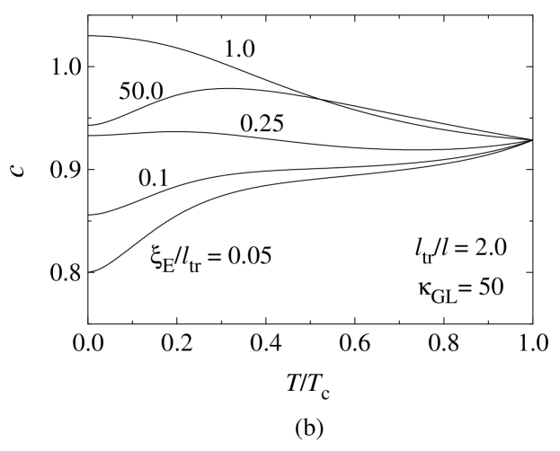
Figure 8: The coefficient $c(T)\!\equiv\!(1\!-\!B/H_{c2})^{1/2}\Delta(T)/\Delta_{0}(B,T)$ in the extreme type-II case $\kappa_{\rm GL}\!=\!50$ as a function of $T/T_{c}$ for several values of $\xi_{\rm E}/l_{\rm tr}$. (a) $l_{\rm tr}/l=1.0$ ; (b) $l_{\rm tr}/l=2.0$.

A quantity of fundamental importance is the coefficient $\Delta_{0}$, which is equal to the spatial average $\sqrt{\langle|\Delta({\bf r})|^{2}\rangle}$ of the pair potential and relevant to all thermodynamic and transport properties near $H_{c2}$. It is physically more meaningful to express it as a function of the real average field $B$ in the bulk instead of $H$. Equation (36) shows that $\Delta_{0}(B)$ is proportional to $(H_{c2}\!-\!B)^{1/2}$ near $H_{c2}$. I here express this $\Delta_{0}$ by using the energy gap $\Delta(T)$ at $B\!=\!0$ as

$$\Delta_{0}(B,T)=c(T)(1\!-\!B/H_{c2})^{1/2}\Delta(T)\,.$$ (55)

Then the coefficient $c(T)$ should be of the order of $1$.

Figure 8, calculated for the spherical Fermi surface, displays temperature dependence of $c(T)$ in an extreme type-II case of $\kappa_{\rm GL}\!=\!50$ for (a) $l_{\rm tr}/l\!=\!1.0$ and (b) $l_{\rm tr}/l\!=\!2.0$. Thus $c(T)\!\sim\!1$, as expected, having the same value $0.929$ at $T_{c}$. Differences among different $\xi_{\rm E}/l_{\rm tr}$ grow at lower temperatures, and $c(T)$ for $\xi_{\rm E}/l_{\rm tr}\!\lesssim\!0.1$ drops rapidly near $T\!=\!0$. Indeed, $c(T)$ in the clean limit for three dimensions is expected to reach $0$ as $T\!\rightarrow\!0$, corresponding to the divergence of $\kappa_{2}$. This also implies that the expansion in $\Delta({\bf r})$ near $H_{c2}$ is no longer valid in this limit.FH69 The curves in the dirty limit are the same between $l_{\rm tr}/l\!=\!1.0$ and $l_{\rm tr}/l\!=\!2.0$. For $\xi_{\rm E}/l_{\rm tr}\!\lesssim\!1.0$, however, each curve for $l_{\rm tr}/l\!=\!2.0$ at low temperatures has larger values than the corresponding one for $l_{\rm tr}/l\!=\!1.0$. Thus, finite $p$-wave scattering in clean systems tends to increase $c(T)$.

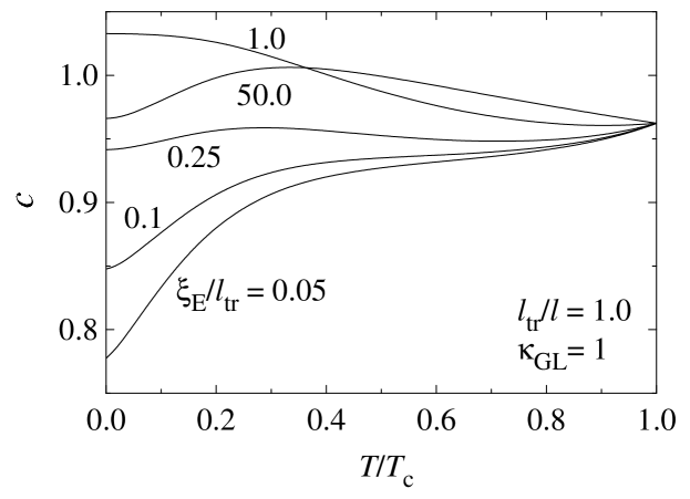
Figure 9: The coefficient $c(T)$ for $\kappa_{\rm GL}\!=\!1$ as a function of $T/T_{c}$ for several values of $\xi_{\rm E}/l_{\rm tr}$ with $l_{\rm tr}/l=1.0$.

The coefficient $c(T)$ also increases mildly as $\kappa_{\rm GL}$ becomes smaller, as realized by comparing Fig. 9 for $\kappa_{\rm GL}\!=\!1$ with Fig. 8(a) for $\kappa_{\rm GL}\!=\!50$.

Figure 10 plots results of the two-dimensional calculations performed with the same parameters as those in Fig. 8. The curves for the dirty limit are the same between two and three dimensions. As the system becomes cleaner, however, the coefficient $c(T)$ for two dimensions becomes larger than the corresponding one for three dimensions. Thus, for clean systems, we observe once again a considerable dependence of the coefficient $c(T)$ on Fermi-surface structures.

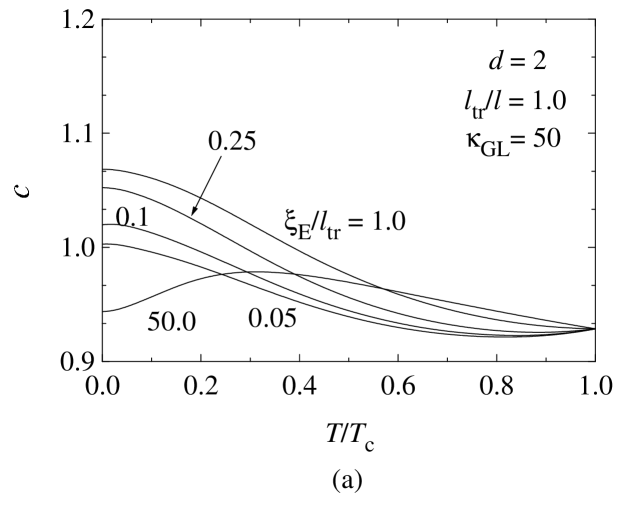
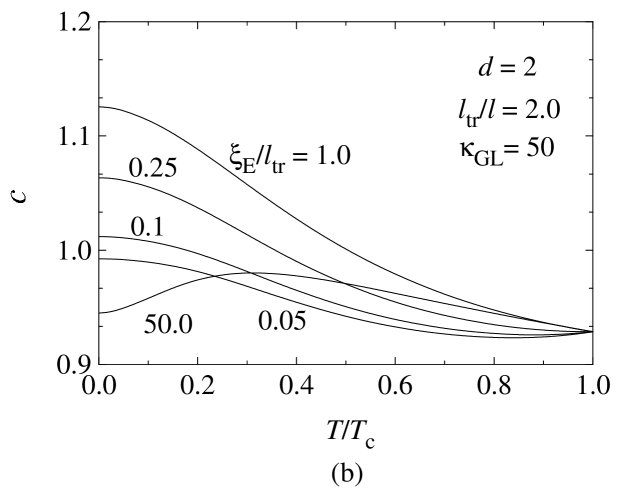
Figure 10: The coefficient $c(T)$ in two dimensions with $\kappa_{\rm GL}\!=\!50$ as a function of $T/T_{c}$ for several values of $\xi_{\rm E}/l_{\rm tr}$. (a) $l_{\rm tr}/l=1.0$ ; (b) $l_{\rm tr}/l=2.0$.

IV summary

This paper has presented revised calculations of the Maki parameters $\kappa_{1}$ and $\kappa_{2}$ as well as the spatial average $\langle|\Delta({\bf r})|^{2}\rangle$ near $H_{c2}$. Eilenberger’s results for $\kappa_{2}$ have been corrected appropriately, as described in Sec. II.8. The analytic expressions derived in Secs. II.5 and II.6 have been useful to carry out efficient calculations for both two and three dimensions with isotropic Fermi surfaces and arbitrary impurity concentrations. Thereby found are large quantitative differences of the parameters between two and three dimensions (except in the dirty limit where there are no differences between the two cases). For example, no trace of divergence in $\kappa_{2}(T\!\rightarrow\!0)$ is found for the clean limit in two dimensions.

The present results clearly indicates the necessity of considering detailed Fermi-surface structures from first-principle calculations for an quantitative understanding of the Maki parameters in clean superconductors. This was already recognized by Helfand and Werthamer,HW66 by Hohenberg and Werthamer,HW67 and also by Werthamer and McMillanWM67 when their strong-coupling calculation could not explain a large deviation of $\kappa_{1}/\kappa_{\rm GL}$ observed in pure niobiumMS65 ; FSS66 and vanadiumRK66 from the theoretical prediction of Helfand and Werthamer.HW66 Efforts have been made along this line to establish a realistic calculation of $\kappa_{1}$, or equivalently, $H_{c2}$.HW67 ; TN70 ; Mattheiss70 ; Teichler75 ; EP76 ; Butler80 ; YK80 ; PS87 ; RS90 ; Weber91 ; Langmann92 However, little progress seems to have been achieved with respect to $\kappa_{2}$.

The method developed here for $\kappa_{1}$ and $\kappa_{2}$ may be extended easily to include Fermi-surface structures and anisotropic pairings. Some of the necessary modifications are: (i) to use the general expansion (13a) with $N\!=\!{\rm even}$ for the pair potential, rather than Eq. (15); (ii) to use more convenient basisfunctions than ${\rm e}^{im\varphi}$ in Eq. (13b) for describing the ${\bf k}_{\rm F}$ dependence of $f(\varepsilon_{n},{\bf k}_{\rm F},{\bf r})$, such as the Fermi-surface harmonics of Allen.Allen76 ; BA76 ; Allen78 ; AM82 The corresponding matrix $\tilde{\cal M}$ in Eqs. (17a) and (17b) is no longer tridiagonal, but may be inverted rather easily with present high-speed computers.

Appendix A Derivation of Eq. (4)

To obtain Eq. (4), let us start from Eilenberger’s free-energy functionalEilenberger68 per unit volume with $B$ chosen as an independent variable instead of $H$. It is given in units of $N(0)\Delta(0)^{2}$ as

$$\frac{F(B)}{V}=\frac{1}{V}\int\!d{\bf r}\biggl{\{}\frac{\kappa_{0}^{2}}{2}\left[B^{2}\!+\!({\bm{\nabla}}\!\times\!\tilde{\bf A})^{2}\right]+|\Delta({\bf r})|^{2}\ln\frac{T}{T_{c}}$$

$$+2\pi T\sum_{n=0}^{\infty}\left[\frac{|\Delta({\bf r})|^{2}}{\varepsilon_{n}}-\langle I(\varepsilon_{n},{\bf k}_{\rm F},{\bf r})\rangle\right]\biggr{\}}\,,\,\,\,\,\,\,\,\,\,\,$$ (56)

where $I$ is defined by

$$I\equiv\Delta^{\!*}f\!+\!\Delta f^{\dagger}+2\varepsilon_{n}(g\!-\!1)+\frac{f\langle f^{\dagger}\rangle\!+\!\langle f\rangle f^{\dagger}}{4\tau}+\frac{g\langle g\rangle\!-\!1}{2\tau}$$

$$\hskip 8.53581pt+(g\!-\!1)\hat{\bf v}\cdot\frac{f^{\dagger}({\bm{\nabla}}\!-\!i{\bf A})f-f({\bm{\nabla}}\!+\!i{\bf A})f^{\dagger}}{2ff^{\dagger}}\,.$$ (57)

The functional derivatives of Eq. (56) with respect to $f^{\dagger}$, $\Delta$, and $\bf A$ lead to Eqs. (2a)-(2c), respectively. The last term in Eq. (57) is slightly different from the original functional of Eilenberger where $g\hat{\bf v}$ appears in place of $(g\!-\!1)\hat{\bf v}$.Eilenberger68 Although it does not change Eq. (2) at all, it is found numerically that the modification is necessary for $F$ to have its absolute minimum with respect to $\Delta$, $\bf A$, and $f\!=\!f(\Delta,{\bf A})$ satisfying Eq. (2a), as anticipated by Eilenberger.Eilenberger68 It should be noted that Pesch and KramerPK74 also adopted Eq. (56) as a basis for their numerical calculations. More recently, Endres and RainerER03 performed a numerical calculation of the free energy for both an SN contact and a single vortex based on Eq. (56), and compared the results with those from three free-energy functionals obtained from the Luttinger-Ward functional. They found numerical agreements among the values from the four different expressions.

Following Doria, Gubernatis, and Rainer,DGR89 I now rewrite the right-hand side of Eq. (56) in terms of

$$\begin{array}[]{c}\vspace{2mm}{\bf r}^{\prime}\!\equiv{\bf r}/\lambda,\hskip 8.53581ptB_{\lambda}\!\equiv\!\lambda^{2}B,\hskip 8.53581pt\tilde{\bf A}_{\lambda}({\bf r}^{\prime})\!\equiv\!\lambda\tilde{\bf A}(\lambda{\bf r}^{\prime}),\\ \Delta_{\lambda}({\bf r}^{\prime})\!\equiv\!\Delta(\lambda{\bf r}^{\prime}),\hskip 8.53581ptf_{\lambda}(\varepsilon_{n},{\bf k}_{\rm F},{\bf r}^{\prime})\equiv f(\varepsilon_{n},{\bf k}_{\rm F},\lambda{\bf r}^{\prime}).\end{array}$$ (60)

I then differentiate the resulting expression with respect to $\lambda$ and put $\lambda\!=\!1$. Since the procedure (60) does not change the value of $F/V$, we have $\frac{\partial}{\partial\lambda}(F/V)|_{\lambda=1}\!=\!0$ from the left-hand side. As for the right-hand side, the only implicit dependence to be considered is the one from $B_{\lambda}$; those from $f_{\lambda}$, $\Delta_{\lambda}$, and $\tilde{\bf A}_{\lambda}$ can be neglected due to the stationarity of Eq. (2). We thereby obtain

$$0=\left.\frac{\partial(F/V)}{\partial B_{\lambda}}\frac{\partial B_{\lambda}}{\partial\lambda}\right|_{\lambda=1}-2\kappa_{0}^{2}B^{2}-\frac{2\kappa_{0}^{2}}{V}\int\!d{\bf r}\,({\bm{\nabla}}\!\times\!\tilde{\bf A})^{2}$$

$$-\frac{\pi T}{V}\!\sum_{n=0}^{\infty}\int\!d{\bf r}\left<\!\frac{f^{\dagger}\hat{\bf v}\!\cdot\!({\bm{\nabla}}\!-\!i{\bf A})f\!-\!f\hat{\bf v}\!\cdot\!({\bm{\nabla}}\!+\!i{\bf A})f^{\dagger}}{1+g}\!\right>.$$

Using the thermodynamic relation $\frac{\partial(F/V)}{\partial B_{\lambda}}|_{\lambda=1}=\kappa_{0}^{2}H$ in the present units, we arrive at Eq. (4).

Appendix B Extension to the case with $p$-wave impurity scattering

In the presence of $p$-wave impurity scattering, Eq. (2a) is replaced by

$$\left[\varepsilon_{n}+\frac{\langle g\rangle}{2\tau}+\frac{d\,\hat{\bf k}\!\cdot\!\langle\hat{\bf k}^{\prime}g\rangle}{2\tau_{1}}+\frac{\hat{\bf v}}{2}\!\cdot\!\left({\bm{\nabla}}-i{\bf A}\right)\right]f$$

$$=\left(\Delta+\frac{\langle f\rangle}{2\tau}+\frac{d\,\hat{\bf k}\!\cdot\!\langle\hat{\bf k}^{\prime}f\rangle}{2\tau_{1}}\right)g\,,$$ (62)

where $\langle\hat{\bf k}^{\prime}g\rangle\!\equiv\!\langle\hat{\bf k}^{\prime}g(\varepsilon_{n},{\bf k}_{\rm F}^{\prime},{\bf r})\rangle$, for example, and $d\!=\!2,3$ is the dimension of the system. This brings additional terms on the right-hand side of Eqs. (17a) and (17b) as

$$\sum_{N^{\prime}}\tilde{\cal M}_{NN^{\prime}}\tilde{f}_{N^{\prime}}^{(1)} =\delta_{N0}\left(1+\frac{\langle\tilde{f}_{0}^{(1)}\rangle}{2\tau}+\frac{d\cos\theta\,\langle\tilde{f}_{0}^{(1)}\!\cos\theta^{\prime}\rangle}{2\tau_{1}}\right)$$ (63)

$$+\delta_{N1}\frac{d\sin\theta\,\langle\tilde{f}_{1}^{(1)}\!\sin\theta^{\prime}\rangle}{4\tau_{1}}$$

$$\sum_{N^{\prime}}\tilde{\cal M}_{NN^{\prime}}\tilde{f}_{N^{\prime}}^{(3)}=\delta_{N0}\left(\frac{\langle\tilde{f}_{0}^{(3)}\rangle}{2\tau}+\frac{d\cos\theta\,\langle\tilde{f}_{0}^{(3)}\!\cos\theta^{\prime}\rangle}{2\tau_{1}}\right)$$

$$\hskip 28.45274pt+\delta_{N1}\frac{d\sin\theta\,\langle\tilde{f}_{1}^{(3)}\!\sin\theta^{\prime}\rangle}{4\tau_{1}}+J_{N}^{(3)}+J_{N}^{(A)}\,,$$ (64)

where $J_{N}^{(A)}$ is given by Eq. (19c), and $J_{N}^{(3)}$ is defined instead of Eq. (19b) by

$$J_{N}^{(3)}\equiv-\frac{1}{2}\!\sum_{N^{\prime}}(-1)^{N^{\prime}}I_{NN^{\prime}N+N^{\prime}0}^{(4)}\,\tilde{f}_{N^{\prime}}^{(1)}\tilde{f}_{N+N^{\prime}}^{(1)}$$

$$\hskip 56.9055pt\times\biggl{(}\!1+\frac{\langle\tilde{f}_{0}^{(1)}\rangle}{2\tau}+\frac{d\cos\theta\,\langle\tilde{f}_{0}^{(1)}\!\cos\theta^{\prime}\rangle}{2\tau_{1}}\!\biggr{)}$$

$$+\frac{1}{4}\sum_{N^{\prime}}(-1)^{N^{\prime}}I_{NN^{\prime}N^{\prime}N}^{(4)}\,$$

$$\hskip 28.45274pt\times\left(\frac{\langle\tilde{f}_{N^{\prime}}^{(1)}\tilde{f}_{N^{\prime}}^{(1)}\rangle}{\tau}+\frac{d\cos\theta\,\langle\tilde{f}_{N^{\prime}}^{(1)}\tilde{f}_{N^{\prime}}^{(1)}\!\cos\theta^{\prime}\rangle}{\tau_{1}}\right)\tilde{f}_{N}^{(1)}$$

$$+\frac{d\sin\theta}{8\tau_{1}}\sum_{N^{\prime}}(-1)^{N^{\prime}}\biggl{[}-I_{NN^{\prime}N+N^{\prime}-11}^{(4)}\,\tilde{f}_{N^{\prime}}^{(1)}\tilde{f}_{N+N^{\prime}-1}^{(1)}$$

$$\hskip 8.53581pt\times\,\langle\tilde{f}_{1}^{(1)}\!\sin\theta^{\prime}\rangle+I_{NN^{\prime}N^{\prime}-1N+1}^{(4)}\,\langle\tilde{f}_{N^{\prime}}^{(1)}\tilde{f}_{N^{\prime}-1}^{(1)}\!\sin\theta^{\prime}\rangle\tilde{f}_{N+1}^{(1)}$$

$$\hskip 8.53581pt+I_{NN^{\prime}N^{\prime}+1N-1}^{(4)}\,\langle\tilde{f}_{N^{\prime}}^{(1)}\tilde{f}_{N^{\prime}+1}^{(1)}\!\sin\theta^{\prime}\rangle\tilde{f}_{N-1}^{(1)}\biggr{]}\,.$$ (65)

Equation (63) can be solved in the same way as Eq. (26) to yield

$$\tilde{f}_{N}^{(1)}={\tilde{K}^{0}_{N}}\left(1+\frac{\langle\tilde{f}_{0}^{(1)}\rangle}{2\tau}+\frac{d\cos\theta\,\langle\tilde{f}_{0}^{(1)}\!\cos\theta^{\prime}\rangle}{2\tau_{1}}\right)$$

$$+{\tilde{K}^{1}_{N}}\frac{d\sin\theta\,\langle\tilde{f}_{1}^{(1)}\!\sin\theta^{\prime}\rangle}{4\tau_{1}}\,.$$ (66)

From Eq. (66), we obtain self-consistent equations for $\langle\tilde{f}_{0}^{(1)}\rangle$, $\langle\tilde{f}_{0}^{(1)}\!\cos\theta\rangle$, and $\langle\tilde{f}_{1}^{(1)}\!\sin\theta\rangle$ as

$${\cal K}\left[\begin{array}[]{c}\vspace{1mm}\langle\tilde{f}_{0}^{(1)}\rangle\\ \vspace{1mm}\langle\tilde{f}_{0}^{(1)}\!\cos\theta\rangle\\ \langle\tilde{f}_{1}^{(1)}\!\sin\theta\rangle\end{array}\right]=\left[\begin{array}[]{c}\vspace{2mm}\langle\tilde{K}_{0}^{0}\rangle\\ \vspace{2mm}\langle\tilde{K}_{0}^{0}\!\cos\theta\rangle\\ \langle\tilde{K}_{1}^{0}\!\sin\theta\rangle\end{array}\right],$$ (73)

where the matrix ${\cal K}$ is defined by

$${\cal K}\equiv\left[\!\begin{array}[]{ccc}\vspace{2mm}\displaystyle 1\!-\!\frac{\langle\tilde{K}_{0}^{0}\rangle}{2\tau}\!&\!\displaystyle-\frac{d\langle\tilde{K}_{0}^{0}\!\cos\theta\rangle}{2\tau_{1}}\!&\!\displaystyle\frac{d\langle\tilde{K}_{1}^{0}\!\sin\theta\rangle}{4\tau_{1}}\\ \vspace{2mm}\displaystyle-\frac{\langle\tilde{K}_{0}^{0}\!\cos\theta\rangle}{2\tau}\!&\!\displaystyle 1\!-\!\frac{d\langle\tilde{K}_{0}^{0}\!\cos^{2}\theta\rangle}{2\tau_{1}}\!&\!\displaystyle\frac{d\langle\tilde{K}_{1}^{0}\!\sin 2\theta\rangle}{8\tau_{1}}\\ \\ \displaystyle-\frac{\langle\tilde{K}_{1}^{0}\!\sin\theta\rangle}{2\tau}\!&\!\displaystyle-\frac{d\langle\tilde{K}_{1}^{0}\!\sin 2\theta\rangle}{4\tau_{1}}\!&\!\displaystyle 1\!-\!\frac{d\langle\tilde{K}_{1}^{1}\!\sin^{2}\theta\rangle}{4\tau_{1}}\end{array}\!\right].$$ (74)

Noting $K_{N^{\prime}}^{N}\!=\!K_{N^{\prime}}^{N}(\tilde{\varepsilon}_{n},\beta)$ as seen from Eqs. (41)-(43) with $\beta$ defined in Eq. (9), we immediately realize that $\langle\tilde{K}_{0}^{0}\!\cos\theta\rangle\!=\!0$ in Eq. (73) and ${\cal K}_{2j}\!=\!{\cal K}_{j2}\!=\!0$ for $j\!=\!1,3$ in Eq. (74). Thus, Eq. (73) can be solved easily with $\langle\tilde{f}_{0}^{(1)}\!\cos\theta\rangle\!=\!0$. Substituting the resulting expressions of $\langle\tilde{f}_{0}^{(1)}\rangle$ and $\langle\tilde{f}_{1}^{(1)}\!\sin\theta\rangle$ into Eq. (66), we obtain

$$\tilde{f}_{N}^{(1)}$$

$$=\frac{\bigl{(}1\!-\!\frac{d}{4\tau_{1}}{\langle\tilde{K}_{1}^{1}\!\sin^{2}\theta^{\prime}\rangle}\bigr{)}\tilde{K}^{0}_{N}+\frac{d}{4\tau_{1}}{\langle\tilde{K}_{1}^{0}\!\sin\theta^{\prime}\rangle\tilde{K}^{1}_{N}\sin\theta}}{\bigl{(}1\!-\!\frac{1}{2\tau}\langle\tilde{K}_{0}^{0}\rangle\bigr{)}\bigl{(}1\!-\!\frac{d}{4\tau_{1}}\langle\tilde{K}_{1}^{1}\!\sin^{2}\theta^{\prime}\rangle\bigr{)}+\frac{d}{8\tau\tau_{1}}\langle\tilde{K}_{1}^{0}\!\sin\theta^{\prime}\rangle^{2}}\,.$$

(75)

Equation (65) is also simplified into

$$J_{N}^{(3)}\equiv-\frac{1}{2}\!\sum_{N^{\prime}}(-1)^{N^{\prime}}I_{NN^{\prime}N+N^{\prime}0}^{(4)}\,\tilde{f}_{N^{\prime}}^{(1)}\tilde{f}_{N+N^{\prime}}^{(1)}\biggl{(}\!1+\frac{\langle\tilde{f}_{0}^{(1)}\rangle}{2\tau}\!\biggr{)}$$

$$+\frac{1}{4\tau}\sum_{N^{\prime}}(-1)^{N^{\prime}}I_{NN^{\prime}N^{\prime}N}^{(4)}\,\langle\tilde{f}_{N^{\prime}}^{(1)}\tilde{f}_{N^{\prime}}^{(1)}\rangle\tilde{f}_{N}^{(1)}$$

$$+\frac{d\sin\theta}{8\tau_{1}}\sum_{N^{\prime}}(-1)^{N^{\prime}}\biggl{[}-I_{NN^{\prime}N+N^{\prime}-11}^{(4)}\,\tilde{f}_{N^{\prime}}^{(1)}\tilde{f}_{N+N^{\prime}-1}^{(1)}$$

$$\hskip 8.53581pt\times\,\langle\tilde{f}_{1}^{(1)}\!\sin\theta^{\prime}\rangle+I_{NN^{\prime}N^{\prime}-1N+1}^{(4)}\,\langle\tilde{f}_{N^{\prime}}^{(1)}\tilde{f}_{N^{\prime}-1}^{(1)}\!\sin\theta^{\prime}\rangle\tilde{f}_{N+1}^{(1)}$$

$$\hskip 8.53581pt+I_{NN^{\prime}N^{\prime}+1N-1}^{(4)}\,\langle\tilde{f}_{N^{\prime}}^{(1)}\tilde{f}_{N^{\prime}+1}^{(1)}\!\sin\theta^{\prime}\rangle\tilde{f}_{N-1}^{(1)}\biggr{]}\,.$$ (76)

Equation (64) can be treated similarly to obtain $\langle\tilde{f}_{0}^{(3)}\rangle$ which appears in Eq. (17c). Then a straightforward calculation leads to the same expression (28) for $\langle\tilde{f}_{0}^{(3)}\rangle$ with $\tilde{f}^{(1)}_{N}$ and $J^{(3)}_{N}$ replaced by Eqs. (75) and (76), respectively. Another relevant quantity in Eq. (17c) is $\langle\tilde{f}_{0}^{(1)^{\prime}}\rangle$, as seen from Eq. (30). Differentiating Eq. (63) with respect to $B$ and solving the resulting equation self-consistently, we also obtain Eq. (32) for $\langle\tilde{f}_{0}^{(1)^{\prime}}\rangle$ with $\tilde{f}^{(1)}_{N}$ in Eq. (19a) replaced by Eqs. (75).

It hence follows that Eqs. (34) and (35) remains the same in the presence of the $p$-wave impurity scattering with $\tilde{f}^{(1)}_{N}$ and $J^{(3)}_{N}$ replaced by Eqs. (75) and (76), respectively.

References

- (1) L.P. Gor’kov, Zh. Eksp. Teor. Fiz. 37, 833 (1959); Sov. Phys. JETP 10, 593 (1960).
- (2) K. Maki, Physics 1, 21 (1964).
- (3) P.G. de Gennes, Phys. Condens. Matter 3, 79 (1965).
- (4) L. Tewordt, Z. Phys. 184, 319 (1965).
- (5) E. Helfand and N.R. Werthamer, Phys. Rev. Lett. 13, 686 (1964); Phys. Rev. 147, 288 (1966).
- (6) N.R. Werthamer, E. Helfand, and P.C. Hohenberg, Phys. Rev. 147, 295 (1966).
- (7) G. Eilenberger, Z. Phys. 190, 142 (1966).
- (8) K. Maki and T. Tsuzuki, Phys. Rev. 139, A868 (1965).
- (9) L. Neumann and L. Tewordt, Z. Phys. 191, 73 (1966).
- (10) C. Caroli, M. Cyrot, and P.G. de Gennes, Solid State Commun. 4, 17 (1966).
- (11) K. Maki, Phys. Rev. 148, 362 (1966).
- (12) G. Eilenberger, Phys. Rev. 153, 584 (1967). Equation numbers (2.7) and (2.8) for the last two equations of Sec. II are missing, although referred in the manuscript.
- (13) V.L. Ginzburg and L.D. Landau, Zh. Eksp. Teor. Fiz. 20, 1064 (1950).
- (14) For a review on the whole topic, see, A.L. Fetter and P.C. Hohenberg, in Superconductivity, edited by R.D. Parks (Dekker, NY, 1969), Vol. 2, p. 817; B. Serin, ibid. Vol. 2, p. 925.
- (15) G. Eilenberger, Z. Phys. 214, 195 (1968); I consider positively charged particles following the convention. The case of electrons can be obtained directly by , i.e., reversing the magnetic-field direction.
- (16) J.W. Serene and D. Rainer, Phys. Rep. 101, 221 (1983).
- (17) L.P. Gor’kov, Zh. Eksp. Teor. Fiz. 37, 1407 (1959); Sov. Phys. JETP 10, 998 (1960).
- (18) Yu.N. Ovchinnikov and E.H. Brandt, phys. stat. sol. (b) 67, 301 (1975). Although they calculated using Eilenberger equations, their main interest was directed towards nonlinearity of magnetization near for clean superconductors at low temperatures.
- (19) G. Eilenberger: Z. Phys. 180 32, (1964).
- (20) G. Lasher: Phys. Rev. 140 A523, (1965).
- (21) P.M. Marcus, in Proceedings of the Tenth International Conference on Low Temperature Physics, ed. M.P. Malkov et al. (Viniti, Moscow, 1967) Vol. IIA, p. 345.
- (22) E.H. Brandt, Phys. Stat. Sol. B 51 345, (1972); Phys. Rev. Lett. 78, 2208 (1997).
- (23) M.M. Doria, J.E. Gubernatis and D. Rainer, Phys. Rev. B 41, 6335 (1990).
- (24) T. Kita, J. Phys. Soc. Jpn. 67, 2067 (1998).
- (25) M.M. Doria, J.E. Gubernatis and D. Rainer, Phys. Rev. B 39, 9573 (1989).
- (26) A.A. Abrikosov: Zh. Eksp. Teor. Fiz. 32, 1442 (1957) [Sov. Phys. JETP 5, 1174 (1957)].
- (27) A.C. Aitken, Determinants and matrices (Interscience, New York, 1956).
- (28) T. Kita, J. Phys. Soc. Jpn. 67, 2075 (1998).
- (29) U. Brandt, W. Pesch, and L. Tewordt, Z. Phys. 201, 209 (1967).
- (30) P.C. Hohenberg and N.R. Werthamer, Phys. Rev. 153, 493 (1967).
- (31) N.R. Werthamer and W.L. McMillan, Phys. Rev. 158, 415 (1967).
- (32) T. McConville and B. Serin, Phys. Rev. 140, A1169 (1965).
- (33) D.K. Finnemore, T.F. Stromberg, and C.A. Swenson, Phys. Rev. 149, 231 (1966).
- (34) R. Radebaugh and P.H. Keesom, Phys. Rev. 149, 217 (1966).
- (35) K. Takanaka and T. Nagashima, Prog. Theor. Phys. 43, 18 (1970).
- (36) L.F. Mattheiss, Phys. Rev. B 1, 373 (1970).
- (37) H. Teichler, Phys. Status Solidi B 69, 501 (1975).
- (38) P. Entel and M. Peter, J. Low Temp. Phys. 22, 613 (1976).
- (39) W.H. Butler, Phys. Rev. Lett. 44, 1516 (1980).
- (40) D.W. Youngner and R.A. Klemm, Phys. Rev. B 21, 3890 (1980).
- (41) M. Prohammer and E. Schachinger, Phys. Rev. B 36, 8353 (1987).
- (42) C.T. Rieck and K. Scharnberg, Physica B 163, 670 (1990).
- (43) H.W. Weber, E. Seidl, C. Laa, E. Schachinger, M. Prohammer, A. Junod, and D. Eckert, Phys. Rev. B 44, 7585 (1991).
- (44) E. Langmann, Phys. Rev. B 46, 9104 (1992).
- (45) P. B. Allen, Phys. Rev. B 13, 1416 (1976).
- (46) W.H. Butler and P.B. Allen, in Superconductivity in d- and f-Band Metals, edited by D.H. Douglass (Plenum, New York, 1976), p. 73.
- (47) P.B. Allen, Phys. Rev. B 17, 3725 (1978).
- (48) P.B. Allen and B. Mitrovich, in Solid State Physics, edited by F. Seitz, D. Turnbull, and H. Ehrenreich (Academic, New York, 1982), Vol. 37, p. 1.
- (49) W. Pesch and L. Kramer, J. Low Temp. Phys. 15, 367 (1974).
- (50) M. Endres and D. Rainer, private communication.