Ballistic Localization in Quasi-1D Waveguides with Rough Surfaces

Abstract

Structure of eigenstates in a periodic quasi-1D waveguide with a rough surface is studied both analytically and numerically. We have found a large number of ”regular” eigenstates for any high energy. They result in a very slow convergence to the classical limit in which the eigenstates are expected to be completely ergodic. As a consequence, localization properties of eigenstates originated from unperturbed transverse channels with low indexes, are strongly localized (delocalized) in the momentum (coordinate) representation. These eigenstates were found to have a quite unexpeted form that manifests a kind of ”repulsion” from the rough surface. Our results indicate that standard statistical approaches for ballistic localization in such waveguides seem to be unappropriate.

In the past decade much attention has been paid to statistical properties of eigenstates of closed disordered systems. As a result, to date practically everything is known for quasi-1D systems with ”bulk disorder”. The success is mainly related to the developments of the non-linear $\sigma$ model (see, e.g. [1] and references therein). One of the most important results is that the statistical properties of such systems are essentially determined by one characteristic length only, known as the localization length of eigenstates. This fact is entirely due to a strong mixing between transverse channels resulting from bulk scattering and leading to a diffusive character of transport.

A much more difficult situation was found to occur for the models with surface scattering when the disorder is due to a surface roughness. In quasi-1D geometry such models are closely related to optical/microwave waveguides and have many physical applications in different fields [2]. The main problem in the rigorous treatment of this kind of systems is in the ballistic character of the scattering which has weaker statistical properties in comparison with diffusive scattering. Progress in this direction is related to recent developments of the ”ballistic sigma-model”, however, the problem is still far from being solved (see discussion and references in [3]).

As was recently shown in a number of numerical studies [4, 5], the transport in quasi-1D waveguides with rough surfaces is highly non-isotropic in channel space. Specifically, the transport through such waveguides strongly depends on the incident angle of incoming wave. In particular, the transmission coefficient smoothly decreases with an increase of the angle, since characterictic lengths for backscattering are different for different channels [5].

To understand generic features of surface disordered quasi-1D systems, in this Letter we perform a detailed study of the structure of eigenstates of a 2D quantum billiard (or waveguide). We consider billiards which are periodic in the longitudinal coordinate $x$, and with Dirichlet boundary conditions on the low, $y=0$, and upper, $y=d+a\xi(x)$, surfaces with $\xi(x+b)=\xi(x)$ and $\left<\xi(x)\right>=0$. Here the angular brackets stand for the average over one period $b$ (or, in the case of a random profile, over different realizations of $\xi(x)$).

Our main interest is in the study of the structure of eigenstates of this billiard in dependence on their energy and model parameters. For this we use the technique that transforms the Hamiltonian $\hat{H}=\frac{1}{2m_{e}}(\hat{P}_{x}^{2}+\hat{P}_{y}^{2})$ for a free particle inside the billiard with the above boundaries, to a new Hamiltonian which incorporates surface scattering effects into effective interaction potential. This can be achieved by the transformation to new canonical coordinates, $u=x;\,\,\,v=\frac{y}{1+\epsilon\xi(x)}$ with $\epsilon=a/d$. As a result, the boundary conditions for new wave function are trivial: $\Phi(u,v)=0$ at $v=0$ and $v=d$ (see details in [6])

In the new variables the Hamiltonian gets [6],

$$\hat{H}=-\frac{\hbar^{2}}{2m_{e}}\left(\frac{\partial^{2}}{\partial u^{2}}+h_{1}\frac{\partial^{2}}{\partial v^{2}}+h_{2}\frac{\partial^{2}}{\partial u\partial v}+h_{3}\frac{\partial}{\partial v}\right),$$ (1)

where

$$\begin{array}[]{ll}h_{1}=\frac{1+\epsilon^{2}v^{2}\xi_{u}^{2}}{(1+\epsilon\xi)^{2}},\,\,\,\,h_{2}=\frac{-2\epsilon v\xi_{u}}{1+\epsilon\xi},\,\,\,h_{3}=\frac{-\epsilon v\xi_{uu}}{1+\epsilon\xi}+\frac{2v\epsilon^{2}\xi_{u}^{2}}{(1+\epsilon\xi)^{2}},\end{array}$$ (2)

and $\xi_{u}=\partial\xi/\partial u,\,\xi_{uu}=\partial^{2}\xi/\partial u^{2}$.

One can write the Hamiltonian in the following form,

$$\hat{H}=\hat{H}^{0}+\hat{V}(u,v,\hat{P}_{u},\hat{P}_{v})\,;\,\,\,\,\,\hat{H}^{0}=\frac{1}{2m_{e}}(\hat{P}_{u}^{2}+\hat{P}_{v}^{2})$$ (3)

where $\hat{P}_{u}$ and $\hat{P}_{v}$ are the new canonical momenta. In this way, the ”unperturbed” Hamiltonian $\hat{H}^{0}$ descibes free motion of two ”particles” inside a billiard with flat boundaries, $y=0,\,\,\,y=d$, and $\hat{V}$ stands for an effective “interaction” between the “particles”. Such a representation turns out to be very convenient for the study of chaotic properties of our model, since one can use the tools and concepts developed in the theory of interacting particles (see [7] and references therein).

This model has been thoroughly studied in Refs.[6, 8, 9, 10, 11, 12] for the specific case $\xi(x)=\cos(2\pi x/b)$. The main interest was in the properties of energy spectrum [6, 10], and in the quantum-classical correspondence for the shape of eigenfunctions (SEF) and local density of states (LDOS) [8, 11]. In particular, it was shown that for highly excited states the global properties of the SEF and LDOS in the quantum model (3) are similar to those described by the equations of motion for a classical particle moving inside the billiard. On the other hand, quite strong quantum effects have been revealed for individual eigenstates in a deep semiclassical region [11].

Below we address the case of a rough surface $\xi(x)=\sum_{k=1}^{N_{T}}A_{k}\cos(2\pi kx/b)$, focusing on the properties of eigenstates. The surface is modeled by a large sum of harmonics with randomly distributed amplitudes $A_{k}$. With an increase of $N_{T}$ the degree of complexity of $\xi(x)$ increases and for a large $N_{T}\gtrsim 100$ the surface can be treated as the random one.

Since the Hamiltonian (3) is periodic in $u=x$, the eigenstates are Bloch states and the solution of the Schrödinger equation can be written in the form $\psi_{E}(u,v)=\exp(i\chi)\,\psi_{\chi}(u,v)$, with $\psi_{\chi}(u+2\pi/b,v)=\psi_{\chi}(u,v)$. Here the Bloch wave vector $\chi(E)$ is in the first Brillouin band, ($-\frac{\pi}{b}\leq\chi\leq\frac{\pi}{b})$. By expanding $\psi_{\chi}(u,v)$ in the basis of $\hat{H}_{0}$, the $\alpha$-th eigenstate of energy $E^{\alpha}(\chi)$ can be written as

$$\psi^{\alpha}(u,v;\chi)=\sum_{m=1}^{\infty}\sum_{n=-\infty}^{\infty}C_{mn}^{\alpha}(\chi)\phi_{mn}^{\chi}(u,v),$$ (4)

where $\phi_{mn}^{\chi}(u,v)\,=\pi^{-1/2}g^{-1/4}\sin(m\pi v/d)\,\exp\{i(\chi+2\pi n/b)u\}$. The factor $g=[1+\epsilon\xi(u)]^{2}$ arises from the orthonormality condition in the curvilinear coordinates $(u,v)$ (see details in [6]).

In the ”unperturbed” basis defined by $\hat{H}^{0}$, the matrix elements of the ”interaction” $\hat{V}(u,v,\hat{P}_{u},\hat{P}_{v})$ can be written explicitly for any profile $\xi(x)$ [11]. This fact is very useful in the study of the dependence of the properties of eigenstates on the form of profile.

The eigenvalues of $\hat{H}^{0}$ are given by the expression,

$$E^{(0)}_{n,m}(\chi)=\frac{\hbar^{2}}{2m_{e}}\left[\left(\chi+\frac{2\pi}{b}n\right)^{2}+\left(\frac{m\pi}{d}\right)^{2}\right].$$ (5)

In numerical simulations we have to make a cutoff for the values of $m$ and $n$ in the expansion (4). Our main results refer to the ranges, $1\leq m\leq M_{max}$ and $|n|\leq N_{max}$ with $N_{max}=32\,,M_{max}=62$, for which the total size of the Hamiltonian matrix is $L=(2N_{max}+1)M_{max}=4030$. Since the statistical properties of eigenstates do not depend on a specific value of the Bloch index $\chi$ inside the band [10], we fix it to $\chi=0.1\pi/b$.

One natural representation of the Hamiltonian matrix $H_{l,l^{\prime}}(\chi)=<l\mid\hat{H}\mid l^{\prime}>_{\chi}$ is the so-called ”channel representation” for which one fixes the values of $n$ starting from the lowest one, $n=-N_{max}$, with the run over $m$ for each $n$. In this way the matrix has a block structure that manifests peculiarities of the interaction between different channels specified by the index $m$. For our purpose, however, to analyze the properties of the eigenfunctions it is more convenient to use the “energy representation” according to which the unperturbed basis is ordered in increasing energy, $E^{0}_{l+1}\geq E^{0}_{l}$ [11].

In what follows we mainly discuss periodic billiards with a weak roughness, $\epsilon=a/d\ll 1$. However, all matrix elements of the Hamiltonian are computed according to exact analytical expressions. This is important because the contribution of the ”gradient” terms (that depend on $\xi_{u},\,\xi_{uu}$) is strong for $N\ll 1$ and should be treated non-perturbatively.

In order to characterize quantitatively the structure of eigenfunctions we compute the entropy localization length $l_{H}$, given by the expression,

$$l_{H}=\exp{\{-\left(\cal H-\cal H_{GOE}\right)\}}\approx 2.08\exp\{-\cal H\}.$$ (6)

Here ${\cal H}=\sum^{L}_{l=1}w_{l}^{\alpha}\,\ln w_{l}^{\alpha}$ stands for the Shannon entropy of an eigenstate in a given basis, and $\cal H_{GOE}$ is the entropy of a completely chaotic state characterized by gaussian fluctuations of the components $C_{l}^{\alpha}$ with the variance $<w_{l}^{\alpha}>=|C_{l}^{\alpha}|^{2}=1/L$ [13]. Note, that the value of $l_{H}$ is proportional to the localization length $l_{ipr}$, defined via the inverse participation ratio, $l_{ipr}=3{\cal P}^{-1}$ with ${\cal P}=\sum^{L}_{l=1}(w_{l}^{\alpha})^{2}$ [13]. Both quantities give an estimate of the effective number of components in exact (perturbed) eigenstates.

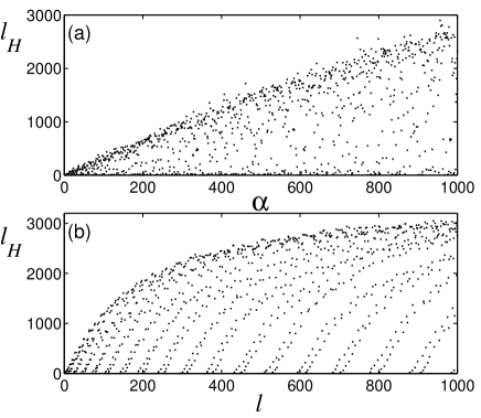
FIG. 1.: Localization measure $l_{H}$ for a rough surface with $N_{T}=100$ for $\epsilon=0.06$ and $d=b$; (a) for exact eigenstates $|~{}\alpha>$, (b) for individual LDOS $|~{}l>$.

In Fig. 1(a) the value of $l_{H}$ is plotted versus the index $\alpha$ for exact eigenstates ordered in energy $E^{\alpha}$. This typical dependence of $l_{H}$ on $\alpha$ is quite instructive. As one can anticipate, the number of principal components in the eigenstates increases, in average, with energy. On the other hand, for any large energy $E^{\alpha}$ there are many eigenstates that have small values of $l_{H}$. For understanding the origin of these strongly localized eigenstates (in the unperturbed basis $|~{}l>$), it is convenient to consider the so-called individual LDOS [8]. This quantity corresponds to the representation of an unperturbed state $|~{}l>$ in the basis of exact states $|\alpha>$. Using the definition (6) with ${\cal H}=\sum^{L}_{\alpha=1}w_{l}^{\alpha}\,\ln w_{l}^{\alpha}$ where the sum now runs over $\alpha$ for a specific value of $l$, one can characterize how many exact states contains specific unperturbed state $|~{}l>$.

The data of Fig. 1(b) show that there is a large number of unperturbed states that seem to be close to the exact ones (with $l_{H}\approx 1$). The important point is that these states appear in a regular way as a function of $l$. The analysis shows that exact eigenstates $|~{}\alpha>$ with smallest values of $l_{H}$ are originated from the unperturbed states with $m=1$, see Eq.(5). The data of Fig. 1(a) manifest that localized eigenstates $|~{}\alpha>$ with small values of $l_{H}$ can be classified by groups that are characterized by the values of $m=1,2,3\dots$ (for small $m$) of those unperturbed states $|~{}l>$ to which they are ”close”.

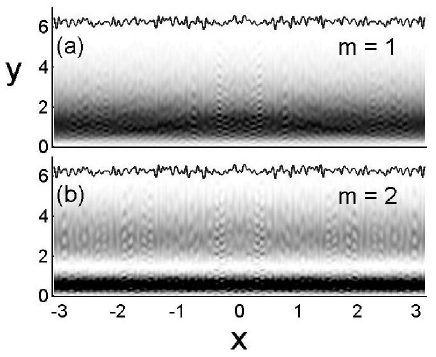
FIG. 2.: Examples of exact eigenstates that are strongly localized in energy representation; (a) $\alpha=968$ ($m=1$), (b) $\alpha=976$ ($m=2$). The probability $|\psi^{\alpha}(x,y)|^{2}$ is plotted for the parameters of Fig. 1 (dark regions correspond to high probablity). Broken horizontal curves show upper surface profiles.

Two examples of such eigenstates are given in Fig. 2 in the coordinate representation $(x,y)$. It is quite unexpected that these eigenstates are very different from the unperturbed ones even though they are quite close in energy representation. Fig. 2(a) shows that the rough boundary “pushes” the probability $|\psi^{\alpha}(x,y)|^{2}$ away from it, differing from the unperturbed mode with $m=1$ whose maximum is at the center, $y=d/2$. Similar repulsion occurs for $m=2$, see Fig. 2(b). Below we give the explanation of this phenomenon by making use of the Hamiltonian in variables $(u,v)$.

We start with the fact that eigenstates of the type shown in Fig. 2(a) are exponentially localized in the $m-$space (channel space) independently on $n$. Therefore, one can write, $C_{l}^{\alpha}(k)=C_{mn}^{\alpha}(k)\sim\exp\{-\beta(m-1)\}$ where $\beta$ is some constant (of the order of unity) determined by numerical data, and surprisingly independent of energy. Therefore, these localized eigenstates in the $(u,v)$ variables have the following form,

$$\psi_{loc}^{\alpha}=\frac{C}{g^{1/4}}e^{i(\chi+2\pi n_{\alpha}/b)u}\sum_{m=1}^{\infty}e^{-\beta(m-1)}\sin\left(\frac{m\pi v}{d}\right).$$ (7)

Here $C$ is the normalization constant determined by the orthonormality condition in curvilinear coordinates, $\int_{0}^{2\pi}\int_{0}^{1}dudv\sqrt{g}\psi_{loc}^{\alpha\ *}\psi_{loc}^{\alpha}=1$ (see [6] for details). As a result, one obtains,

$$\mid\psi_{loc}^{\alpha}(y)\mid^{2}=\frac{e^{2\beta}-1}{4\pi}\frac{\sin^{2}(\pi y/d)}{\cosh\beta-\cos(\pi y/d)}$$ (8)

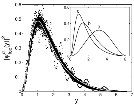
FIG. 3.: Projection of the eigenfuction profile of Fig. 2(a) onto the $y-$coordinate (dots), together with the analytical expression (8) (white curve). The value $\beta=0.53$ was numerically found by fitting $C_{mn}^{\alpha}(k)$ to the exponential dependence $\exp\{-\beta(m-1)\}$. In the inset, profiles (8) for strongly localized eigenstates with $m=1$ in dependence on the number $N_{T}$ of harmonics are shown for (a) $N_{T}=1$, $\beta\rightarrow\infty$, (b) $N_{T}=50$, $\beta=0.77$, and (c) $N_{T}\rightarrow\infty$, $\beta\rightarrow 0.48$.

The comparison of this expression with the numerical data is shown in Fig. 3. One can see that in spite of a relatively weak coupling of low channels ($m\sim 1$) to all others, the scattering from a rough surface strongly modifies the unperturbed states in $y-$direction. One can speak about a kind of “repulsion” of such eigenstates from the rough surface. In order to see how this repulsion depends on the degree of roughness, we have studied the form of the states with $m=1$ in dependence on the number $N_{T}$ of harmonics in the surface profile. The results shown in the inset, reveal that with an increase of $N_{T}$ the position of the maximum of the probability shifts away from the rough surface, and reaches its maximal value for $N_{T}\rightarrow\infty$ (practically, for $N_{T}=100$).

The eigenstates with small values of $l_{H}$ emerge in the energy spectrum for any energy, thus resulting in a very slow convergence to the limit of ergodicity. For example, the number of eigenstates originated from $m=1$ is $N_{m=1}(E)=\frac{2\pi}{d}\sqrt{E}$, therefore, the fraction of such eigenstates is given by $\frac{N_{m=1}(E)}{N(E)}=\frac{2b}{\pi^{2}}\frac{1}{\sqrt{E}}=\sqrt{\frac{4b}{\pi d}\frac{1}{N(E)}}$ where $N(E)$ is the total number of states with energy less than $E$. One should stress that in the energy spectrum these states appear regularily, due to the expression Eq.(5) with $m=1$ and different $n$.

FIG. 4.: Two eigenstates that are strongly localized in $x-$direction; (a) $\alpha=390$, (b) $\alpha=407$. The model parameters are the same as in Fig. 1.

We would like to note that the type of localization in the channel space we discuss here, is different from that studied for circular billiards with a rough surface (see, for example, [14]). The point is that in our case classical diffusion in the transverse momentum space turns out to be very strong compared with quantum localazation effects [15]. In contrast to circular billiards, in our model with quasi-1D geometry the effects of a strong localization (in the channel space) are due to the existence of a continuous set of classical horisontal trajectories (”bouncing balls”) which do not touch the rough boundary. As is shown in Ref. [16], these trajectories result in anomalous properties of conductance fluctuations for open waveguides of finite length.

It should be stressed that for any high energy one can find eigenstates of a very different structure. To demonstrate this fact, in Fig. 4 we report two typical examples of strongly localized (in the coordinate $x$) eigenstates. These eigenstates are widely spanned in the unperturbed basis of $\hat{H}^{0}$, with large values $l_{H}\gg 1$, and they correspond to large values of $m\ll 1$.

To conclude with, we have analysed the structure of eigenstates of a quasi-1D waveguide with a rough surface, paying main attentsion to their localization properties in the channel and coordinate representaion. Different sets of strongly delocalized eigenstates (along the waveguide) have been found, that have a quite specific form in the transverse direction. We have develop the approcah that allows one to explain this form, using the transformation to new canonical variables.

Another result is that eigenstates turn out to have very different localization properties and this difference can not be treated as a result of fluctuations only. Apart from the fluctuations, there are regular effects which are due to a strong influence of the geometry. Namely, it was found that the eigenstates originated from small values of $m$ are strongly localized (delocalized) in the channel (coordinate) representation, and those associated with large $m$ are strongly delocalized (localized) ones. This effect seems to be directly related to that found in Refs. [5, 17] for open finite waveguides, where it was shown that characteristic scales for scattering are different for different channels. Thus, it seems questionable whether standard statistical approaches based on completely random mathematical models, can adequately describe properties of eigenstates.

This work was supported by the CONACyT (Mexico) Grant No. 34668-E.

REFERENCES

- [1] Y.V. Fyodorov and A.D. Mirlin, Int. J. Mod. Phys. B, 8, 3795 (1994); K.B. Efetov, Supersymmetry in Disorder and Chaos (Cambridge University Press, Cambridge, England, 1997); A.D. Mirlin, Phys. Rep. 326, 259 (2000).
- [2] P. Sheng, Introduction to Wave Scattering, Localization, and Mesoscopic Phenomena (Academic Press, London, England, 1995).
- [3] I.V. Gornyi and A.D. Mirlin, Journ. Low Temp. Phys., 126, 1339 (2002).
- [4] A. García-Martín, J.A. Torres, J.J. Sáenz, and M. Nieto-Vesperinas, Appl. Phys. Lett. 71, 1912 (1997); A. García-Martín, J.J. Sáenz, and M. Nieto-Vesperinas, Phys. Rev. Lett. 84, 3578 (2000).
- [5] J.A. Sánchez-Gil, V. Freilikher, I. Yurkevich, and A.A. Maradudin, Phys. Rev. B 59, 5915 (1999).
- [6] G.A. Luna-Acosta, K. Na, L.E. Reichl, and A. Krokhin, Phys. Rev. E 53, 3271 (1996).
- [7] F.M. Izrailev, Physica Scripta, T90, 95 (2001).
- [8] G.A. Luna-Acosta, J.A. Méndez-Bermúrdez, and F.M. Izrailev, Phys. Lett. A 274, 192 (2000).
- [9] G.A. Luna-Acosta, A.A. Krokhin, M.A. Rodriguez, and P.H. Hernandez-Tejeda, Phys. Rev. B 54, 11410 (1996).
- [10] G.A. Luna-Acosta, M.A. Rodriguez, A.A. Krokhin, K. Na, and R.A. Méndez, Rev. Mex. Fis. 44, S3 7 (1998).
- [11] G.A. Luna-Acosta, J.A. Méndez-Bermúrdez, and F.M. Izrailev, Physica E 12, 267 (2002); Phys. Rev. E 65, 046605 (2002).
- [12] G.B. Akguc and L.E. Reichl, J. Stat. Phys. 98, 813 (2000); B. Huckestein, R. Ketzmerick, and C.H. Lewenkopf, Phys. Rev. Lett. 84, 5504 (2000); W. Li, L.E. Reichl, and B. Wu, Phys. Rev. E 65, 056220 (2002).
- [13] F.M. Izrailev, Phys. Rep. 196, 299 (1990).
- [14] F. Borgonovi, G. Casati, and B. Li, Phys. Rev. Lett. 77, 4744 (1996); K. Frahm and D.L. Shepelyansky, Phys. Rev. Lett. 78, 1440 (1997); Y. Hlushchuk et al, Phys. Rev. E 63, 046208 (2001).
- [15] J.A. Méndez-Bermúrdez, G.A. Luna-Acosta, and F.M. Izrailev, to be published.
- [16] M. Leadbeater, V.I. Falko, and C.J. Lambert, Phys. Rev. Lett. 81, 1274 (1998).
- [17] F.M. Izrailev and N.M. Makarov, Phys. Rev. B 67, 113402 (2003).