Specific heat of quasi-2D antiferromagnetic Heisenberg models with varying inter-planar couplings

Abstract

We have used the stochastic series expansion (SSE) quantum Monte Carlo (QMC) method to study the three-dimensional (3D) antiferromagnetic Heisenberg model on cubic lattices with in-plane coupling $J$ and varying inter-plane coupling $J_{\perp}<J$. The specific heat curves exhibit a 3D ordering peak as well as a broad maximum arising from short-range 2D order. For $J_{\perp}\ll J$, there is a clear separation of the two peaks. In the simulations, the contributions to the total specific heat from the ordering across and within the layers can be separated, and this enables us to study in detail the 3D peak around $T_{c}$ (which otherwise typically is dominated by statistical noise). We find that the peak height decreases with decreasing $J_{\perp}$, becoming nearly linear below $J_{\perp}=0.2J$. The relevance of these results to the lack of observed specific heat anomaly at the ordering transition of some quasi-2D antiferromagnets is discussed.

I Introduction

Spatially anisotropic systems and dimensional crossovers have been issues of theoretical and experimental interest for many decades, especially in context of classical critical phenomena.stanley1 ; stanley2 In recent years, a large number of quasi-low dimensional, low-spin, spatially anisotropic materials have been synthesized and their properties investigated in great detail. This has led to a renewed interest in these issues including the role of enhanced quantum fluctuations.sudip ; carlson ; bocquet ; affleck Perhaps the most studied of these are the cuprate family of materials, whose parent stoichiometric compounds are antiferromagnetic insulators which upon doping become high temperature superconductors. These are layered compounds, where exchange coupling between the planes is many orders of magnitude smaller than the exchange coupling in the planes.CHN ; chubukov However, these are by no means the only systems where spatial anisotropy and dimensional crossovers are important. The list of just novel transition-metal oxide materials, which despite their low-dimensionality often develop 3-dimensional long-range order, includes several cuprates, vanadates, copper-germenates, pnictide oxides, manganites, etc.review

In these materials both spatial anisotropy and anisotropy in spin-space can be important in the development of 3D order. For example, it is quite possible that in some cuprate families XY anisotropy plays an important role in bringing about long-range order, while in others it is the interplanar coupling which is primarily responsible for the transition. Here, we will focus on layered systems with SU(2) symmetry in spin-space. This is believed to be relevant to the material La₂CuO₄. At the finite temperature 3D transition, one expects the universality class for such a system to be that of classical 3D Heisenberg model. However, in La₂CuO₄ no specific heat anomaly is seen at the 3D transition,sun contrary to expectations for the 3D classical Heisenberg model. In this paper we use a quantum Monte Carlo (QMC) method to verify that the transition in spatially anisotropic systems remains in the universality class of 3D classical Heisenberg model. Our primary goal is to clarify how the amplitude for the specific-heat anomaly at the transition is diminished in systems with weak interplanar couplings. This would help us predict which of the newly synthesized systems should show such anomalies, given the finite experimental resolution.

A simple way to understand the reduction in the amplitude for the specific heat anomaly, in these systems, is to consider the effect of preexisting short-range order at the transition. In a spatially anisotropic system, short range order in the planes can develop at temperatures much above the 3D ordering temperature. And, if the system is highly anisotropic, substantial spin-correlations can develop in the planes before the eventual 3D transition. This means the effective number of degrees of freedom involved in the 3D order is substantially reduced. Hence, the specific-heat anomaly must diminish. Our goal is to obtain a quantitative estimate for this effect.

The rest of the paper is organized as follows. We introduce the model and the computational techniques used in Sec. II. The results of the simulations and the related discussions are presented in Secs. III and IV. We conclude in Sec. V with a summary of the results.

II Models and Simulation technique

We have studied the Heisenberg antiferromagnet on an anisotropic cubic lattice. This model is given by the Hamiltonian

$$H=J\sum_{\langle i,j\rangle_{xy}}{\bf S}_{i}\cdot{\bf S}_{j}+J_{\perp}\sum_{\langle i,j\rangle_{z}}{\bf S}_{i}\cdot{\bf S}_{j}$$ (1)

where $J$ ($J_{\perp}$) is the strength of the intra- (inter-) planar coupling. The first (second) summation refers to summing over all nearest neighbors parallel (perpendicular) to the XY-plane. We will study the model as a function of the dimensionless inter-plane coupling $\alpha=J_{\perp}/J$.

Figure 1: Spin stiffness vs. temperature for different systems with the same aspect ratio. The upper (lower) panel shows the stiffness perpendicular (parallel) to the planes.

The stochastic series expansion (SSE) method sse1 ; sse2 is a finite-temperature QMC technique based on importance sampling of the diagonal matrix elements of the density matrix $e^{-\beta H}$. There are no approximations beyond statistical errors. Using the “operator-loop” cluster update,sse2 the autocorrelation time for the system sizes we consider here (up to $\approx 3\times 10^{4}$ spins) is at most a few Monte Carlo sweeps even at the critical temperature.dloops

On the dense temperature grids that we need in order to study the critical region in detail, we have further found that the statistics of the data obtained can be significantly improved by the use of a tempering scheme. tempering1 ; tempering2 A standard single-process tempering method, where the temperature of the simulation fluctuates on a grid of pre-selected temperatures, was previously used in a study of the isotropic 3D Heisenberg model.aws1 Here we use parallel tempering, tempering2 where several simulations are run simultaneously on a parallel computer, using a fixed value of $\alpha$ and different, but closely spaced, values of $T$ at and around the critical temperature. Along with the usual Monte Carlo updates, we attempt to swap the temperatures of SSE configurations (processes) with adjacent values of $T$ at regular intervals (typically after every Monte Carlo step, each time attempting several hundred swaps) according to a scheme that maintains detailed balance in the space of the parallel simulations. This has favorable effects on the simulation dynamics, as the temperature of the SSE configurations will fluctuate across the critical temperature. More importantly in the case considered here, a given configuration will contribute to measured expectation values at several nearby temperatures, thereby reducing the over-all statistical errors (at the cost of introducing correlations between the errors, which is of minor significance here). Implementation of tempering schemes in the context of the SSE method have been discussed in Ref. bow, .

The thermodynamics of the 3D Heisenberg model on an isotropic simple cubic lattice are fairly well understood from both analytic and computational studies.baker ; oitmaa ; sauerwein Recent large scale Monte Carlo studiesaws1 ; dloops have resulted in an accurate estimate of the critical temperature, $T_{c}/J\approx 0.946$. Several approximations also exist for $T_{c}$ of the anisotropic model.oguchi ; liu ; CHN ; katanin For weak coupling between the planes, the interplanar couplings can be treated in mean-field theory and lead to the relation $T_{c}\sim-1/\mbox{ln}(\alpha)$.CHN We are not aware of any previous calculations of the specific heat of anisotropic systems.

III Locating the transition temperature

We first determine the transition temperature for the model as a function of $\alpha$. An efficient way to do this is by studying the scaling properties of the spin-stiffness. We have evaluated the spin stiffnesses both parallel to and perpendicular to the planes. The stiffness can be defined kohn ; kopietz as the second derivative of the free energy with respect to a uniform twist $\phi$:

$$\rho=\frac{\partial^{2}F(\phi)}{\partial\phi^{2}}.$$ (2)

The stiffness can also be related to the fluctuations of the “winding number” in the simulations pollock ; harada ; sse1 ; cuccoli and hence can be estimated directly without actually including a twist. Since the twist can be applied parallel to or perpendicular to the planes, there are two different spin stiffnesses, $\rho_{x}$ and $\rho_{z}$, in the anisotropic system considered here.

For a system of weakly coupled Heisenberg chains, it has been shown that estimates for various observables for a spatially anisotropic system can depend non-monotonically on the system size for square lattices. multichain One can instead use rectangular lattices to more rapidly obtain monotonic behavior of the numerical results for extrapolating to the thermodynamic limit. We expect similar effects in the present model at $\alpha\ll 1$. Hence we have studied tetragonal lattices with $L_{x}=L_{y}\neq L_{z}$. Lattices with an aspect ratio $R=L_{x}/L_{z}=4$ have been used to obtain the results presented here. We have chosen six different values of $\alpha$, of the form of $\alpha=2^{-n},n=1,\ldots,6$.

Following Ref. aws1, , we use the finite-size and temperature dependence of the spin stiffnesses to determine the critical temperature. barber For a fixed aspect ratio, the stiffness at $T_{\rm c}$ is predicted to scale as

$$\rho_{\mu}=L_{\mu}^{2-d},~{}~{}~{}\mu=x,z$$ (3)

where $d$ is the dimensionality of the system. The above relation implies that for the 3D Heisenberg model, on a plot of $L_{\mu}\rho_{\mu}$ as a function of $T$ the curves for different system sizes will cross each other at $T_{c}$. Results for $\alpha=1/4$ are shown in Fig. 1. The upper (lower) panel shows $L_{x}\rho_{x}$ ($L_{z}\rho_{z}$) versus $T$ for four different system sizes. The curves indeed intersect each other almost at a single point. Subleading corrections are seen in the fact that the crossing points move slightly as the system size is increased. Interestingly, the behavior is opposite for the two stiffness constants; in the case of $\rho_{x}$ the crossings move down in temperatures, whereas the $\rho_{z}$ crossings move up. Hence, we believe that the crossings for the two largest system sizes bracket the true $T_{c}$ and we view them as the upper and lower bounds. From these results we estimate $T_{c}=0.6160\pm 0.0005$ for $\alpha=1/4$.

Figure 2: Finite-size scaling of the staggered susceptibility at $\alpha=1/4$. (a) Size dependence close to $T_{c}$. At $T_{c}$, the data are expected to fall on a straight line with slope $-\eta=-0.037$, which is indicated with the dotted line. (b) Scaling plot above $T_{c}$, using $T_{c}/J=0.616$ and the 3D classical Heisenberg exponents $\eta=0.037$ and $\nu=0.711$.

Next we study the universality class of the transition. To this end, we consider the static magnetic susceptibility, defined as

$$\chi({\bf q})={1\over N}\sum_{\langle i,j\rangle}e^{i{\bf q}\cdot({\bf r}_{j}-{\bf r}_{j})}\int^{\beta}_{0}d\tau\langle S^{z}_{j}(\tau)S^{z}_{i}(0)\rangle,$$ (4)

where $N=L_{x}^{2}L_{y}$ is the size of the system. At the critical temperature, the staggered susceptibility $\chi({\bf Q})$ should scale barber with the system length as $L_{x}^{2-\eta}$, where ${\bf Q}=(\pi,\pi,\pi)$ is the 3D ordering wave vector. For any non-zero value of $J_{\perp}$, the transition is expected to belong to the classical 3D Heisenberg universality class, for which the critical exponents are known to a high degree of accuracy. campostrini The spin-spin correlation function exponent $\eta\approx 0.037$. Figure 2(a) shows $\alpha=1/4$ results for ${\mbox{ln}}(\chi({\bf Q})/L_{x}^{2})$ versus ln($L_{x}$) at temperatures close to $T_{c}$. Asymptotically, we expect the data to fall on a straight line with slope $-\eta\approx-0.037$ at $T=T_{c}$ and diverge upward (downward) for $T<T_{c}$ ($T>T_{c}$). This is indeed what we observe. The curves are completely consistent with the known value of $\eta$ and the estimate of $T_{c}$ obtained from Fig. 1.

We have also tested the expected scaling for $T>T_{c}$. In the thermodynamic limit, $\chi({\bf Q})$ should diverge as $t^{-\gamma}$, where $t=|T-T_{c}|$ and $\gamma=\nu(2-\eta)$. For a finite system, finite-size scaling predicts $\chi_{L}(t)=\chi_{\infty}(t)f[\xi(t)/L]$, with the correlation length diverging as $\xi\sim t^{-\nu}$. Hence on a plot of $\chi_{L}(t)t^{\gamma}$ versus $Lt^{\nu}$, data for different $L$ should collapse onto a single curve. As shown in Fig. 2(b), this is indeed the case with our estimated $T_{c}$ and the known 3D Heisenberg exponents.

We have here discussed the determination of $T_{c}$ and checked the consistency with the expected universality class for $\alpha=1/4$. Using the spin stiffness scaling, we have located $T_{c}$ for several couplings $\alpha$. The results are graphed in Fig. 3. We compare our results with the expression obtained by Liu,liu

$${1\over T_{c}}={1\over\pi^{3}}\int_{0}^{\pi}\int_{0}^{\pi}\int_{0}^{\pi}{\frac{dk_{x}dk_{y}dk_{z}}{2-\mbox{cos}k_{x}\mbox{cos}k_{y}+\alpha(1-\mbox{cos}k_{z})}}.$$ (5)

We find that while this equation gives a reasonable estimate for $T_{c}(\alpha)/T_{c}(1)$ for $\alpha$ close to unity, it begins to deviate substantially from the SSE results for small $\alpha$.

Figure 3: Ratio of the critical temperature for the anisotropic system to that for the isotropic system as a function of the anisotropy. The circles denote the results from Eq. 5.

IV Calculations of the specific heat

Having determined $T_{c}$ as a function of $\alpha$, we now present the results for the specific heat calculations. The specific heat is defined as the temperature derivative of the energy, $C_{v}=(\partial E/\partial T)/N$. As discussed in Appendix A, the SSE method allows us to obtain a direct estimate of the specific heat from the operator sequence in the simulation, so that any additional noise in the data due to numerical differentiation of the energy function can be avoided (although the two approaches in practice give very similar results). The SSE estimator for the total specific heat (i.e., not normalized by the lattice size) is

$$NC_{v}=\langle n^{2}\rangle-\langle n\rangle^{2}-\langle n\rangle,$$ (6)

where $n$ is the power-series expansion order (the number of bond operators in the SSE operator string), which fluctuates in the simulations. We will be interested in the contributions to $C_{v}$ from the spin-spin ordering across and within the layers close to $T_{c}$. Decomposing the Hamiltonian into an in-plane term $H_{p}$ and an inter-layer term $H_{z}$, the specific heat

$$C_{v}=(\partial\langle H_{\rm p}\rangle/\partial T+\partial\langle H_{z}\rangle/\partial T)/N=C_{v}^{p}+C_{v}^{z}.$$ (7)

The SSE estimators for the two terms are given in terms of the numbers of bond operators in the expansion acting within a single layer ($n_{p}$) and between two layers ($n_{z}$):

$$NC^{p}_{v} = \langle n_{p}^{2}\rangle+\langle n_{p}n_{z}\rangle-\langle n_{p}\rangle^{2}-\langle n_{p}\rangle\langle n_{z}\rangle-\langle n_{p}\rangle,$$ (8)

$$NC^{z}_{v} = \langle n_{z}^{2}\rangle+\langle n_{p}n_{z}\rangle-\langle n_{z}\rangle^{2}-\langle n_{p}\rangle\langle n_{z}\rangle-\langle n_{z}\rangle.$$ (9)

These expressions suggest the possibility of a different decomposition of the specific heat. We will define $C_{v}^{\rm plane}$ as the part of the estimator (8) that contains only purely in-plane contributions:

$$C^{\rm plane}_{v}=(\langle n_{p}^{2}\rangle-\langle n_{p}\rangle^{2}-\langle n_{p}\rangle)/N.$$ (10)

We refer to the remaining part of the total susceptibility as the 3D contribution, i.e.,

$$C^{\rm 3D}_{v}=C_{v}-C^{\rm plane}_{v}=C^{\rm inter}_{v}+C^{\rm cross}_{v},$$ (11)

where the purely inter-plane contribution $C^{\rm inter}_{v}$ and cross-term $C^{\rm cross}_{v}$ are given by

$$C^{\rm inter}_{v} = (\langle n_{z}^{2}\rangle-\langle n_{z}\rangle^{2}-\langle n_{z}\rangle)/N,$$ (12)

$$C^{\rm cross}_{v} = 2(\langle n_{p}n_{z}\rangle-\langle n_{p}\rangle\langle n_{z}\rangle)/N,$$ (13)

We will show that the cross-term, half of which appears both in Eq. (8) and Eq. (9), dominates in the 3D contribution (11). The advantage of considering separately the different contributions to $C_{v}$, either in the form of (7) or (11) and, is that the full specific heat is dominated by the in-plane term and the other contributions can be difficult to discern due to statistical fluctuations. We will here focus in particular on the 3D contribution (11).

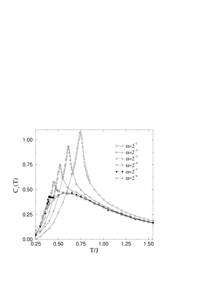
Figure 4: The specific heat over a wide range of temperature for several different anisotropies. The system size is $48\times 48\times 12$. The separation of the 3D ordering peak from the broad maximum arising out of the 2D physics is clearly visible for $\alpha\leq 2^{-3}$.

The specific heat for the 3D Heisenberg model on highly anisotropic lattices ($\alpha\ll 1$) will have two separate peaks, reflecting the 2D physics and the 3D ordering. The Mermin-Wagner theorem dictates that there can be no long-range order at $T>0$ in a strictly 2D system with a continuous symmetry. The correlation length then diverges exponentially CHN as $T\to 0$, and the specific heat has a broad maximum at $T/J\approx 0.7$.c2dcalc This broad maximum is the dominant feature of the specific heat curve also for small inter-planar couplings. On the other hand, for any $\alpha>0$ there is a phase transition to an ordered state at $T_{c}>0$, as we have discussed in Sec. III. The signature of this phase transition in the specific heat should be a peak at $T_{c}$. Since the transition belongs to the 3D Heisenberg universality class, there should a cusp-like singularity (instead of a divergent singularity) and the peak height is finite.

SSE results for the specific heat over a wide temperature range are shown in Fig. 4 for a system of size $N=48\times 48\times 12$. The effects of finite system size on the position of the peak and the peak height will be discussed later. The separation of the 3D ordering peak from the broad maximum arising out of the 2D physics is clearly seen for $\alpha\leq 2^{-3}$. It is also seen that the excess peak height over the 2D background decreases rapidly with decreasing $\alpha$, becoming hard to discern for $\alpha<2^{-5}$.

Figure 5: The 3D contribution to the specific heat for several different anisotropies, $\alpha$, and for three different system sizes. Results for the purely inter-plane term $C_{v}^{\rm inter}$ are also shown for the three largest couplings (for the largest system size only).

Since the specific heat curve is dominated by its 2D contribution when $\alpha\ll 1$, it is extremely difficult to study the nature of the 3D peak near $T_{c}$. However, the 3D contribution (11) can be studied to a high degree of accuracy. Results for several couplings $\alpha$ and system sizes are shown in Fig. 5. Several features are immediately apparent. The 3D contribution peaks at the Néel temperature and rapidly decreases away from it. The peak position moves only slightly with increasing system size. The estimates of $T_{c}$ obtained from the position of the peaks are in close agreement with the more accurate estimates we obtained in Sec. III using the spin stiffness. In Fig. 5 we also show some results for the purely inter-plane contribution $C_{v}^{\rm inter}$ to $C_{v}^{\rm 3D}$, which is seen to be small and decreasing relative to the full 3D contribution as $\alpha\to 0$. This is expected, as the estimator (12) implicitly contains a prefactor proportional to $\alpha^{2}$, whereas the cross-term (13) contains a linear $\alpha$ dependence.

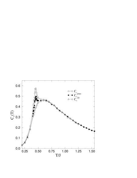
Figure 6: The specific heat and its in-plane contribution for $\alpha=2^{-4}$. The anomalies at the transition temperature is clearly visible for both. The system size is $48\times 48\times 12$. For comparison, the specific heat for the pure 2D Heisenberg model is also shown.

Figure 7: The excess in $C_{v}^{\mbox{\tiny{plane}}}(T_{c})$ over the specific heat of the pure 2D Heisenberg model at the 3D $T_{c}$, normalized by the corresponding 3D contribution to the total specific heat. The system size is $48\times 48\times 12$.

While the specific heat anomaly is most pronounced in the 3D contribution, it is also present in the purely in-plane term. This is shown in Fig. 6, where we have graphed the total specific heat and the purely in-plane contribution at $\alpha=1/16$, where the 3D ordering peak is well separated from the broad 2D maximum. We compare these results with the specific heat $C_{v}^{\mbox{\tiny{2D}}}$ for a 2D system ($\alpha=0$). As expected, the in-plane term for the 3D system is dominated by a broad maximum and coincides closely with the specific heat of the 2D system away from $T_{c}$. However, there is also a distinct peak at the 3D transition temperature. In order to quantify the relative sizes of the ordering peaks in $C_{v}^{\rm 3D}$ and $C_{v}^{\rm plane}$, we next consider the excess at $T_{c}$ of the in-plane contribution over the specific heat of the pure 2D system model at the same temperature. Its ratio to the 3D contribution is graphed as a function of the coupling $\alpha$ in Fig. 7. As $\alpha\to 0$, this ratio appears to converge to a value $\approx 1$, or, in other word, the ordering peak in the in-plane contribution becomes nearly equal to that of the 3D contribution.

The peak height $C_{v}^{\mbox{\tiny{3D}}}(T_{c})$ decreases rapidly with decreasing $\alpha$. To get a more quantitative estimate of the nature of its variation with $\alpha$, we have extracted the thermodynamic peak height for different $\alpha$. The specific heat exponent, which governs the scaling of the peak to infinite size, is small (and negative), campostrini and the statistical errors of our data are relatively large for small $\alpha$. The extrapolation is therefore affected by some uncertainty that is not easy to quantify precisely. Our results are shown in Fig. 8. For small $\alpha$, the peak height is nearly linear in $\alpha$. This behavior can be roughly understood by the argument that the specific heat anomaly should scale as $1/\xi^{2}$, where $\xi$ is the correlation length of the $2D$ system at the 3D transition temperature. Furthermore, the 3D correlations become significant and lead to the 3D transition CHN when $\xi^{2}\alpha\approx 1$. Thus the amplitude for the specific heat anomaly should vanish linearly with $\alpha$. It would be interesting to compare the specific heat anomaly of various quasi-2D Heisenberg systems against this result.

V Conclusions

In this paper we have studied the 3D ordering transition in a model of weakly coupled Heisenberg planes. Our results on the transition temperature and universality class of the transition are in accord with general expectations. Our primary focus here was on the specific heat and in particular on the specific heat anomaly at the 3D ordering transition. We find that for small $J_{\perp}$ the amplitude for the specific heat anomaly is a nearly linear function of $J_{\perp}$. It should be possible to compare this result directly against experiments on various anisotropic materials. However, it is clear that for highly anisotropic systems (such as La₂CuO₄, where the anisotropy maybe as small as $10^{-6}$) such anomalies will be very difficult to detect above the background.

Figure 8: The peak height for the 3D ordering extrapolated to the thermodynamic limit as a function of the anisotropy. For small anisotropies, the peak height increases approximately linearly with the anisotropy.

Appendix A The SSE method

The SSE method has been discussed in several papers.sse1 ; sse2 ; dloops Here we present a brief outline of the method in order to discuss the estimator for the specific heat. For the present case, the SSE approach starts by casting the Hamiltonian in the form

$${\hat{H}}=-{1\over 2}\sum_{b=1}^{3N}[{\hat{H}}_{1,b}-{\hat{H}}_{2,b}]+C,$$ (14)

where $b$ denotes the bond connecting the nearest neighbor sites $\langle i(b),j(b)\rangle$, $C$ is an additive constant and the operators $H_{1,b}$ and $H_{2,b}$ are defined as

$$H_{1,b} = 2J(b)[{1\over 4}-S_{i(b)}^{z}S_{j(b)}^{z}],$$ (15)

$$H_{2,b} = J(b)[S_{i(b)}^{+}S_{j(b)}^{-}+S_{i(b)}^{-}S_{j(b)}^{+}].$$ (16)

The coupling constant $J(b)=J$ for bonds in the planes and $J(b)=J_{\perp}$ for inter-planar bonds. An exact and useful expression for an operator expectation value at inverse temperature $\beta=J/T$,

$$\langle{\hat{A}}\rangle={1\over Z}{\mbox{Tr}}\{{\hat{A}}e^{-\beta{\hat{H}}}\},\hskip 14.45377ptZ={\mbox{Tr}}\{e^{-\beta{\hat{H}}}\},$$ (17)

is obtained by expanding the density matrix $e^{-\beta{\hat{H}}}$ in a Taylor series and writing the trace as sum over the diagonal matrix elements in a basis $\{|\alpha\rangle\}=\{|S_{1}^{z},\ldots,S_{N}^{z}\rangle\}$. The partition function can then be written as

$$Z = \sum_{n=0}^{\infty}\sum_{\alpha}\sum_{S_{n}}{\frac{\beta^{n}}{n!}}\langle\alpha|\prod_{p=1}^{n}H_{a_{p},b_{p}}|\alpha\rangle,$$ (18)

$$\equiv \sum_{n=0}^{\infty}\beta^{n}\sum_{\alpha}\sum_{S_{n}}W^{\prime}(\alpha,S_{n})$$ (19)

where $S_{n}$ denotes a sequence of index pairs defining the operator string $\prod_{p=1}^{n}H_{a_{p},b_{p}}$:

$$S_{n}=[a_{1},b_{1}][a_{2},b_{2}]\dots[a_{n},b_{n}],$$ (20)

where $a\in\{1,2,3\}$, $b\in\{1,\dots,N\}$. We have separated the temperature dependence of the weight factor for convenience. We can now write the expectation value of an operator as

$$\langle{\hat{A}}\rangle_{W}={1\over Z}\sum_{n=0}^{\infty}\beta^{n}\sum_{\alpha}\sum_{S_{n}}A(\alpha,S_{n})W^{\prime}(\alpha,S_{n}).$$ (21)

Taking ${\hat{A}}={\hat{H}}$, it can be shownsse1 ; handscomb that the energy is given by the average length of the operator sequences

$$E=-{1\over\beta Z}\sum_{n=0}^{\infty}n\beta^{n}\sum_{\alpha}\sum_{S_{n}}W^{\prime}(\alpha,S_{n})\equiv-{1\over\beta}\langle n\rangle.$$ (22)

A straightforward differentiation with respect to temperature gives the specific heat $C_{v}=\frac{\partial E}{\partial T}$ in the form of Eq. (6).

References

- (1) L. L. Liu, and H. E. Stanley, Phys Rev. Lett 29, 927 (1972).
- (2) L. J. de Jongh, and H. E. Stanley, Phys. Rev. Lett. 36, 817 (1976).
- (3) S. Chakravarty, Phys. Rev. Lett. 77, 4446 (1996).
- (4) E. W. Carlson, D. Orgad, S. A. Kivelson, and V. J. Emery, Phys. Rev. B 62, 3422 (2000).
- (5) M. Bocquet, F. H. L. Essler, A. M. Tsvelik, and A. O. Gogolin, Phys. Rev. B 64, 94425 (2001).
- (6) I. Affleck, M. P. Gelfand, and R. R. P. Singh, J. Phys. A 27(22), 7313 (1994); I. Affleck, and B. I. Halperin, ibid.29(11), 2627 (1996).
- (7) S. Chakravarty, B. I. Halperin, and D. R. Nelson, Phys. Rev. Lett. 60, 1057 (1988); Phys. Rev. B 39, 2344 (1989).
- (8) A. V. Chubukov, S. Sachdev, and J. Ye, Phys. Rev. B 49, 11919 (1994).
- (9) R. R. P. Singh, W. E. Pickett, D. W. Hone, and D. J. Scalapino, Comments on Modern Physics 2(1), B1 (2000).
- (10) K. Sun, J. H. Cho, F. C. Chou, W. C. Lee, L. L. Miller, D. C. Johnston, Y. Hidaka, and T. Murakami, Phys. Rev. B 43, 239 (1991).
- (11) G. S. Rushbrooke, G. A. Baker, and P. J. Wood, in Phase Transitions and Critical Phenomena, ed. C. Domb and M. S. Green, Academic Press, 1981.
- (12) J. Oitmaa, C. J. Hamer, and Z. Weihong, Phys. Rev. B 50, 3877 (1994).
- (13) R. A. Sauerwein and M. J. De Oliveira, Mod. Phys. Lett. B 9, 619 (1995).
- (14) A. W. Sandvik, Phys. Rev. Lett. 80, 5196 (1998).
- (15) T. Oguchi, Phys. Rev. 133, A1098 (1964).
- (16) S. H. Liu, J. Magn. Magn. Mater. 82, 294 (1989).
- (17) V. Yu. Irkhin and A. A. Katanin, Phys. Rev. B 55, 12 318 (1997); ibid.57, 379 (1998).
- (18) I. G. Araújo, J. R. de Sousa, and N. S. Branco, Physica A 305, 585 (2002).
- (19) A. W. Sandvik and J. Kurkijärvi, Phys. Rev. B 43, 5950 (1991); A. W. Sandvik, Phys. Rev. B 56, 11678 (1997).
- (20) A. W. Sandvik, Phys. Rev. B 59, R14157 (1999).
- (21) O. F. Syljuåsen and A. W. Sandvik, Phys. Rev. E 66, 046701 (2002).
- (22) E. Marinari, Lecture Notes in Physics, Vol. 501 Advances in computer simulation: lectures held at the Eötvös Summer School in Budapest, Hungary, 16-20, July 1996, edited by J. Kertsz and I. Kondor (Springer, 1998).
- (23) K. Hukushima, H. Takayama, K. Nemoto, Int. J. Mod. Phys. C 7, 337 (1996); K. Hukushima, K. Nemoto, J. Phys. Soc. Jpn. 65, 1604 (1996)
- (24) P. Sengupta, A. W. Sandvik, and D. K. Campbell, Phys. Rev. B 65, 155113 (2002).
- (25) W. Kohn, Phys. Rev. 133, A171 (1964).
- (26) P. Kopietz, Phys. Rev. B 57, 7829 (1998).
- (27) E. L. Pollock and D. M. Ceperley, Phys. Rev. B 36, 8343 (1987).
- (28) K. Harada and N. Kawashima Phys. Rev. B 55, R11949 (1998).
- (29) A. Cuccoli, T. Roscilde, V. Tognetti, R. Vaia, and P. Verrucchi, cond-mat/0209316.
- (30) A. W. Sandvik, Phys. Rev. Lett. 83, 3069 (1999).
- (31) For a review of finite-size scaling, see: M. N. Barber in Phase Transitions and Critical Phenomena, Vol. 8, ed. Domb and Lebowitz (Academic Press, 1983).
- (32) M. Campostrini, M. Hasenbusch, A. Pelissetto, P. Rossi, and E. Vicari, Phys. Rev. B 65, 144520 (2002).
- (33) G. Gomez-Santos, J. D. Joannopoulos, and J. W. Negele, Phys. Rev. B 39, 4435 (1989); J.-K. Kim and M. Troyer, Phys. Rev. Lett. 80, 2705 (1998).
- (34) D. C. Handscomb, Proc. Cambridge Philos. Soc. 58, 594 (1962); 60, 115 (1964).