Amplitude and Gradient Scattering in Waveguides with Corrugated Surfaces

Abstract

We study chaotic properties of eigenstates for periodic quasi-1D waveguides with ”regular” and ”random” surfaces. Main attention is paid to the role of the so-called ”gradient scattering” which is due to large gradients in the scattering walls. We demonstrate numerically and explain theoretically that the gradient scattering can be quite strong even if the amplitude of scattering profiles is very small in comparison with the width of waveguides.

During last decade much attention has been paid to the theory of quasi-1D disordered solids with the so-called bulk scattering. By this term one describes the situation where the whole volume of a scattering region contains scatters whose density determines the mean free path $\lambda$ for a propagation of electrons. According to the theory, apart from $\lambda$, transport properties of finite samples are described by two other characteristic lengths: size $L$ of a sample and localization length  $l_{\infty}$. The latter is deterimied by the degree of the decrease of the amplitude of eigenstates along infinite samples with the same scattering characteristics. The core of the modern theory of the transport for such quasi-1D systems is the so-called single-parameter scaling. It was shown that when the mean free path is much less than both $L$ and $l_{\infty}$, all statistical characteristics of the transport are fully described by the only scaling parameter which is the ratio of the localization length to the size of a sample (see, e.g. [1] and references therein).

Another kind of quasi-1D systems that has attracted much attention in past few years, is the many-mode waveguide with rough surfaces. In this case the scattering is entirely related to statistical characteristics of scattering walls, therefore, one can speak about surface scattering. For some time it was believed that the surface scattering can be analytically described by modified methods thoroughly developed for bulk scattering. However, recent numerical studies of such systems [2, 3] have revealed a principal difference between surface and bulk scattering (see discussion and references in [4]). Specifically, it was found that the transport through quasi-1D waveguides with rough surfaces essentially depends on many characteristic lengths, not on one length as in the case of the bulk scattering. This fact is due to a non-isotropic character of scattering in the channel space. In particular, the transmission coefficient smoothly decreases with an increase of the angle of incoming waves, since characterictic lengths for backscattering are different for different channels [3, 5].

The latter subject of the surface scattering has a direct link to the problem of quantum chaos. The point is that the waveguides with rough walls can be treated from the viewpoint of classical and quantum mechanics that describe a particle moving inside billiards and having multiple reflections from the walls. One of the problems of quantum chaos is the quantum- classical correspondence for the situation when, in the classical limit, global properties of the motion of a particle are strongly chaotic. More specifically, it is of great interest to find what is the fingerprint of classical chaos in quantum eigenstates of closed/periodic billiards, as well as the relation of statistical properties of the transport through open billiards to the underlying classical chaos.

In this paper we investigate the properties of quantum eigenstates of billiards with regular and rough walls, with the application to the wave scattering through quasi-1D waveguides with surface scattering. To be specific, we consider quasi-1D waveguides that are periodic in the $x-$direction with period $2\pi$. The upper and low walls are given by the functions, $f_{1}(x)=f_{1}(x+2\pi)=d+a_{1}\xi_{1}(x)$ and $f_{2}(x)=f_{2}(x+2\pi)=a_{2}\xi_{2}(x)$ where $d$ is the average width of the waveguides and $a_{1,2}\ll d$ stands for the amplitude of the scattering walls. Our interest is in the structure of eigenstates of the corresponding Hamiltonian with zero boundary conditions on the two walls.

For our purpose it is convenient to pass to the variables $u=x,\ v=\frac{f_{2}(x)-y}{f_{2}(x)-f_{1}(x)}$ in which the new Hamiltonian $\hat{H}=\hat{H}^{0}+\hat{V}$ describes a particle moving inside a waveguide with flat boundaries in new $u,v$ coordinates (see details in [6]). Here $\hat{H}^{0}=\frac{1}{2m_{e}}(\hat{P}_{u}^{2}+\hat{P}_{v}^{2})$ and the effective potential $\hat{V}(u,v,\hat{P}_{u},\hat{P}_{v})$ depends on the functions $f_{1}$ and $f_{2}$, with $\hat{P}_{u},\hat{P}_{v}$ as the canonical momentums. The solution of the Schrödinger equation for $\hat{H}$ can be written in the form $\psi_{E}(u,v)=\exp(i\chi)\,\psi_{\chi}(u,v)$. Since statistical properties of eigenstates of $\hat{H}$ do not depend on specific value of the Bloch index $\chi$ inside the first Brillouin band, all numerical data were obtained for a specific value of $\chi$. By expanding $\psi_{\chi}(u,v)$ in the basis of $\hat{H}_{0}$, one can find the matrix representaion of $\hat{H}$ in the unperturbed basis specified by the two indexes $n$ and $m$ [7].

The Hamiltonian matrix elements are given by

$$H^{k}_{mnm^{\prime}n^{\prime}} = \frac{\hbar^{2}}{2\pi}\left\{\pi(n+k)^{2}\delta_{nn^{\prime}}\delta_{mm^{\prime}}+\left[\frac{m^{2}\pi^{2}}{2}\left(J^{2}_{n^{\prime}n}+J^{3}_{n^{\prime}n}+J^{6}_{n^{\prime}n}\right)+\left(\frac{1}{8}+\frac{m^{2}\pi^{2}}{6}\right)J^{4}_{n^{\prime}n}\right]\delta_{mm^{\prime}}\right.$$ (1)

$$+ i(n+n^{\prime}+2k)\frac{mm^{\prime}}{m^{2}-m^{\prime 2}}\left[J^{1}_{n^{\prime}n}-(-1)^{m+m^{\prime}}\left(J^{1}_{n^{\prime}n}+J^{5}_{n^{\prime}n}\right)\right]$$ (2)

$$+ \left.\frac{2mm^{\prime}(m^{2}+m^{\prime 2})}{(m^{2}-m^{\prime 2})^{2}}\left[-J^{6}_{n^{\prime}n}+(-1)^{m+m^{\prime}}\left(J^{6}_{n^{\prime}n}+J^{4}_{n^{\prime}n}\right)\right]\right\}$$ (3)

where

$$J^{1}_{n^{\prime}n}=\int^{2\pi}_{0}\frac{f_{2}^{\prime}}{f_{1}-f_{2}}\,\,e^{i(n^{\prime}-n)u}du\,;\,\,\,\,\,J^{2}_{n^{\prime}n}=\int^{2\pi}_{0}\frac{(f_{2}^{\prime})^{2}}{(f_{1}-f_{2})^{2}}\,\,e^{i(n^{\prime}-n)u}du\,,$$ (4)

$$J^{3}_{n^{\prime}n}=\int^{2\pi}_{0}\frac{1}{(f_{1}-f_{2})^{2}}e^{i(n^{\prime}-n)u}du\,;\,\,\,\,\,J^{4}_{n^{\prime}n}=\int^{2\pi}_{0}\frac{(f_{1}^{\prime}-f_{2}^{\prime})^{2}}{(f_{1}-f_{2})^{2}}e^{i(n^{\prime}-n)u}du\,,$$ (5)

$$J^{5}_{n^{\prime}n}=\int^{2\pi}_{0}\frac{f_{1}^{\prime}-f_{2}^{\prime}}{f_{1}-f_{2}}e^{i(n^{\prime}-n)u}du\,;\,\,\,\,\,J^{6}_{n^{\prime}n}=\int^{2\pi}_{0}\frac{f_{2}^{\prime}(f_{1}^{\prime}-f_{2}^{\prime})}{(f_{1}-f_{2})^{2}}e^{i(n^{\prime}-n)u}du.$$ (6)

with $f_{1,2}^{\prime}\equiv\partial f_{1,2}(u)/\partial u$.

One should note that the matrix elements in the new variables $u,v$ depends both on $f_{1,2}$ and on their derivatives $f_{1,2}^{\prime}$. This very fact demonstrates a highly non-trivial role of scattering walls since it is a problem to separate the influence of the amplitude scattering from the gradient scattering. As was shown in Ref.[8], the perturbation approach is quite complicated and should be performed in a special way.

Our goal is two-fold. First, we would like to compare the case of a ”regular” upper profile $\xi_{1}(u)=\cos(u)$ that has been studied in detail in [6, 7] and [9], with the ”random” one $\xi_{1}(u)=\sum_{N}^{N_{T}}A_{N}\cos(Nu)$ where the amplitudes $A_{N}$ are chosen at random and $N_{T}=100$. In both these cases we assume $\xi_{2}(u)=0$ and we refer to this case as to the ”symmetric case”. In this way we explore the role of roughness of the surface scattering.

Second, we wish to analyse the role of the gradient scattering that is due to the derivatives $f_{1,2}^{\prime}$. For this we consider the ”asymmetric case” with $f_{1}=d+a\xi(u)$ and $f_{2}=a\xi(u)$ with $a=a_{1}=a_{2},\,\xi(u)=\xi_{1}(u)$. As one can see from the expressions for the matrix elements, in this case the scattering is only due to the ”gradient terms” since $f_{1}-f_{2}=d=const$. Specifically, we have $J^{4}_{n^{\prime}n}=J^{5}_{n^{\prime}n}=J^{6}_{n^{\prime}n}=0$, and the rest of the integrals are reduced to

$$J^{1}_{n^{\prime}n}=\epsilon\int^{2\pi}_{0}\xi_{u}e^{i(n^{\prime}-n)u}du\,;\,\,J^{2}_{n^{\prime}n}=\epsilon^{2}\int^{2\pi}_{0}\xi_{u}^{2}e^{i(n^{\prime}-n)u}du\,;\,\,J^{3}_{n^{\prime}n}=\frac{1}{d^{2}}\int^{2\pi}_{0}e^{i(n^{\prime}-n)u}du\,\,.$$ (7)

where $\xi_{u}\equiv\partial\xi(x)/\partial u$, and $\epsilon\equiv a/d$.

One natural representation of the Hamiltonian matrix $H_{l,l^{\prime}}(\chi)=<l\mid\hat{H}\mid l^{\prime}>_{\chi}$ is the ”channel representation” for which one fixes the values of $n$ starting from the lowest one, $n=-N_{max}$, and running over all values of $m$. In numerical simulations we have to make a cutoff for the values of $m$ and $n$ in the Hamiltonian matrix. Our data refer to the ranges, $1\leq m\leq M_{max}$ and $|n|\leq N_{max}$ with $N_{max}=32\,,M_{max}=62$, for which the total size of the Hamiltonian matrix is $L=(2N_{max}+1)M_{max}=4030$.

¿From the structure of the Hamiltonian matrices shown in Fig.1 one can make some important conclusions. First, by passing from ”regular” wavegudes with $N_{T}=1$ to ”random” ones with $N_{T}=100$ in both symmetric and asymmetric cases, the Hamiltonian matrices tend to be fully filled by off-diagonal elements. However, the matrices correponding to the random waveguides keep the block structure, thus indicating some regularity in spite of a completely random character of the surface scattering. This fact was shown to result in a kind of ”non-ergodicity” for the eigenstates of the total Hamiltonian $\hat{H}$ for any high energy, see details in Ref. [10]. It is clear that standard theoretical approaches based on completely random matrices can not adequately discribe the structure of eigenstates. As was shown in Ref.[5], for open waveguides with rough surfaces and large number of channels there are many characteristic lengths, in contrast to the bulk scattering where the so-called single-parameter scaling holds.

First, Figure 1 clearly demonstrates that the eigenstates of $\hat{H}$ are expected to be much more extended in the unperturbed basis for rough profiles, than for one-cosine profiles. Second, it is instructive to make a comparison between the symmetric and asymmetric cases (compare (a) with (b) and (c) with (d) in Fig.1). The data show that the matrices for the assymetric cases have smaller elements than those for the symmetric ones. This is in correspondence with the fact that large part of terms in the expressions for the matrix elements of $\hat{H}$ vanishes due to the absence of the amplitude scattering. Therefore, one can expect that the eigenstates are less random for the asymmetric case.

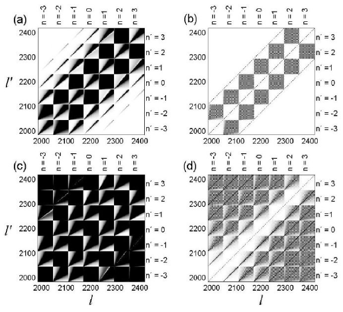
FIG. 1.: Central part of the Hamiltonian matrix. The $62\times 62$ blocks corresponding to $n,n^{\prime}=[-3,3]$ are shown. The larger the amplitudes of the matrix elements the more black the corresponding regions are. Four cases refer to: (a) one-cosine symmetric waveguide, (b) one-cosine asymmetric waveguide, (c) symmetric waveguide with a rough wall, $N_{T}=100$, (d) asymmetric waveguide with rough walls, $N_{T}=100$.

In order to analyze the structure of eigenstates of $\hat{H}$ in detail, we have diagonalized the Hamiltonian matrices shown in Fig.1 and constructed the ”state matrices” $|C^{\alpha}_{l}|^{2}$. Here $C^{\alpha}_{l}$ are the amplitudes of the eigenstates in the basis representaion given by the index $l$. Namely, the index $l$ refers to unperturbed basis states that correspond to the unperturbed Hamiltonian $\hat{H}^{0}$. The index $\alpha$ refers to a specific exact eigenstate. All eigenstes are reordered in increasing energy, with $\alpha=1$ the ground state. Therefore, to understand how strongly localized/extended are the exact eigenstates in the unperturbed basis, one should fix the value of $\alpha$ and explore the dependence of $|C^{\alpha}_{l}|^{2}$ on $l$.

Let us now compare the symmetric cases with the asymmetric ones, see Fig.2. The most important conclusion that can be deduced from the data is that the eigenstates are, in general, more extended in the asymmetric cases. Specifically, for the same small values of $\alpha$ there are more components $C^{\alpha}_{l}$ with large values of $l$, in comparison with the symmetric case, compare (c) with (d). At a first glance, this looks strange since for asymmetric profiles the Hamiltonian matrices are obviously less ”random” than for the symmetric ones, as is mentioned above. Close inspection of the data in Fig.2 shows that there is an additional effect that is also important in connection with the structure of eigenstates. Namely, the eigenstates for asymmetrical cases (b) and (d) turn out to be more sparse in comparison with the cases (a) and (c). This is manifested by a large number of ”holes” along each line in (b) and (d) for fixed values of $\alpha$, in the comparison with the cases (a) and (c). Thus, the eigenstates for waveguides with only gradient scattering (asymmetric case) are more extended in the unperturbed basis, and, at the same time, more sparse than for the wavegudies with both gradient and amplitude scattering (symmetric case).

This phenomenon is important in view of the scattering properties through waveguides of finite size with the profiles such as considered here. As is known, chaotic structure of eigenstates of closed (or periodic) waveguides/billiards is directly related to the scattering properties of open systems with the same profiles. For example, the degree of localization of eigenstates of closed systems determines the degree of localization of scattering states, and correspondingly, the value of transmission through open systems.

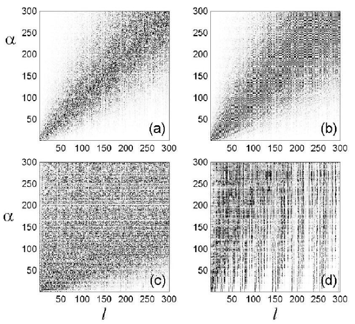
FIG. 2.: Lower part of the state matrix $|C^{\alpha}_{l}|^{2}$. The data for all cases (a-d) refer to the same profiles for which the structure of Hamiltonian matrices is shown in Fig.1. Here darker regions correspond to larger values of $|C^{\alpha}_{l}|^{2}$.

In conclusion, we have studied the structure of eigenstates of quasi-1D periodic waveguides with regular and random walls. Main attention was paid to the role of gradient scattering in comparison with the amplitude scattering. It was shown that for the case when the scattering walls have large number of harmonics, the gradient scattering itself is very strong. This is demonstrated by the data obtained for the waveguides with asymmetric walls, for which the amplitude scattering is absent. It was also revealed that the role of the gradient scattering is highly non-trivial. Specifically, the gradient scattering turns out to be relatively strong in the absence of the amplitude scattering.

We are grateful to N. Makarov for fruitful discussions. This work was supported by the CONACyT (Mexico) Grant No. 34668-E, and IIG3G02, VIEP, BUAP.

REFERENCES

- [1] Y.V. Fyodorov and A.D. Mirlin, Int. J. Mod. Phys. B, 8, 3795 (1994); K.B. Efetov, Supersymmetry in Disorder and Chaos (Cambridge University Press, Cambridge, England, 1997); A.D. Mirlin, Phys. Rep. 326, 259 (2000).
- [2] A. García-Martín, J.A. Torres, J.J. Sáenz, and M. Nieto-Vesperinas, Appl. Phys. Lett. 71, 1912 (1997); A. García-Martín, J.J. Sáenz, and M. Nieto-Vesperinas, Phys. Rev. Lett. 84, 3578 (2000).
- [3] J.A. Sánchez-Gil, V. Freilikher, I. Yurkevich, and A.A. Maradudin, Phys. Rev. B 59, 5915 (1999).
- [4] M. Leadbeater, V.I. Falko, and C.J. Lambert, Phys. Rev. Lett. 81, 1274 (1998).
- [5] F.M. Izrailev and N.M. Makarov, Phys. Rev. B 67, 113402 (2003).
- [6] G.A. Luna-Acosta, K. Na, L.E. Reichl, and A. Krokhin, Phys. Rev. E 53, 3271 (1996).
- [7] G.A. Luna-Acosta, J.A. Méndez-Bermúrdez, and F.M. Izrailev, Phys. Lett. A 274, 192 (2000); G.A. Luna-Acosta, J.A. Méndez-Bermúrdez, and F.M. Izrailev, Physica E 12, 267 (2002); Phys. Rev. E 65, 046605 (2002).
- [8] N. M. Makarov and Yu. V. Tarasov, J. Phys.: Condens. Matter, 10, 1523 (1998); N. M. Makarov, Yu. V. Tarasov, Phys. Rev. B, 64, 235306 (2001).
- [9] G.A. Luna-Acosta, A.A. Krokhin, M.A. Rodriguez, and P.H. Hernandez-Tejeda, Phys. Rev. B 54, 11410 (1996); G.A. Luna-Acosta, M.A. Rodriguez, A.A. Krokhin, K. Na, and R.A. Méndez, Rev. Mex. Fis. 44, S3 7 (1998); G.B. Akguc and L.E. Reichl, J. Stat. Phys. 98, 813 (2000); B. Huckestein, R. Ketzmerick, and C.H. Lewenkopf, Phys. Rev. Lett. 84, 5504 (2000); W. Li, L.E. Reichl, and B. Wu, Phys. Rev. E 65, 056220 (2002).
- [10] J.A. Méndez-Bermúrdez, G.A. Luna-Acosta, and F.M. Izrailev, to be published.