Interaction-induced magnetoresistance in a two-dimensional electron gas

Abstract

We study the interaction-induced quantum correction $\delta\sigma_{\alpha\beta}$ to the conductivity tensor of electrons in two dimensions for arbitrary $T\tau$ (where $T$ is the temperature and $\tau$ the transport scattering time), magnetic field, and type of disorder. A general theory is developed, allowing us to express $\delta\sigma_{\alpha\beta}$ in terms of classical propagators (“ballistic diffusons”). The formalism is used to calculate the interaction contribution to the longitudinal and the Hall resistivities in a transverse magnetic field in the whole range of temperature from the diffusive ($T\tau\ll 1$) to the ballistic ($T\tau\gtrsim 1$) regime, both in smooth disorder and in the presence of short-range scatterers. Further, we apply the formalism to anisotropic systems and demonstrate that the interaction induces novel quantum oscillations in the resistivity of lateral superlattices.

I Introduction

The magnetoresistance (MR) in a transverse field $B$ is one of the most frequently studied characteristics of the two-dimensional (2D) electron gas AA ; Been . Within the Drude-Boltzmann theory, the longitudinal resistivity of an isotropic degenerate system is $B$–independent,

$$\rho_{xx}(B)=\rho_{0}=(e^{2}\nu v_{F}^{2}\tau)^{-1},$$ (1.1)

where $\nu$ is the density of states per spin direction, $v_{F}$ the Fermi velocity, and $\tau$ the transport scattering time. Deviations from the constant $\rho_{xx}(B)$ are customarily called a positive or negative MR, depending on the sign of the deviation. There are several distinct sources of a non-trivial MR, which reflect the rich physics of the magnetotransport in 2D systems.

First of all, it has been recognized recently that even within the quasiclassical theory memory effects may lead to strong MR Hauge ; Baskin98 ; dmitriev01 ; FSDP ; PMR ; Antidots ; polyakov01 . The essence of such effects is that a particle “keeps memory” about the presence (or absence) of a scatterer in a spatial region which it has already visited. As a result, if the particle returns back, the new scattering event is correlated with the original one, yielding a correction to the resistivity (1.1). Since the magnetic field enhances the return probability, the correction turns out to be $B$-dependent. As a prominent example, memory effects in magnetotransport of composite fermions subject to an effective smooth random magnetic field explain a positive MR around half-filling of the lowest Landau level PMR . Another type of memory effects taking place in systems with rare strong scatterers is responsible for a negative MR in disordered antidot arrays Hauge ; Baskin98 ; dmitriev01 ; Antidots ; polyakov01 . However, such effects turn out to be of a relatively minor importance for the low–field quasiclassical magnetotransport in semiconductor heterostructures with typical experimental parameters, while at higher $B$ they are obscured by the development of the Shubnikov-de Haas oscillation (SdHO).

Second, the negative MR induced by the suppression of the quantum interference by the magnetic field is a famous manifestation of weak localization AA . While the weak-localization correction to conductivity is also related to the return probability, it has (contrary to the quasiclassical memory effects) an intrinsically quantum character, since it is governed by quantum interference of time-reversed paths. As a result it is suppressed already by a classically negligible magnetic field, which changes relative phases of the two paths. Consequently, the corresponding correction to $\rho_{xx}$ in high-mobility structures is very small and restricted to the range of very weak magnetic fields.

Finally, another quantum correction to MR is induced by the electron–electron interaction. While this effect is similar to those discussed above in its connection with the return probability (see Sec. IV below), it is distinctly different in several crucial aspects. In contrast to the memory effects, this contribution is of quantum nature and is therefore strongly $T$-dependent at low temperatures. On the other hand, contrary to the weak localization, the interaction correction to conductivity is not destroyed by a strong magnetic field. As a result, it induces an appreciable MR in the range of classically strong magnetic fields. This effect will be the subject of the present paper.

It was discovered by Altshuler and Aronov AA that the Coulomb interaction enhanced by the diffusive motion of electrons gives rise to a quantum correction to conductivity, which has in 2D the form (we set $k_{B}=\hbar=1$)

$$\delta\sigma_{xx}\simeq{e^{2}\over 2\pi^{2}}\left(1-{3\over 2}{\cal F}\right)\ln T\tau,\;\qquad T\tau\ll 1.$$ (1.2)

The first term in the factor $(1-{3\over 2}{\cal F})$ originates from the exchange contribution, and the second one from the Hartree contribution. In the weak-interaction regime, $\kappa\ll k_{F}$, where $\kappa=4\pi e^{2}\nu$ is the inverse screening length, the Hartree contribution is small, ${\cal F}\sim(\kappa/k_{F})\ln(k_{F}/\kappa)\ll 1$. The conductivity correction (1.2) is then dominated by the exchange term and is negative. The condition $T\tau\ll 1$ under which Eq. (1.2) is derived AA implies that electrons move diffusively on the time scale $1/T$ and is termed the “diffusive regime”. Subsequent works SenGir ; girvin82 showed that Eq. (1.2) remains valid in a strong magnetic field, leading (in combination with $\delta\sigma_{xy}=0$) to a parabolic interaction–induced quantum MR,

$${\delta\rho_{xx}(B)\over\rho_{0}}\simeq\left(1-{3\over 2}{\cal F}\right){{(\omega_{c}\tau)^{2}-1}\over\pi k_{F}l}\ln T\tau,\;\qquad T\tau\ll 1,$$ (1.3)

where $\omega_{c}=eB/mc$ is the cyclotron frequency and $l=v_{F}\tau$ the transport mean free path. Indeed, a $T$–dependent negative MR was observed in experiments PTH83 ; Choi ; Sav ; Minkov02 ; Minkov03 and attributed to the interaction effect. However, the majority of experiments PTH83 ; Choi ; Sav cannot be directly compared with the theory AA ; SenGir ; girvin82 since they were performed at higher temperatures, $T\tau\gtrsim 1$. (In high-mobility GaAs heterostructures conventionally used in MR experiments, $1/\tau$ is typically $\sim 100\ {\rm mK}$ and becomes even smaller with improving quality of samples.) In order to explain the experimentally observed $T$-dependent negative MR in this temperature range the authors of Refs. PTH83, ; Choi, conjectured various ad hoc extensions of Eq. (1.3) to higher $T$. Specifically, Ref. PTH83, conjectures that the logarithmic behavior (1.3) with $\tau$ replaced by the quantum time $\tau_{s}$ is valid up to $T\sim 1/\tau_{s}$, while Ref. Choi, proposes to replace $\ln T\tau$ by $-\pi^{2}/2T\tau$. These proposals, however, were not supported by theoretical calculations. There is thus a clear need for a theory of the MR in the ballistic regime, $T\gtrsim 1/\tau$.

In fact, the effect of interaction on the conductivity at $T\gtrsim 1/\tau$ has been already considered in the literature GD86 ; ZNA-sigmaxx ; ZNA-rhoxy ; ZNA-MRpar ; ZNA-deph ; reizer ; fluct-supercond . Gold and Dolgopolov GD86 analyzed the correction to conductivity arising from the $T$-dependent screening of the impurity potential. They obtained a linear-in-$T$ correction $\delta\sigma\sim e^{2}T\tau$. In the last few years, this effect attracted a great deal of interest in a context of low-density 2D systems showing a seemingly metallic behavior AKS01 ; Alt01 , $d\rho/dT>0$. Recently, Zala, Narozhny, and Aleiner ZNA-sigmaxx ; ZNA-rhoxy ; ZNA-MRpar developed a systematic theory of the interaction corrections valid for arbitrary $T\tau$. They showed that the temperature-dependent screening of Ref. GD86, has in fact a common physical origin with the Altshuler-Aronov effect but that the calculation of Ref. GD86, took only the Hartree term into account and missed the exchange contribution. In the ballistic range of temperatures, the theory of Refs. ZNA-sigmaxx, ; ZNA-rhoxy, ; ZNA-MRpar, , predicts, in addition to the linear-in-$T$ correction to conductivity $\sigma_{xx}$, a $1/T$ correction to the Hall coefficient ZNA-rhoxy $\rho_{xy}/B$ at $B\to 0$, and describes the MR in a parallel field ZNA-MRpar .

The consideration of Ref. ZNA-sigmaxx, ; ZNA-rhoxy, ; ZNA-MRpar, is restricted, however, to classically weak transverse fields, $\omega_{c}\tau\ll 1$, and to the white-noise disorder. The latter assumption is believed to be justified for Si-based and some (those with a very large spacer) GaAs structures, and the results of Refs. ZNA-sigmaxx, ; ZNA-rhoxy, ; ZNA-MRpar, have been by and large confirmed by most recent experiments Cole02 ; Shashkin02 ; proskuryakov02 ; kvon02 ; vitkalov02 ; pudalov02 ; noh02 on such systems. On the other hand, the random potential in typical GaAs heterostructures is due to remote donors and has a long–range character. Thus, the impurity scattering is predominantly of a small–angle nature and is characterized by two relaxation times, the transport time $\tau$ and the single-particle (quantum) time $\tau_{s}$ governing damping of SdHO, with $\tau\gg\tau_{s}$. Therefore, a description of the MR in such systems requires a more general theory valid also in the range of strong magnetic fields and for smooth disorder. [A related problem of the tunneling density of states in this situation was studied in Ref. RAG, .]

In this paper, we develop a general theory of the interaction–induced corrections to the conductivity tensor of 2D electrons valid for arbitrary temperatures, transverse magnetic fields, and range of random potential. We further apply it to the problem of magnetotransport in a smooth disorder at $\omega_{c}\tau\gg 1$. In the ballistic limit, $T\tau\gg 1$ (where the character of disorder is crucially important), we show that while the correction to $\rho_{xx}$ is exponentially suppressed for $\omega_{c}\ll T$, a MR arises at stronger $B$ where it scales as $B^{2}T^{-1/2}$. We also study the temperature-dependent correction to the Hall resistivity and show that it scales as $BT^{1/2}$ in the ballistic regime and for strong $B$. We further investigate a “mixed-disorder” model, with both short-range and long-range impurities present. We find that a sufficient concentration of short-range scatterers strongly enhances the MR in the ballistic regime.

The outline of the paper is as follows. In Sec. II we present our formalism and derive a general formula for the conductivity correction. We further demonstrate (Sec. II.3) that in the corresponding limiting cases our theory reproduces all previously known results for the interaction correction. In Sec. III we apply our formalism to the problem of interaction-induced MR in strong magnetic fields and smooth disorder. Section IV is devoted to a physical interpretation of our results in terms of a classical return probability. In Sections V and VI we present several further applications of our theory. Specifically, we analyze the interaction effects in systems with short-range scatterers and in magnetotransport in modulated systems (lateral superlattices). A summary of our results, a comparison with experiment, and a discussion of possible further developments is presented in Sec. VII. Some of the results of the paper have been published in a brief form in the Letter prl .

II General formalism

II.1 Smooth disorder

We consider a 2D electron gas (charge $-e$, mass $m$, density $n_{e}$) subject to a transverse magnetic field $B$ and to a random potential $u({\bf r})$ characterized by a correlation function

$$\langle u({\bf r})u({\bf r^{\prime}})\rangle=w(|{\bf r}-{\bf r^{\prime}}|)$$ (2.1)

with a spatial range $d$. The total ($\tau_{s}^{-1}$) and the transport ($\tau^{-1}$) scattering rates induced by the random potential are given by

$${1\over\tau_{s}} = 2\pi\nu\int_{0}^{2\pi}{d\phi\over 2\pi}W(\phi),$$ (2.2)

$${1\over\tau} = 2\pi\nu\int_{0}^{2\pi}{d\phi\over 2\pi}W(\phi)(1-\cos\phi),$$ (2.3)

where $W(\phi)=\tilde{w}(2k_{F}\sin{\phi\over 2})$ is the scattering cross-section. We begin by considering the case of smooth disorder, $k_{F}d\gg 1$, when $\tau/\tau_{s}\sim(k_{F}d)^{2}\gg 1$; generalization onto systems with arbitrary $\tau/\tau_{s}$ will be presented in Sec. II.2. We assume that the magnetic field is not too strong, $\omega_{c}\tau_{s}\ll 1$, so that the Landau quantization is destroyed by disorder. Note that this assumption is not in conflict with a condition of classically strong magnetic fields ($\omega_{c}\tau\gg 1$), which is a range of our main interest in the present paper.

We consider two types of the electron-electron interaction potential $U_{0}({\bf r})$: (i) point-like interaction, $U_{0}({\bf r})=V_{0}$, and (ii) Coulomb interaction, $U_{0}({\bf r})=e^{2}/r$. In order to find the interaction-induced correction $\delta\sigma_{\alpha\beta}$ to the conductivity tensor, we make use of the “ballistic” generalization of the diffuson diagram technique of Ref. AA, . We consider the exchange contribution first and will discuss the Hartree term later on. Within the Matsubara formalism, the conductivity is expressed via the Kubo formula through the current-current correlation function,

$$\sigma_{\alpha\beta}(i\Omega_{k})={n_{e}e^{2}\over m\Omega_{k}}\delta_{\alpha\beta}$$

$$-{1\over\Omega_{k}}\int_{0}^{1/T}\!\!d\tau\int d^{2}r\langle{{\cal T}_{\tau}\hat{j}_{\alpha}({\bf r},\tau)}{\hat{j}_{\beta}(0,0)}\rangle e^{i\Omega_{k}\tau},$$

(2.4)

where $\Omega_{k}=2\pi kT$ is the bosonic Matsubara frequency. Diagrams for the leading-order interaction correction are shown in Fig. 1 and can be generated in the following way. First, there are two essentially different ways to insert an interaction line into the bubble formed by two electronic Green’s function. Second, one puts signs of electronic Matsubara frequencies in all possible ways. On the third step, one connects lines with opposite signs of frequencies $\epsilon_{n}>0,\ \epsilon_{m}<0$ by impurity–line ladders (which are not allowed to cross each other). Finally, in the case of the diagram a, where four electronic lines form a “box”, one should include two additional diagrams, b and c, with an extra impurity line (“Hikami box”).

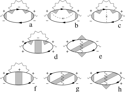
Figure 1: Exchange diagrams for the interaction correction to $\sigma_{\alpha\beta}$. The wavy (dashed) lines denote the interaction (impurity scattering), the shaded blocks are impurity ladders, and the $+/-$ symbols denote the signs of the Matsubara frequencies. The diagrams obtained by a flip and/or by an exchange $+\leftrightarrow-$ should also be included. “Inelastic” part of the diagrams f, g is canceled by a contribution of the Coulomb-drag type, see Appendix A.

The impurity–line ladders are denoted by shaded blocks in Fig. 1; we term them “ballistic diffusons”. Formally, the ballistic diffuson is defined as an impurity average (denoted below as $\langle\dots\rangle_{\rm imp}$) of a product of a retarded and advanced Green’s functions,

$${\cal D}(i\epsilon_{m},i\epsilon_{n};{\bf r}_{1},{\bf r}_{2};{\bf r}_{3},{\bf r}_{4})$$

$$=\theta(-\epsilon_{m}\epsilon_{n})\langle G({\bf r}_{1},{\bf r}_{2};i\epsilon_{m})G({\bf r}_{3},{\bf r}_{4};i\epsilon_{n})\rangle_{\rm imp}.$$

(2.5)

Following the standard route of the quasiclassical formalism semi ; AL ; RAG-dos-corr , we perform the Wigner transformation,

$${\cal D}(i\epsilon_{m}-i\epsilon_{n};{\bf R}_{1},{\bf p}_{1};{\bf R}_{2},{\bf p}_{2})=\int d{\bf r}d{\bf r}^{\prime}$$

$$\times e^{-i[{\bf p}_{1}-(e/c)\bf A(\bf R_{1})]{\bf r}}e^{-i[{\bf p}_{2}-(e/c)\bf A(\bf R_{2})]{\bf r}^{\prime}}$$

$$\times{\cal D}(i\epsilon_{m},i\epsilon_{n};{\bf R}_{1},{\bf r};{\bf R}_{2},{\bf r}^{\prime}),$$ (2.6)

where ${\bf R}_{1}=({\bf r}_{4}+{\bf r}_{1})/2$, ${\bf R}_{2}=({\bf r}_{2}+{\bf r}_{3})/2$, ${\bf r}={\bf r}_{4}-{\bf r}_{1}$, and ${\bf r}^{\prime}={\bf r}_{2}-{\bf r}_{3}$. Note that the factors depending on the vector potential make the ballistic diffuson (2.6) gauge-invariant. Finally, we integrate out the absolute values of momenta $p_{1,2}$ and get the final form of the ballistic diffuson

$${\cal D}(i\omega_{l};{\bf R}_{1},{\bf n}_{1};{\bf R}_{2},{\bf n}_{2})$$

$$={1\over 2\pi\nu}\int{p_{1}dp_{1}\over 2\pi}\int{p_{2}dp_{2}\over 2\pi}{\cal D}(i\omega_{l};{\bf R}_{1},{\bf p}_{1};{\bf R}_{2},{\bf p}_{2}),$$

(2.7)

which describes the quasiclassical propagation of an electron in the phase space from the point ${\bf R}_{2},{\bf n}_{2}$ to ${\bf R}_{1},{\bf n}_{1}$. Here ${\bf n}$ is the unit vector characterizing the direction of velocity on the Fermi surface. The ballistic diffuson satisfies the quasiclassical Liouville-Boltzmann equation

$$\left[|\omega_{l}|+iv_{F}q\cos(\phi-\phi_{q})+\omega_{c}{\partial\over\partial\phi}\right. + \left.{\hat{C}}\right]{\cal D}(i\omega_{l},{\bf q};\phi,\phi^{\prime})$$ (2.8)

$$= 2\pi\delta(\phi-\phi^{\prime}),$$

where $\phi\ (\phi_{q})$ is the polar angle of ${\bf n}\ ({\bf q})$ and ${\hat{C}}$ is the collision integral, determined by the scattering cross-section $W({\bf n},{\bf n^{\prime}}).$ For the case of a smooth disorder, the collision integral is given by

$${\hat{C}}=-{1\over\tau}{\partial^{2}\over\partial\phi^{2}}.$$ (2.9)

In contrast to the diffusive regime, where ${\cal D}$ has a universal and simple structure ${\cal D}(i\omega_{l},{\bf q})=1/(Dq^{2}+|\omega_{l}|)$ determined by the diffusion constant $D$ only, its form in the ballistic regime is much more complicated. We are able, however, to get a general expression for $\delta\sigma_{\alpha\beta}$ in terms of the ballistic propagator ${\cal D}(\omega_{l},{\bf q};{\bf n},{\bf n}^{\prime})$.

The temperature range of main interest in the present paper is restricted by $T\tau_{s}\ll 1$, since at higher $T$ the MR will be small in the whole range of the quasiclassical transport $\omega_{c}\tau_{s}\ll 1$ (see below). In this case the ladders are dominated by contributions with many ($\gg 1$) impurity lines. We will assume this situation when evaluating diagrams in the present subsection. A general case of arbitrary $T\tau_{s}$ and $\tau_{s}/\tau$ will be addressed in Sec. II.2.

Figure 2: Diagrams obtained by a flip and/or by an exchange $+\leftrightarrow-$ from the diagram d.

We start with the diagrams d and e that give rise to the logarithmic correction in the diffusive regime AA . Let us fix the sign of the external frequency, $\Omega_{k}>0.$ Each of the diagrams d and e generates four diagrams by a flip with respect to the horizontal line or by exchange $+\leftrightarrow-$, see Fig. 2. Consider first the diagram $d_{++}$. There are two triangular boxes containing each a current vertex and three electron Green’s functions (Fig. 3). In the quasiclassical regime $\omega_{c}\tau_{s}\ll 1$ one may neglect the effect of magnetic field on the Green’s functions (keeping $\omega_{c}$ in the ballistic propagators only). Furthermore, using $T\tau_{s}\ll 1$, we neglect the difference in momenta and frequencies in the Green’s functions, since typical values of frequencies $i\Omega_{k}$, $i\omega_{l}$ and momenta ${\bf q}$ carried by the ballistic diffusons are set by the temperature. Each triangle then reads

$$\Gamma_{\alpha}({\bf n}) = {e\over m}\int{pdp\over 2\pi}{p\ n_{\alpha}\over(-\xi_{p}+i/2\tau_{s})^{2}(-\xi_{p}-i/2\tau_{s})}$$ (2.10)

$$\simeq i2\pi\nu\tau_{s}^{2}ev_{F}n_{\alpha},$$

where $\xi_{p}=p^{2}/2m-\mu$. Combining the triangles with the three ballistic propagators separated by the impurity lines (see Fig. 3), we obtain the following expression for the electronic part of the diagram $d_{++}$,

$$(2\pi\nu)^{3}\int\prod_{i=1}^{6}{d\phi_{i}\over 2\pi}{\cal D}(i\omega_{l},{\bf q};\phi,\phi_{1})W(\phi_{1}-\phi_{2})\Gamma_{\alpha}(\phi_{2})$$

$$\times W(\phi_{2}-\phi_{3}){\cal D}(i\omega_{l}-i\Omega_{k},{\bf q};\phi_{3},\phi_{4})W(\phi_{4}-\phi_{5})$$

$$\times\Gamma_{\beta}(\phi_{5})W(\phi_{5}-\phi_{6}){\cal D}(i\omega_{l},{\bf q};\phi_{6},\phi^{\prime})$$

$$\equiv{4\pi\sigma_{0}\over\tau}{\cal B}^{d}_{\alpha\beta}(i\omega_{l},-i\Omega_{k},{\bf q};\phi,\phi^{\prime}).$$ (2.11)

In what follows we will use for brevity a short-hand notation

$$(2\pi\nu)^{3}{\cal D}W\Gamma_{\alpha}W{\cal D}W\Gamma_{\beta}W{\cal D}$$

for the l.h.s. of (2.11) and analogous notations for other structures of this type. Making use of the small-angle nature of scattering in a smooth random potential, we can replace the $W(\phi_{i}-\phi_{j})$ factors in (2.11) by $(\nu\tau_{s})^{-1}\delta(\phi_{i}-\phi_{j})$, yielding

$${\cal B}^{d}_{\alpha\beta}(q,i\omega_{l},i\Omega_{k};\phi,\phi^{\prime})$$

$$\simeq-{\cal D}(i\omega_{l},{\bf q})n_{\alpha}{\cal D}(i\omega_{l}+i\Omega_{k},{\bf q})n_{\beta}{\cal D}(i\omega_{l},{\bf q}).$$

In the exchange term (calculated in the present subsection) this structure is further integrated over the angles $\phi$ and $\phi^{\prime}$,

$$B^{d}_{\alpha\beta}(i\omega_{l},i\Omega_{k},{\bf q})=\langle{\cal B}^{d}_{\alpha\beta}(i\omega_{l},i\Omega_{k},{\bf q};\phi,\phi^{\prime})\rangle.$$ (2.12)

The angular brackets $\langle\dots\rangle$ denote averaging over velocity directions, e.g.

$$\langle n_{x}{\cal D}n_{x}\rangle\equiv\int{d\phi_{1}\over 2\pi}{d\phi_{2}\over 2\pi}\cos\phi_{1}{\cal D}(\omega_{l},{\bf q};\phi_{1},\phi_{2})\cos\phi_{2}.$$

The fermionic frequencies obey the inequalities $\epsilon_{m}>0$, $\epsilon_{m}-\omega_{l}<0$, and $\epsilon_{m}-\Omega_{k}>0$, which implies $\omega_{l}>\epsilon_{m}>\Omega_{k}$, so that the summation over $\epsilon_{m}$ gives the factor $(\omega_{l}-\Omega_{k})/2\pi T$.

Figure 3: Diagram $d$ drawn in a different way in order to visualize the structure of Eq. (2.11). The dashed frame encloses the electronic part ${\cal B}_{\alpha\beta}^{d}$.

The diagram $d_{--}$ has the same structure (both triangles have opposite signs, thus the total sign remains unchanged), but the frequency summation is restricted by $\epsilon_{m}<0$, $\epsilon_{m}-\omega_{l}>0$, and $\epsilon_{m}-\Omega_{k}<0$, yielding the factor $-\omega_{l}/2\pi T$ in the conductivity correction. The diagrams $d^{\prime}_{++}$ and $d^{\prime}_{--}$ obtained from $d_{++}$ and $d_{--}$ by a flip (or, equivalently, by reversing all arrows) double the result. Combining the four contributions and changing sign of the summation variable, $\omega_{l}\to-\omega_{l}$ in $d_{--}$ and $d^{\prime}_{--}$ terms, we have

$$\delta\sigma_{\alpha\beta}^{d}(i\Omega_{k})=-{8\pi\sigma_{0}\over\tau}{T^{2}\over\Omega_{k}}\int{d^{2}q\over(2\pi)^{2}}$$

$$\times\left[\ \sum_{\omega_{l}>\Omega_{k}}{\omega_{l}-\Omega_{k}\over 2\pi T}U(i\omega_{l},{\bf q})B^{d}_{\alpha\beta}(-i\omega_{l},i\Omega_{k},{\bf q})\right.$$

$$+\left.\sum_{\omega_{l}>0}{\omega_{l}\over 2\pi T}U(i\omega_{l},{\bf q})B^{d}_{\alpha\beta}(i\omega_{l},i\Omega_{k},{\bf q})\ \right],$$ (2.13)

where $U(i\omega,{\bf q})$ is the interaction potential equal to a constant $V_{0}$ for point-like interaction and to

$$U(i\omega_{l},{\bf q})=\frac{1}{2\nu}\ \frac{\kappa}{q+\kappa[1-|\omega_{l}|\langle{\cal D}({\bf q},i\omega_{l})\rangle]}$$ (2.14)

for screened Coulomb interaction. In (2.13) we used the fact that $U({\bf q},-i\omega_{l})=U({\bf q},i\omega_{l})$ and ${\cal D}({\bf q},-i\omega_{l})={\cal D}({\bf q},i\omega_{l})$. Equation (2.14) is a statement of the random-phase approximation (RPA), with the polarization operator given by

$$\Pi(i\omega_{l},{\bf q})=2\nu[1-|\omega_{l}|\langle{\cal D}(i\omega_{l},{\bf q})\rangle].$$ (2.15)

The first term (unity) in square brackets in (2.15) comes from the $++$ and $--$ contributions to the polarization bubble, while the second term is generated by the $+-$ contribution (ballistic diffuson).

The diagrams e are evaluated in a similar way. In all four diagrams of this type one of the electron triangles is the same as in diagrams d while another one has an opposite sign. The structures arising after integrating out fast momenta in electron bubbles coincide with those of d-type ($B_{\alpha\beta}^{d}$). Summation over the fermionic frequency $\epsilon_{m}$ is constrained by the condition $\omega_{l}>\epsilon_{m}>\Omega_{k}$ for all the $e$-type diagrams. The correction due to the diagrams e therefore reads

$$\delta\sigma_{\alpha\beta}^{e}(i\Omega_{k})={8\pi\sigma_{0}\over\tau}{T^{2}\over\Omega_{k}}\int\!\!{d^{2}q\over(2\pi)^{2}}\sum_{\omega_{l}>\Omega_{k}}\!\!\!{\omega_{l}-\Omega_{k}\over 2\pi T}\>U(i\omega_{l},{\bf q})$$

$$\times\left[B^{d}_{\alpha\beta}(-i\omega_{l},i\Omega_{k},{\bf q})+B^{d}_{\alpha\beta}(i\omega_{l},i\Omega_{k},{\bf q})\right].$$ (2.16)

We see that the first term in square brackets in (2.16) cancels the first term in (2.13). Thus, the sum of the contributions of diagrams d and e takes the form

$$\delta\sigma_{\alpha\beta}^{d+e}(i\Omega_{k}) = -{4\sigma_{0}\over\tau}{T\over\Omega_{k}}\left[\sum_{\omega_{l}=0}^{\Omega_{k}}\omega_{l}\Phi^{d}_{\alpha\beta}(i\omega_{l},i\Omega_{k})\right.$$ (2.17)

$$+ \left.\sum_{\omega_{l}>\Omega_{k}}\Omega_{k}\Phi^{d}_{\alpha\beta}(i\omega_{l},i\Omega_{k})\right],$$

where we introduced a notation

$$\Phi^{\mu}_{\alpha\beta}(i\omega_{l},i\Omega_{k})=\int{d^{2}q\over(2\pi)^{2}}U(i\omega_{l},{\bf q})B^{\mu}_{\alpha\beta}(i\omega_{l},i\Omega_{k},{\bf q}),$$ (2.18)

with the index $\mu$ labeling the diagram.

Similarly, we obtain for the diagram h

$$\delta\sigma_{\alpha\beta}^{h}(i\Omega_{k}) = -{4\sigma_{0}\over\tau}{T\over\Omega_{k}}\left[\sum_{\omega_{l}=0}^{\Omega_{k}}\omega_{l}\Phi^{h}_{\alpha\beta}(i\omega_{l},i\Omega_{k})\right.$$ (2.19)

$$+ \left.\sum_{\omega_{l}>\Omega_{k}}\Omega_{k}\Phi^{h}_{\alpha\beta}(i\omega_{l},i\Omega_{k})\right],$$

with

$$B^{h}_{\alpha\beta}(i\omega_{l},i\Omega_{k},{\bf q})=-2T_{\alpha\gamma}\langle n_{\gamma}{\cal D}(i\omega_{l}+i\Omega_{k},{\bf q})n_{\beta}{\cal D}(i\omega_{l},{\bf q})\rangle.\\$$

The tensor $T_{\alpha\gamma}$ appearing in (II.1) describes the renormalization of a current vertex connecting two electronic lines with opposite signs of frequencies,

$$T_{\alpha\beta} = 2\left.\langle n_{\alpha}{\cal D}n_{\beta}\rangle\right|_{q=0,\omega\to 0}={\sigma_{\alpha\beta}\over e^{2}v_{F}^{2}\nu}$$ (2.22)

$$= {\tau\over 1+\omega_{c}^{2}\tau^{2}}\left(\begin{array}[]{cc}1&-\omega_{c}\tau\\ \omega_{c}\tau&1\end{array}\right).$$

We turn now to diagrams f and g. The expressions for the corresponding contributions read

$$\delta\sigma_{\alpha\beta}^{f}(i\Omega_{k})=-{4\sigma_{0}\over\tau}{T\over\Omega_{k}}\left[\sum_{\omega_{l}\geq 0}\Omega_{k}\Phi^{f}_{\alpha\beta}(i\omega_{l},i\Omega_{k})\right.$$

$$+\left.\sum_{-\Omega_{k}<\omega_{l}<0}\!\!(\Omega_{k}+\omega_{l})\Phi^{f}_{\alpha\beta}(-i\omega_{l},i\Omega_{k})\right],$$ (2.23)

$$\delta\sigma_{\alpha\beta}^{g}(i\Omega_{k})={4\sigma_{0}\over\tau}{T\over\Omega_{k}}\left[\sum_{\omega_{l}=0}^{\Omega_{k}}(\Omega_{k}-\omega_{l})\Phi^{f}_{\alpha\beta}(i\omega_{l},i\Omega_{k})\right.$$

$$+\left.\sum_{-\Omega_{k}<\omega_{l}<0}\!\!(\Omega_{k}+\omega_{l})\Phi^{f}_{\alpha\beta}(-i\omega_{l},i\Omega_{k})\right],$$ (2.24)

with

$$B^{f}_{\alpha\beta}(i\omega_{l},i\Omega_{k},{\bf q})=T_{\alpha\gamma}\langle n_{\gamma}{\cal D}(i\omega_{l}+i\Omega_{k},{\bf q})n_{\delta}\rangle T_{\delta\beta}.\\$$

The sum of the contributions f and g is therefore given by

$$\delta\sigma_{\alpha\beta}^{f+g}(i\Omega_{k}) = -{4\sigma_{0}\over\tau}{T\over\Omega_{k}}\left[\sum_{\omega_{l}=0}^{\Omega_{k}}\omega_{l}\Phi^{f}_{\alpha\beta}(i\omega_{l},i\Omega_{k})\right.$$ (2.25)

$$+ \left.\sum_{\omega_{l}>\Omega_{k}}\Omega_{k}\Phi^{f}_{\alpha\beta}(i\omega_{l},i\Omega_{k})\right].$$

We see that when the diagrams ${\it f}$ and ${\it g}$ are combined, the same Matsubara structure as for other diagrams [Eqs. (2.17), (2.19)] arises. In other words, the role of the diagrams g is to cancel the extra contribution of diagrams f, which has a different Matsubara structure.

A word of caution is in order here. In our calculation we have set the value of velocity coming from current vertices to be equal $v_{F}$, thus neglecting a particle-hole asymmetry. If one goes beyond this approximation and takes into account the momentum-dependence of velocity (violating the particle-hole symmetry), the above cancellation ceases to be exact and an additional term with a different Matsubara structure arises in $\delta\sigma_{\alpha\beta}^{f+g}$. After the analytical continuation is performed, the corresponding correction to the conductivity has a form

$$\delta\sigma^{\rm inel}_{\alpha\beta} = -{2\sigma_{0}\over\tau}\int_{-\infty}^{\infty}{d\omega\over 2\pi}{\omega\over 2T\sinh^{2}(\omega/2T)}$$ (2.26)

$$\times \!\!\int{d^{2}q\over(2\pi)^{2}}\ \delta B^{f}_{\alpha\beta}(\omega,q)\ {\rm Im}\,U(\omega,q),$$

characteristic for effects governed by inelastic scattering. This contribution is determined by real inelastic scattering processes with an energy transfer $\omega\lesssim T$ and behaves (in zero magnetic field) as $e^{2}(T\tau)^{2}$. This implies that the corresponding resistivity correction, $\delta\rho\sim(T/eE_{F})^{2}$ is independent of disorder. However, such a correction should not exist because of total momentum conservation. Indeed, an explicit calculation (see Appendix A) shows that this term is canceled by the Aslamazov-Larkin-type diagrams analogous to those describing the Coulomb drag.

Finally, we consider the diagrams a,b, and c. Already taken separately, each of them has the expected Matsubara structure (contrary to the diagrams d,e and f,g, which should be combined to get this structure). However, another peculiarity should be taken into account. The diagrams a,b, and c form together the Hikami box, so that their sum is smaller by a factor $\sim\tau_{s}/\tau$ than separate terms. Therefore, some care is required: subleading terms of order $\tau_{s}/\tau$ should be retained when contributions of individual diagrams are calculated. The result reads

$$\delta\sigma_{\alpha\beta}^{a+b+c}(i\Omega_{k}) = -{4\sigma_{0}\over\tau}{T\over\Omega_{k}}\left[\sum_{\omega_{l}=0}^{\Omega_{k}}\omega_{l}\Phi^{a+b+c}_{\alpha\beta}(i\omega_{l},i\Omega_{k})\right.$$ (2.27)

$$+ \left.\sum_{\omega_{l}>\Omega_{k}}\Omega_{k}\Phi^{a+b+c}_{\alpha\beta}(i\omega_{l},i\Omega_{k})\right].$$

Here the contributions of individual diagrams a, b, and c have the form

$$B^{a}_{\alpha\beta}(i\omega_{l},i\Omega_{k},{\bf q})$$

$$={1\over 2}T_{\alpha\gamma}\left[{1\over\tau_{s}}\delta_{\gamma\delta}+({\tilde{T}}^{-1})_{\gamma\delta}\right]T_{\delta\beta}\langle{\cal D}(i\omega_{l},{\bf q}){\cal D}(i\omega_{l},{\bf q})\rangle$$

$$+{1\over 2}T_{\alpha\gamma}T_{\gamma\beta}\langle{\cal D}(i\omega_{l},{\bf q})\rangle,$$ (2.28)

where the matrix ${\tilde{T}}_{\alpha\beta}$ has the same form as $T_{\alpha\beta}$ with a replacement $\tau\to\tau_{s}$,

$$B^{b}_{\alpha\beta}(i\omega_{l},i\Omega_{k},{\bf q})=-{1\over 2\tau_{s}}T_{\alpha\gamma}T_{\gamma\beta}\langle{\cal D}(i\omega_{l},{\bf q}){\cal D}(q,i\omega_{l})\rangle,$$ (2.29)

and

$$B^{c}_{\alpha\beta}(i\omega_{l},i\Omega_{k},{\bf q})=$$

$$-{1\over 2}\left({1\over\tau_{s}}-{1\over\tau}\right)T_{\alpha\gamma}T_{\gamma\beta}\langle{\cal D}(i\omega_{l},{\bf q}){\cal D}(i\omega_{l},{\bf q})\rangle.$$

(2.30)

We see that although each of the expressions (II.1), (2.29), and (2.30) depends on $\tau_{s}$, the single-particle time disappears from the total contribution of the Hikami-box,

$$B^{a+b+c}_{\alpha\beta}(i\omega_{l},i\Omega_{k},{\bf q}) = {1\over 2}T_{\alpha\beta}\langle{\cal D}(i\omega_{l},{\bf q}){\cal D}(i\omega_{l},{\bf q})\rangle$$ (2.31)

$$+ {1\over 2}T_{\alpha\gamma}\langle{\cal D}(i\omega_{l},{\bf q})\rangle T_{\gamma\beta}.$$

The total correction to the conductivity tensor is obtained by collecting the contributions (2.17), (2.19), (2.25), and (2.27). Carrying out the analytical continuation to real frequencies, we get

$$\delta\sigma_{\alpha\beta}(\Omega) = {\sigma_{0}\over i\pi\tau\Omega}\int_{-\infty}^{\infty}d\omega\,\omega\coth{\omega\over 2T}$$ (2.32)

$$\times [\Phi_{\alpha\beta}(\omega+\Omega,\Omega)-\Phi_{\alpha\beta}(\omega,\Omega)],$$

where

$$\Phi_{\alpha\beta}(\omega,\Omega) = \Phi^{a+b+c}_{\alpha\beta}(\omega,\Omega)+\Phi^{d}_{\alpha\beta}(\omega,\Omega)$$ (2.33)

$$+ \Phi^{f}_{\alpha\beta}(\omega,\Omega)+\Phi^{h}_{\alpha\beta}(\omega,\Omega).$$

We are interested in the case of zero external frequency, $\Omega\to 0$, when Eq. (2.32) can be rewritten as

$$\delta\sigma_{\alpha\beta} = -{\sigma_{0}\over i\pi\tau}\int_{-\infty}^{\infty}d\omega$$ (2.34)

$$\times \Phi_{\alpha\beta}(\omega,0){\partial\over\partial\omega}\left[\omega\coth{\omega\over 2T}\right].$$

Recalling the definition (2.18) of $\Phi^{\mu}$, we finally arrive at the following result

$$\delta\sigma_{\alpha\beta} = -2e^{2}v_{F}^{2}\nu\int_{-\infty}^{\infty}\frac{d\omega}{2\pi}\frac{\partial}{\partial\omega}\left[\omega\ \coth{\omega\over{2T}}\right]$$

$$\times \int\frac{d^{2}{\bf q}}{(2\pi)^{2}}\ {\rm Im}\left[\ U(\omega,{\bf q})\ B_{\alpha\beta}(\omega,{\bf q})\ \right],$$

where the tensor $B_{\alpha\beta}(\omega,{\bf q})$ is given by

$$B_{\alpha\beta}(\omega,{\bf q}) = {T_{\alpha\beta}\over 2}\langle{\cal D}{\cal D}\rangle+T_{\alpha\gamma}\!\left({\delta_{\gamma\delta}\over 2}\langle{\cal D}\rangle-\langle n_{\gamma}{\cal D}n_{\delta}\rangle\right)\!T_{\delta\beta}$$ (2.36)

$$- 2T_{\alpha\gamma}\langle n_{\gamma}{\cal D}n_{\beta}{\cal D}\rangle-\langle{\cal D}n_{\alpha}{\cal D}n_{\beta}{\cal D}\rangle.$$

The first term in (2.36) originates from the diagrams a,b,c, the second term from a,f,g, the third term from h, and the last one – from d and e. We remind the reader that this result has been obtained under the assumption $\tau_{s}\ll\tau,\>T^{-1}$; generalization to arbitrary $\tau_{s}/\tau$ and $\tau_{s}T$ will be considered in Sec. II.2. It will be shown there that the conductivity correction retains the form (LABEL:sigma) in the general case but the expression (2.36) for $B_{\alpha\beta}(\omega,{\bf q})$ is slightly modified.

II.2 General case

In the previous subsection we have derived the formula for the correction to the conductivity tensor for the case of a smooth disorder (with $\tau_{s}\ll\tau$) assuming $\tau_{s}\ll T^{-1}$. Since characteristic momenta $q$ and frequencies $\omega$ are set by the temperature, this assumption implies $ql_{s}\ll 1$ and $\omega\tau_{s}\ll 1$. This allowed us to simplify the calculation by neglecting the $q$ and $\omega$ dependence of Green’s functions connecting ballistic diffusons and by considering only the ladders with many impurity lines. Furthermore, we have used the small-angle nature of scattering when calculating the Hikami box contribution (2.31). We are now going to discuss the general case of arbitrary $\tau_{s}/\tau$ and $T\tau_{s}$.

It turns out that the expressions (2.17), (2.19), and (2.25) for the contribution of the diagrams $d-h$ derived in the case of a smooth disorder remain valid in the general situation. The simplest way to show this is to use the following technical trick (cf. Refs. bmm01, ; gm02, ). One can add to the system an auxiliary weak smooth random potential with a long transport scattering time $\tilde{\tau}\gg\tau$ but short single-particle ${\tilde{\tau}}_{s}\ll\tau_{s}$, such that $T{\tilde{\tau}}_{s}\ll 1$. This potential will not affect the quasiclassical dynamics and thus should not change the result. On the other hand, it allows us (in view of the condition $T{\tilde{\tau}}_{s}\ll 1$) to perform the gradient and frequency expansion in Green’s functions as was done in Sec. II.1. Adding such an auxiliary disorder amounts to a re-distribution between quantum and quasiclassical degrees of freedom: all the information about the real disorder is now contained in the ballistic propagators. It can be verified by a direct calculation (without using the additional disorder) that the above procedure yields the correct result.

It remains to consider the Hikami-box contribution (2.27). When calculating it in Sec. II.1, we used the small-angle nature of scattering implying that a single scattering line inserted between two ballistic propagators approximately preserves the direction of velocity, $\langle{\cal D}W{\cal D}\rangle\to(2\pi\nu)^{-1}\langle{\cal D}{\cal D}\rangle/\tau_{s}$ and $\langle{\cal D}n_{\alpha}Wn_{\beta}{\cal D}\rangle\to(2\pi\nu)^{-1}\langle{\cal D}{\cal D}\rangle(1/\tau_{s}-1/\tau)\delta_{\alpha\beta}$. In the more general situation, when the scattering is at least partly of the large–angle character, this is no longer valid and Eq. (2.31) acquires a slightly more complicated form,

$$B^{a+b+c}_{\alpha\beta}({\bf q},i\omega_{l},i\Omega_{k})=$$

$$\pi\nu T_{\alpha\gamma}[\langle{\cal D}{\cal S}_{\gamma\delta}{\cal D}\rangle-2\langle{\cal D}n_{\gamma}Wn_{\delta}{\cal D}\rangle]T_{\delta\beta}$$

$$+{1\over 2}T_{\alpha\gamma}\langle{\cal D}\rangle T_{\gamma\beta},$$ (2.37)

where ${\cal S}_{xx}={\cal S}_{yy}=W({\bf n},{\bf n^{\prime}}),\quad{\cal S}_{xy}=-{\cal S}_{yx}=\omega_{c}/2\pi\nu$.

Summarizing the consideration in this subsection, in the general situation the interaction correction retains the form (LABEL:sigma) with the tensor $B_{\alpha\beta}(\omega,{\bf q})$ given by

$$B_{\alpha\beta}(\omega,{\bf q})=T_{\alpha\gamma}\pi\nu[\langle{\cal D}{\cal S}_{\gamma\delta}{\cal D}\rangle-2\langle{\cal D}n_{\gamma}Wn_{\delta}{\cal D}\rangle]T_{\delta\beta}$$

$$+T_{\alpha\gamma}\left({\delta_{\gamma\delta}\over 2}\langle{\cal D}\rangle-\langle n_{\gamma}{\cal D}n_{\delta}\rangle\right)T_{\delta\beta}$$

$$-2T_{\alpha\gamma}\langle n_{\gamma}{\cal D}n_{\beta}{\cal D}\rangle-\langle{\cal D}n_{\alpha}{\cal D}n_{\beta}{\cal D}\rangle.$$ (2.38)

The correction $\delta\rho_{\alpha\beta}$ to the resistivity tensor is then immediately obtained by using $\delta\hat{\rho}=-\hat{\rho}\,\delta\hat{\sigma}\,\hat{\rho}$. This yields

$$\delta\rho_{\alpha\beta} = {2\over e^{2}v_{F}^{2}\nu}\int_{-\infty}^{\infty}\frac{d\omega}{2\pi}\frac{\partial}{\partial\omega}\left[\omega\ {\rm coth}{\omega\over{2T}}\right]$$

$$\times \int\frac{d^{2}{\bf q}}{(2\pi)^{2}}\ {\rm Im}\left[\ U(\omega,{\bf q})\ B^{(\rho)}_{\alpha\beta}(\omega,{\bf q})\ \right],$$

where the tensor $B^{(\rho)}_{\alpha\beta}$ is related to $B_{\alpha\beta}$, Eq. (II.2), via

$$B^{(\rho)}_{\alpha\beta}=(T^{-1})_{\alpha\gamma}B_{\gamma\delta}(T^{-1})_{\delta\beta}.$$ (2.40)

Explicitly, corrections to the components of the resistivity tensor are expressed through $\delta\sigma_{xx}=\delta\sigma_{yy}$ and $\delta\sigma_{xy}=-\delta\sigma_{yx}$ as follows

$$\delta\rho_{xx} = \rho_{0}^{2}[(\omega_{c}^{2}\tau^{2}-1)\delta\sigma_{xx}+2\omega_{c}\tau\delta\sigma_{xy}],$$ (2.41)

$$\delta\rho_{xy} = \rho_{0}^{2}[(\omega_{c}^{2}\tau^{2}-1)\delta\sigma_{xy}-2\omega_{c}\tau\delta\sigma_{xx}].$$ (2.42)

Note that the results (2.36), (II.2) for $B_{\alpha\beta}(\omega,{\bf q})$ satisfy the requirement

$$B_{\alpha\beta}(\omega,0)=0,$$ (2.43)

as follows from

$$\left.\langle n_{\alpha}{\cal D}n_{\beta}\rangle\right|_{q=0}=\sigma_{\alpha\beta}(\omega)/2e^{2}\nu v_{F}^{2}$$

and $\left.(2\pi)^{-1}\!\int d\phi\ {\cal D}(\phi,\phi^{\prime})\right|_{q=0}=i/\omega.$ The condition (2.43) implies that spatially homogeneous fluctuations in the potential do not change the conductivity, see Refs. ZNA-sigmaxx, ,Ka-And, for discussion.

II.3 Limiting cases

Having obtained the general formula, we will now demonstrate that it reproduces, in the appropriate limits, the previously known results for the interaction correction. Specifically, in Sec. II.3.1 we will consider the diffusive limit $T\tau\ll 1$ studied in Refs. AA, ; SenGir, ; girvin82, , while Sec. II.3.2 is devoted to the $B\to 0$ case with a white-noise disorder addressed in Refs. ZNA-sigmaxx, ; ZNA-rhoxy, . In Sec. II.3.3 we will analyze how the linear-in-$T$ asymptotics of $\delta\sigma(B=0)$ in the ballistic regime obtained in Ref. ZNA-sigmaxx, for a white-noise disorder depends on the character of the random potential.

II.3.1 Diffusive limit

We begin by considering the diffusive limit $T\tau\ll 1$ in which we reproduce (for arbitrary $B$ and disorder range) the logarithmic correction (1.2), (1.3) determined by the diagrams a-e. Let us briefly outline the corresponding calculation. The propagator for $ql,\ \omega\tau\ll 1$ can be decomposed as ${\cal D}={\cal D}^{\rm s}+{\cal D}^{\rm reg}$, where ${\cal D}^{\rm s}$ is singular, while ${\cal D}^{\rm reg}$ is finite (regular) at $q,\ \omega\to 0$, see e.g. Refs. woelfle84, ; bhatt85, . The singular contribution is governed by the diffusion mode and has the form [see Eq. (D.5)]

$${\cal D}^{\rm s}(\omega,{\bf q};\phi,\phi^{\prime})\simeq{\Psi_{R}(\phi,{\bf q})\Psi_{L}(\phi^{\prime},{\bf q})\over Dq^{2}-i\omega},$$ (2.44)

$$\Psi_{\nu}(\phi,{\bf q})=1-ic^{(1)}_{\nu}\cos(\phi-\phi_{q})-ic^{(2)}_{\nu}\sin(\phi-\phi_{q}),$$

where $D=v_{F}^{2}\tau/2(1+\omega_{c}^{2}\tau^{2})$ is the diffusion constant in the presence of a magnetic field and

$$c^{(1)}_{R}(q)=c^{(1)}_{L}(q) = {qv_{F}\tau\over 1+\omega_{c}^{2}\tau^{2}},$$ (2.45)

$$c^{(2)}_{R}(q)=-c^{(2)}_{L}(q) = {qv_{F}\omega_{c}\tau^{2}\over 1+\omega_{c}^{2}\tau^{2}}.$$ (2.46)

The leading-order contribution of the diagrams $a,b$ and $c$ (that containing two singular diffusons $\cal D^{\rm s}$) is exactly canceled by the part of the diagrams $d$ and $e$ with the structure $\langle{\cal D}^{\rm s}n_{\alpha}{\cal D}^{\rm reg}n_{\beta}{\cal D}^{\rm s}\rangle$, i.e. with one regular part of the propagator inserted between two singular diffusons, $\langle{\cal D}^{\rm s}\rangle=(Dq^{2}-i\omega)^{-1}$. Indeed, in view of $\langle n_{\alpha}{\cal D}^{\rm reg}n_{\beta}\rangle={1\over 2}T_{\alpha\beta}$, the latter contribution reduces to $-{1\over 2}\langle{\cal D}^{\rm s}\rangle^{2}T_{\alpha\beta}$, while the diagrams $a,b$ and $c$ yield

$${1\over 2}\langle{\cal D}^{\rm s}\rangle^{2}T_{\alpha\gamma}\left[{\delta_{\gamma\delta}\over\tau}+\omega_{c}\epsilon_{\gamma\delta}\right]T_{\delta\beta}$$

$$={1\over 2}\langle{\cal D}^{\rm s}\rangle^{2}T_{\alpha\beta},$$ (2.47)

where $\epsilon_{\alpha\beta}$ is the antisymmetric tensor, $\epsilon_{xx}=\epsilon_{yy}=0,\ \epsilon_{xy}=-\epsilon_{yx}=1$.

It remains thus to calculate only the contribution of the diagrams $d+e$ with three singular diffusons,

$$\delta\sigma_{\alpha\beta} = {e^{2}v_{F}^{2}\over 2\pi}\int_{-\infty}^{\infty}d\omega{\partial\over\partial\omega}\left[\omega\ {\rm coth}{\omega\over 2T}\right]$$ (2.48)

$$\times \int{d^{2}q\over(2\pi)^{2}}{\rm Im}\frac{\langle{\cal D}^{\rm s}n_{\alpha}{\cal D}^{\rm s}n_{\beta}{\cal D}^{\rm s}\rangle}{1+i\omega\langle{\cal D}^{\rm s}\rangle}$$

$$\simeq {2e^{2}v_{F}^{2}\over\pi(1+\omega_{c}^{2}\tau^{2})^{2}}\int_{T}^{1/\tau}d\omega$$

$$\times \int{d^{2}q\over(2\pi)^{2}}{\rm Im}\frac{(-iq_{\alpha}l)(-iq_{\beta}l)}{Dq^{2}(Dq^{2}-i\omega)^{2}}$$

$$= {e^{2}\over 2\pi^{2}}\ln(T\tau)\delta_{\alpha\beta},$$

in agreement with AA ; SenGir ; girvin82 . The result for a point-like interaction differs only by a factor $\nu V_{0}$.

II.3.2 $B\to 0$, white-noise disorder

We allow now for arbitrary $T\tau$ but consider the limit of zero magnetic field assuming a white-noise disorder ($\tau=\tau_{s}$ and $W({\bf n},{\bf n^{\prime}})=1/2\pi\nu\tau$), which is the limit studied in Refs. ZNA-sigmaxx, ; ZNA-rhoxy, . The contribution (II.2) of the diagrams a,b,c takes for the white-noise disorder the form

$$B^{a+b+c}_{\alpha\beta}={1\over 2}T_{\alpha\gamma}\left[\langle{\cal D}\rangle\langle{\cal D}\rangle{\delta_{\gamma\delta}\over\tau}+\omega_{c}\langle{\cal D\cal D}\rangle\epsilon_{\gamma\delta}\right.$$

$$\left.-{2\over\tau}\langle{\cal D}n_{\gamma}\rangle\langle n_{\delta}{\cal D}\rangle+\delta_{\gamma\delta}\langle{\cal D}\rangle\right]T_{\delta\beta}.$$ (2.49)

Using now the explicit form of the ballistic propagator for the case of white-noise disorder and $B\to 0$ [Eqs. (B.4), (B.6), (B.10), (B.11), and (B.36)] we recover the results for $\delta\sigma_{xx}$ and $\delta\rho_{xy}$ obtained in a different way in Refs. ZNA-sigmaxx, and  ZNA-rhoxy, , see Appendix B.

II.3.3 $B=0$, ballistic limit $T\tau\gg 1$

In the ballistic limit $T\tau\gg 1$ and for white-noise disorder the result of Ref. ZNA-sigmaxx, (recovered in Sec. II.3.2 and Appendix B) yields a linear-in-$T$ conductivity correction, $\delta\sigma=(2\nu V_{0}e^{2}/\pi)T\tau$ for the point-like interaction and $\delta\sigma=(e^{2}/\pi)T\tau$ for the Coulomb interaction. The question we address in this subsection is how this behavior depends on the nature of disorder [i.e. on the scattering cross-section $W(\phi)$].

In order to get the $T\tau$ ballistic asymptotics, it is sufficient to keep contributions to (II.2) with a minimal number of scattering processes. Specifically, the propagator ${\cal D}$ in the first and the third terms of (II.2) can be replaced by the free propagator,

$${\cal D}_{\rm f}(\omega,{\bf q};\phi,\phi^{\prime})={2\pi\delta(\phi-\phi^{\prime})\over-i(\omega+i0)+iqv_{F}\cos(\phi-\phi_{q})},$$ (2.50)

while in the second term it should be expanded up to the linear term in the scattering cross-section $W$ [the second term produces then the same contribution as the first term in (II.2)]. The last (fourth) term in (II.2) does not contribute to the $T\tau$ asymptotics. We get therefore

$$B_{xx} \simeq 2\pi\nu\tau^{2}(\langle{\cal D}_{\rm f}W{\cal D}_{\rm f}\rangle-2\langle{\cal D}_{\rm f}n_{x}Wn_{x}{\cal D}_{\rm f}\rangle)$$ (2.51)

$$- 2\tau\langle n_{x}{\cal D}_{\rm f}n_{x}{\cal D}_{\rm f}\rangle.$$

Let us consider first the case of a short-range interaction, $U_{0}(r)=V_{0}$. The structure of Eqs. (LABEL:sigma), (2.51) implies that the interaction correction is governed by returns of a particle to the original point in a time $t\lesssim T^{-1}\ll\tau$ after a single scattering event. It follows that the coefficient in front of the linear-in-$T$ term is proportional to the backscattering probability $W(\pi)=\tilde{w}(2k_{F})$,

$$\delta\sigma_{xx}={2\nu V_{0}e^{2}\over\pi}2\pi\nu W(\pi)T\tau^{2}.$$ (2.52)

As shown in Appendix C, this result remains valid in the case of Coulomb interaction, with the factor $2\nu V_{0}$ replaced by unity. This shows that in the ballistic limit the Coulomb interaction is effectively reduced to the statically screened form, $U(r)=1/2\nu$ when the leading contribution to $\delta\sigma_{xx}$ is calculated. According to (2.52), in a smooth disorder with a correlation length $d\gg k_{F}^{-1}$ the $T\tau$ contribution is suppressed by an exponentially small factor $2\pi\nu\tau\tilde{w}(2k_{F})\sim e^{-k_{F}d}$. In fact, for a smooth disorder the linear term represents the leading contribution for $T\tau_{s}\gg 1$ only. In the intermediate range $\tau^{-1}\ll T\ll\tau_{s}^{-1}$ the dominant return processes are due to many small-angle scattering events. However, the corresponding return probability is also exponentially suppressed $\sim\exp(-{\rm const}\>\tau/t)$ for relevant (ballistic) times $t\ll\tau$, yielding a contribution $\delta\sigma_{xx}\sim\exp[-{\rm const}(T\tau)^{1/2}]$. Thus, the interaction correction in the ballistic regime is exponentially small at $B=0$ for the case of smooth disorder. Moreover, the same argument applies to the case of a non-zero $B$, as long as2pi $\omega_{c}\ll T$.

In any realistic system there will be a finite concentration of residual impurities located close to the electron gas plane and inducing large-angle scattering processes. In other words, a realistic random potential can be thought as a superposition of a smooth disorder with a transport time $\tau_{\rm sm}$ and a white-noise disorder characterized by a time $\tau_{\rm wn}$. Neglecting the exponentially small contribution of the smooth disorder to the linear term, we then find that the ballistic asymptotics (2.52) of the interaction correction takes the form

$$\delta\sigma={e^{2}\over\pi}{\tau\over\tau_{\rm wn}}T\tau\times\left\{\begin{array}[]{ll}2\nu V_{0},&\ \ \ {\rm point-like,}\\ 1,&\ \ \ {\rm Coulomb,}\end{array}\right.$$ (2.53)

where $\tau^{-1}=\tau_{\rm sm}^{-1}+\tau_{\rm wn}^{-1}$ is the total transport scattering rate. If the transport is dominated by the smooth disorder, $\tau_{\rm wn}\gg\tau_{\rm sm}$, the coefficient of the $T\tau$ term is thus strongly reduced as compared to the white-noise result of Ref. ZNA-sigmaxx, .

Finally, it is worth mentioning that in addition to the $T\tau$ term corresponding to the lower limit $\omega\sim T$ of the frequency integral in (LABEL:sigma), there is a much larger but $T$-independent contribution $\delta\sigma\propto E_{F}\tau$ governed by the upper limit $\omega\sim E_{F}$. This contribution is just an interaction-induced Fermi-liquid-type renormalization of the bare (noninteracting) Drude conductivity.

III Strong B, smooth disorder

III.1 Quasiclassical dynamics

We have shown in Sec. II.3 that due to small-angle nature of scattering in a smooth disorder the interaction correction is suppressed in the ballistic regime $T\tau\gg 1$ in zero (or weak) magnetic field. The situation changes qualitatively in a strong magnetic field, $\omega_{c}\tau\gg 1$ and $\omega_{c}\gg T$. The particle experiences then within the time $t\sim T^{-1}$ multiple cyclotron returns to the region close to the starting point. The corresponding ballistic propagator satisfies the equation (2.8) with the collision term (2.9).

The solution of this equation in the limit of a strong magnetic field, $\omega_{c}\tau\gg 1$, is presented in Appendix D. For calculation of the leading order contribution to $\delta\sigma_{xx}$ and $\delta\rho_{xx}$, the following approximate form is sufficient:

$${\cal D}(\omega,{\bf q};\phi,\phi^{\prime})=\exp[-iqR_{c}(\sin\phi-\sin\phi^{\prime})]$$

$$\times\left[\frac{\chi(\phi)\chi(\phi^{\prime})}{Dq^{2}-i\omega}+\sum_{n\neq 0}\frac{e^{in(\phi-\phi^{\prime})}}{Dq^{2}-i(\omega-n\omega_{c})+n^{2}/\tau}\right],$$

$$\equiv{\cal D}^{\rm s}(\omega,{\bf q};\phi,\phi^{\prime})+{\cal D}^{\rm reg}(\omega,{\bf q};\phi,\phi^{\prime}),$$ (3.1)

where $\chi(\phi)=1-iqR_{c}\cos\phi/\omega_{c}\tau$ and $D\simeq{R_{c}^{2}/2\tau}$, and the polar angles of velocities are counted from the angle of ${\bf q}$. Equation (3.1) is valid under the assumption $(qR_{c})^{2}\ll\omega_{c}\tau$. We will see below that the characteristic momenta $q$ are determined by the condition $Dq^{2}\sim\omega\sim T$, so that the above assumption is justified in view of $\omega_{c}\gg T$. Furthermore, this condition allows us to keep only the first (singular) term ${\cal D}^{\rm s}$ in square brackets in (3.1) when calculating $\langle{\cal D}\rangle$,

$$\langle{\cal D}\rangle={J_{0}^{2}(qR_{c})\over Dq^{2}-i\omega},$$ (3.2)

where $J_{0}(z)$ is the Bessel function. Moreover, the formula (2.36) for $B_{xx}$ can be cast in a form linear in ${\cal D}$ by using

$$\langle{\cal D}{\cal D}\rangle = -i\frac{\partial}{\partial\omega}\langle{\cal D}\rangle,$$ (3.3)

$$\langle n_{\alpha}{\cal D}n_{\beta}{\cal D}\rangle = {i\over v_{F}}\frac{\partial}{\partial q_{\beta}}\langle n_{\alpha}{\cal D}\rangle,$$ (3.4)

$$\langle{\cal D}n_{x}{\cal D}n_{x}{\cal D}\rangle = -{1\over 2v_{F}^{2}}\frac{\partial^{2}}{\partial q_{x}^{2}}\langle{\cal D}\rangle.$$ (3.5)

Therefore, it is again sufficient to take into account only the first term in (3.1) for calculation of $B_{xx}$ if the identities (3.3), (3.4), and (3.5) are used. (Of course, $B_{xx}$ can also be evaluated directly from Eq. (2.36), but then the second (regular) term ${\cal D}^{\rm reg}$ in (3.1) has to be included.) Combining all four terms in (2.36), we get

$$B_{xx}(\omega,q) = {J_{0}^{2}(qR_{c})\over(\omega_{c}\tau)^{2}}\frac{D\tau q^{2}}{(Dq^{2}-i\omega)^{3}}$$ (3.6)

$$= \frac{4\tau^{3}}{\beta^{2}}\frac{J_{0}^{2}(Q)Q^{2}}{(Q^{2}-i\Omega)^{3}}.$$

In the second line we introduced dimensionless variables $Q=qR_{c},\ \Omega=2\omega\tau,\ \beta=\omega_{c}\tau$.

Note that Eqs. (3.2), (3.6) differ from those obtained in the diffusive regime by the factor ${J_{0}^{2}(qR_{c})}$ only. This is related to the fact that the motion of the guiding center is diffusive even on the ballistic time scale $t\ll\tau$ (provided $t\gg\omega_{c}^{-1}$), while the additional factor corresponds to the averaging over the cyclotron orbit (see Sec. IV below).

We turn now to the calculation of $B_{xy}$. Substituting (3.1) in (2.36), we classify the obtained contributions according to powers of the small parameter $1/\beta$. The leading contributions are generated by the first and the last terms in (2.36) and are of order $1/\beta$, i.e. larger by factor $\beta$ as compared to $B_{xx}$, Eq. (3.6). (This extra factor of $\beta$ is simply related to $|\sigma_{xy}|/\sigma_{xx}=\beta$.) However, these leading contributions cancel,

$$\left.\left[{T_{xy}\over 2}\langle{\cal D}{\cal D}\rangle-\langle{\cal D}n_{x}{\cal D}n_{y}{\cal D}\rangle\right]\right|_{{\rm order}\ 1/\beta}$$

$$= {\tau\over 2\beta}\langle{\cal D}^{\rm s}{\cal D}^{\rm s}\rangle-\langle{\cal D}^{\rm s}n_{x}{\cal D}^{\rm reg}n_{y}{\cal D}^{\rm s}\rangle$$

$$= -{2\tau^{3}\over\beta}\frac{J_{0}^{2}(Q)}{(Q^{2}-i\Omega)^{2}}+{2\tau^{3}\over\beta}\frac{J_{0}^{2}(Q)}{(Q^{2}-i\Omega)^{2}}=0,$$

as in the diffusive limit, see the text above Eq. (2.47).

To evaluate terms of higher order in $1/\beta$, we need a more accurate form of the propagator (3.1). Since the contributions of order $1/\beta^{2}$ to $B_{xy}$ turn out to cancel as well, we have to know the propagator with the accuracy allowing to evaluate the terms of order $1/\beta^{3}$. To simplify the calculation, we use again the identities (3.3) and (3.4). As to Eq. (3.5), it cannot be generalized onto $xy$-component of the tensor, and we use instead

$$\langle{\cal D}n_{x}{\cal D}n_{y}{\cal D}\rangle={i\over v_{F}}\left\langle\frac{\partial{\cal D}}{\partial q_{x}}n_{y}{\cal D}\right\rangle.$$ (3.8)

It is then sufficient to calculate the propagator ${\cal D}$ up to the $1/\beta^{2}$ order. This is done in Appendix D, see Eqs. (D.14)-(LABEL:PsiRL-n-2). Substituting this result for ${\cal D}$ in Eq. (3.6) and combining all terms, we get after some algebra

$$B_{xy}(\omega,q) = -\frac{\tau^{3}}{\beta^{3}}\left[\ \frac{7Q^{2}J_{0}^{2}(Q)+4QJ_{0}(Q)J_{1}(Q)}{(Q^{2}-i\Omega)^{2}}\right.$$ (3.9)

$$+ \left.\frac{4QJ_{0}(Q)J_{1}(Q))}{Q^{2}-i\Omega}\ \right].$$

We see that similarly to (3.6) the kernel $B_{xy}(\omega,q)$ has a diffusive-type structure with $Q^{2}-i\Omega$ in denominator reflecting the diffusion of the guiding center, while the Bessel functions describe the averaging over the cyclotron orbit. Clearly, both kernels (3.6) and (3.9) vanish at $q=0$, as required by (2.43).

III.2 Point-like interaction

To find the interaction correction to the conductivity, we have to substitute Eqs. (3.6) and (3.9) in the formula (LABEL:sigma). We consider first the simplest situation, when the interaction $U(\omega,q)$ in (LABEL:sigma) is of point-like character, $U(\omega,q)=V_{0}$. Using $v_{F}^{2}qdq=\omega_{c}^{2}QdQ$, we see that all the $B$-dependence drops out from $\delta\sigma_{xx}$, and the exchange contribution reads

$$\delta\sigma_{xx} = -8e^{2}\nu V_{0}\int_{0}^{\infty}\frac{d\Omega}{2\pi}\frac{\partial}{\partial\Omega}\left[\Omega\ {\rm coth}{\Omega\over{4T\tau}}\right]$$ (3.10)

$$\times \int_{0}^{\infty}\frac{QdQ}{2\pi}\ {\rm Im}\frac{J_{0}^{2}(Q)Q^{2}}{(Q^{2}-i\Omega)^{3}}.$$

To simplify the result (3.10), it is convenient to perform a Fourier transformation with respect to $\Omega$ (which corresponds to switching to the time representation)

$${\rm Im}\int_{0}^{\infty}\frac{d\omega}{2\pi}\>F(\omega)\>\frac{\partial}{\partial\omega}\left[\omega\ {\rm coth}{\omega\over{2T}}\right]$$

$$=\int_{0}^{\infty}dt\frac{\pi T^{2}t}{{\rm sinh}^{2}(\pi Tt)}{\tilde{F}}(t).$$ (3.11)

The integral over $Q$ is then easily evaluated, yielding

$$\delta\sigma_{xx} = -{e^{2}\over 2\pi^{2}}\nu V_{0}G_{0}(T\tau),$$ (3.12)

$$G_{0}(x) = \pi^{2}x^{2}\!\!\int_{0}^{\infty}\!\frac{du\exp(-1/u)}{{\rm sinh}^{2}(\pi xu)}$$

$$\times \left[(u-1)I_{0}(1/u)+I_{1}(1/u)\right],$$

where $I_{0}(z)$ and $I_{1}(z)$ are modified Bessel functions. The Hartree term in this case is of the opposite sign and twice larger due to the spin summation (we neglect here the Zeeman splitting and will return to it later).

Figure 4: Functions $G_{0}(T\tau)$ (a) and $G_{\rm F}(T\tau)$ (b) determining the $T$-dependence of the exchange term for point-like, Eq. (3.12), and Coulomb, Eq. (3.19), interaction, respectively. Diffusive and ballistic asymptotics, Eq. (3.15) and Eq. (3.21), are also shown.

It follows from Eqs. (3.6) and (3.9) that the correction to the Hall conductivity is smaller by the factor $(\omega_{c}\tau)^{-1}$ as compared to (3.12). This implies, according to (2.41) that in a strong magnetic field the correction to the longitudinal resistivity is governed by $\delta\sigma_{xx}$,

$${\delta\rho_{xx}\over\rho_{0}}=(\omega_{c}\tau)^{2}{\delta\sigma_{xx}\over\sigma_{0}},$$ (3.14)

similarly to the diffusive limit (1.3). In fact, it turns out that the relation (3.14) holds in a strong magnetic field, $\omega_{c}\gg T,$ for arbitrary disorder and interaction, see below. On the other hand, as is seen from (2.42), contributions of both $\delta\sigma_{xx}$ and $\delta\sigma_{xy}$ to $\delta\rho_{xy}$ are of the same order in $(\omega_{c}\tau)^{-1}$. We will return to the calculation of $\delta\rho_{xy}$ in Sec. III.7.

The MR $\rho_{xx}(B)$ is thus quadratic in $B$, with the temperature dependence determined by the function $G_{0}(T\tau)$, which is shown in Fig. 4a. In the diffusive ($x\ll 1$) and ballistic ($x\gg 1$) limits the function $G_{0}(x)$ has the following asymptotics

$$G_{0}(x)\simeq\left\{\begin{array}[]{ll}-\ln x+{\rm const},&\ \ \ x\ll 1,\\ c_{0}x^{-1/2},&\ \ \ x\gg 1,\end{array}\right.$$ (3.15)

with

$$c_{0}={3\zeta(3/2)\over 16\sqrt{\pi}}\simeq 0.276$$ (3.16)

(here $\zeta(z)$ is the Riemann zeta-function). Let us note that the crossover between the two limits takes place at numerically small values $T\tau\sim 0.1$ (a similar observation was made in Refs. ZNA-sigmaxx, ; ZNA-rhoxy, ). This can be traced back to the fact that the natural dimensionless variable in (3.12) is $2\pi T\tau$.

III.3 Coulomb interaction, exchange

For the case of the Coulomb interaction the result turns out to be qualitatively similar. Substituting (3.2) in (2.14) and neglecting the first term $q\sim(T/D)^{1/2}\ll\kappa$ in the denominator of (2.14), we obtain the effective interaction

$$U(\omega,{\bf q})={1\over 2\nu}\frac{Q^{2}-i\Omega}{Q^{2}-i\Omega[1-J_{0}^{2}(Q)]}.$$ (3.17)

Inserting (3.17) and (3.6) into (LABEL:sigma), we get the exchange (Fock) contribution

$$\delta\sigma^{\rm F}_{xx} = -{e^{2}\over\pi^{2}}\int_{0}^{\infty}d\Omega\frac{\partial}{\partial\Omega}\left[\Omega\ {\rm coth}{\Omega\over{4T\tau}}\right]$$

$$\times {\rm Im}\int_{0}^{\infty}\!\!QdQ\ \frac{Q^{2}J_{0}^{2}(Q)}{(Q^{2}-i\Omega[1-J_{0}^{2}(Q)])(Q^{2}-i\Omega)^{2}}.$$

Using (3.14) we find the MR

$${\delta\rho^{\rm F}_{xx}(B)\over\rho_{0}}=-{(\omega_{c}\tau)^{2}\over\pi k_{F}l}G_{\rm F}(T\tau),$$ (3.19)

$$G_{\rm F}(x)=32\pi^{2}x^{2}\int_{0}^{\infty}dQQ^{3}J_{0}^{2}(Q)$$ (3.20)

$$\times\sum_{n=1}^{\infty}\frac{n(12\pi xn[1-J_{0}^{2}(Q)]+[3-J_{0}^{2}(Q)]Q^{2})}{(4\pi xn+Q^{2})^{3}(4\pi xn[1-J_{0}^{2}(Q)]+Q^{2})^{2}}.$$

Note that in contrast to the case of a point-like interaction, a transformation to the time representation does not allow us to simplify (LABEL:CoulsxxQW), since the resulting $Q$-integral can not be evaluated analytically. We have chosen therefore to perform the $\Omega$-integration, which results in an infinite sum (3.20). This amounts to returning to the Matsubara (imaginary frequency) representation and is convenient for the purpose of numerical evaluation of $G_{\rm F}(x)$. In the diffusive ($x\ll 1$) and ballistic ($x\gg 1$) limits this function has the asymptotics

$$G_{\rm F}(x)\simeq\left\{\begin{array}[]{ll}\displaystyle-\ln x+{\rm const},&\ \ \ x\ll 1,\\ \displaystyle{c_{0}\over 2}x^{-1/2},&\ \ \ x\gg 1,\end{array}\right.$$ (3.21)

and is shown in Fig. 4b.

III.4 Coulomb interaction, Hartree contribution

We turn now to the Hartree contribution. The corresponding diagrams can be generated in a way similar to exchange diagrams (Sec. II.1) but in this case one should start from two electron bubbles connected by an interaction line. There are again two distinct ways to generate a skeleton diagram: two current vertices can be inserted either both in the same bubble or in two different bubbles. Then one puts signs of Matsubara frequencies in all possible ways and insert ballistic diffusons correspondingly. The obtained set of diagrams is shown in Fig. 5 There is one-to-one correspondence between these Hartree diagrams and the exchange diagrams of Fig. 1, which is reflected in the labeling of diagrams.

Figure 5: Hartree diagrams for the interaction correction to $\sigma_{\alpha\beta}$. The diagrams are labeled in the way as their exchange counterparts in Fig. 1. The diagrams obtained by a flip and/or by an exchange $+\leftrightarrow-$ should also be included.

As seen from comparison of Figs. 1 and 5, the electronic part ${\cal B}_{\alpha\beta}^{\mu}(\phi,\phi^{\prime})$ of each Hartree diagram is identical to that of its exchange counterpart. The only difference is in the arguments of the interaction propagator, $U(\omega,{\bf q})\to U(0,2k_{F}\sin{\phi-\phi^{\prime}\over 2})$, where $\phi$ and $\phi^{\prime}$ are polar angles of the initial and final velocities [cf. Eqs. (2.11), (2.12)]. Therefore, in the first order in the interaction, the Hartree correction to conductivity has a form very similar to the exchange correction (LABEL:sigma),

$$\delta\sigma^{\rm H}_{\alpha\beta} = 4e^{2}v_{F}^{2}\nu\int_{-\infty}^{\infty}\frac{d\omega}{2\pi}\frac{\partial}{\partial\omega}\left[\omega\ {\rm coth}{\omega\over{2T}}\right]$$

$$\times \int\frac{d^{2}{\bf q}}{(2\pi)^{2}}\int{d\phi\over 2\pi}{d\phi^{\prime}\over 2\pi}\$$

$$\times \ \ {\rm Im}\ \left[\ U_{\rm H}(\phi,\phi^{\prime}){\cal B}_{\alpha\beta}(\omega,{\bf q};\phi,\phi^{\prime})\ \right],$$

where

$$U_{\rm H}(\phi,\phi^{\prime})=U\left(0,2k_{F}\sin{\phi-\phi^{\prime}\over 2}\right)$$ (3.23)

is the Hartree interaction and ${\cal B}_{\alpha\beta}(\omega,{\bf q};\phi,\phi^{\prime})$ is given by Eqs. (2.36), (II.2) without angular brackets (denoting integration over $\phi$ and $\phi^{\prime}$), see Eq. (2.12). Clearly, for a point-like interaction $U(\omega,{\bf q})=V_{0}$ this yields

$$\delta\sigma^{\rm H}_{\alpha\beta}=-2\delta\sigma^{F}_{\alpha\beta},$$ (3.24)

as has already been mentioned in Sec. III.2.

In the case of the Coulomb interaction the situation is, however, more delicate fink . To analyze this case, it is convenient to split the interaction into the singlet and triplet parts fink ; AA ; ZNA-sigmaxx . For the weak interaction, $\kappa\ll k_{F}$, the conductivity correction in the triplet channel is then given by Eq. (III.4) with an extra factor ${3\over 4}$.

As to the singlet part, it is renormalized by mixing with the exchange term. The effective interaction $U_{s}$ in the singlet channel is therefore determined by the equation

$$U^{\rm s}(\phi,\phi^{\prime}) = U_{0}-{1\over 2}U_{\rm H}(\phi,\phi^{\prime})-\int{d\phi_{1}\over 2\pi}{d\phi_{2}\over 2\pi}$$

$$\times [U_{0}-{1\over 2}U_{\rm H}(\phi,\phi_{1})]\ {\cal P}(\phi_{1},\phi_{2})U^{\rm s}(\phi_{2},\phi^{\prime}),$$

where $U_{0}=2\pi e^{2}/q$ is the bare Coulomb interaction, and

$${\cal P}(\omega,{\bf q};\phi_{1},\phi_{2})=2\nu[2\pi\delta(\phi_{1}-\phi_{2})+i\omega{\cal D}(\omega,{\bf q};\phi_{1},\phi_{2})]$$

(3.26)

describes the electronic bubble. Solving (LABEL:singlet-inter) to the first order in $U_{\rm H}$, we get

$$U^{\rm s}(\omega,{\bf q};\phi,\phi^{\prime})=U(\omega,{\bf q})-U^{\rm s}_{\rm H}(\omega,{\bf q};\phi,\phi^{\prime}),$$ (3.27)

where $U(\omega,{\bf q})$ is the RPA-screened Coulomb interaction (2.14) which has already been considered in Sec. III.3, while the second term describes the renormalized Hartree interaction in the singlet channel,

$$U_{\rm H}^{\rm s}(\phi,\phi^{\prime}) = {1\over 2}U_{\rm H}(\phi,\phi^{\prime})-{1\over 2\Pi}\int{d\phi_{1}\over 2\pi}{d\phi_{2}\over 2\pi}$$ (3.28)

$$\times [U_{\rm H}(\phi,\phi_{1}){\cal P}(\phi_{1},\phi_{2})+{\cal P}(\phi_{1},\phi_{2})U_{\rm H}(\phi_{2},\phi^{\prime})]$$

$$+ {1\over 2\Pi^{2}}\int{d\phi_{1}\over 2\pi}{d\phi_{2}\over 2\pi}{d\phi_{3}\over 2\pi}{d\phi_{4}\over 2\pi}$$

$$\times {\cal P}(\phi_{1},\phi_{2})U_{\rm H}(\phi_{2},\phi_{3}){\cal P}(\phi_{3},\phi_{4}).$$

Here $\Pi=\langle{\cal P}\rangle$ is the polarization operator (2.15), and we have used the singular nature of the bare Coulomb interaction implying $|\Pi|U_{0}\gg 1$ for all relevant momenta.

Taking into account that the angular dependence of leading contributions to ${\cal B}_{xx}(\omega,{\bf q};\phi,\phi^{\prime})$ and ${\cal D}(\omega,{\bf q};\phi,\phi^{\prime})$ is of the form $\exp[-iQ(\sin\phi-\sin\phi^{\prime})],$ we find that the singlet Hartree correction to $\sigma_{xx}$ is given by Eq. (III.4) with a replacement

$$U_{\rm H}(\phi,\phi^{\prime})\to\frac{\langle U_{\rm H}(\phi,\phi^{\prime})\rangle-U_{\rm H}(\phi,\phi^{\prime})}{4\>[1+i\omega\langle{\cal D}(\omega,q)\rangle]^{2}}.$$ (3.29)

Note that in the diffusive limit ${\cal B}_{\alpha\beta}$ is independent of $\phi,\phi^{\prime}$, so that only the zero angular harmonic of the interaction contributes. On the other hand, the zero angular harmonic is suppressed in the effective singlet-channel interaction (3.29). Therefore, the singlet channel does not contribute to the Hartree correction in the diffusive limit, in agreement with Refs. AA, ; fink, . The situation changes, however, in the ballistic regime, when ${\cal B}_{\alpha\beta}$ becomes angle-dependent.

After the angular integration, the triplet Hartree conductivity correction takes the form (3.10) with the replacement $V_{0}\to 1/2\nu,$ and

$$J_{0}^{2}(Q)\to-3y\int_{0}^{\pi}{d\phi\over 2\pi}{J_{0}(2Q\sin\phi)\over y+2\sin\phi},$$ (3.30)

where $y=\kappa/k_{F}$. For the singlet part we have a result similar to (LABEL:CoulsxxQW) with a slightly different $Q$-integral,

$$\int_{0}^{\infty}QdQ\ \frac{{\cal J}(y,Q)Q^{2}}{(Q^{2}-i\Omega[1-J_{0}^{2}(Q)])^{2}(Q^{2}-i\Omega)},$$

where

$${\cal J}(y,Q)=-y\int_{0}^{\pi}{d\phi\over 2\pi}{J_{0}(2Q\sin\phi)-J_{0}^{2}(Q)\over y+2\sin\phi}.$$ (3.31)

This yields for the total Hartree contribution

$${\delta\rho^{\rm H}_{xx}(B)\over\rho_{0}}={(\omega_{c}\tau)^{2}\over\pi k_{F}l}[G_{\rm H}^{\rm s}(T\tau,y)+3G_{\rm H}^{\rm t}(T\tau,y)],$$ (3.32)

where $G_{\rm H}^{\rm s}$ and $G_{\rm H}^{\rm t}$ governing the temperature dependence of the singlet and triplet contributions have the form

$$G_{\rm H}^{\rm s}(x,y) = 32\pi^{2}x^{2}\int_{0}^{\infty}dQQ^{3}{\cal J}(y,Q)$$

$$\!\!\!\!\!\times \!\!\!\!\!\sum_{n=1}^{\infty}\frac{n(12\pi xn[1-J_{0}^{2}(Q)]+[3-2J_{0}^{2}(Q)]Q^{2})}{(4\pi xn+Q^{2})^{2}(4\pi xn[1-J_{0}^{2}(Q)]+Q^{2})^{3}},$$

$$G_{\rm H}^{\rm t}(x,y) = {\pi x^{2}y\over 4}\int_{0}^{\infty}\!\!\!\frac{du}{{\rm sinh}^{2}(\pi xu)}$$

$$\!\!\!\!\!\times \!\!\!\!\!\int_{0}^{\pi}\!\!d\phi\ {\exp[-2\sin^{2}\phi/u]\over y+2\sin\phi}\left(u-2\sin^{2}\phi\right).$$

Figure 6a shows $G_{\rm H}(x,y)=G_{\rm H}^{\rm s}(x,y)+3G_{\rm H}^{\rm t}(x,y)$ as a function of $x\equiv T\tau$ for several values of $y\equiv\kappa/k_{F}$. The asymptotic behavior of $\delta\rho_{xx}^{\rm H}$ is as follows:

$${\delta\rho^{\rm H}_{xx}(B)\over\rho_{0}} = {(\omega_{c}\tau)^{2}\over\pi k_{F}l}$$ (3.38)

$$\times \left\{\begin{array}[]{ll}y\ln y\ [\ {3\over 4}\ln(T\tau)+\ln y],&\ \ T\tau\ll 1,\\[5.69054pt] y\ln^{2}[\>y\>(T\tau)^{1/2}],&\!\!\!\!\!\!\!\!1\ll T\tau\ll 1/y^{2},\\[5.69054pt] {\pi c_{0}(T\tau)^{-1/2}},&\ \ T\tau\gg 1/y^{2},\end{array}\right.$$

We see that at $\kappa/k_{F}\ll 1$ a new energy scale $T_{\rm H}\sim\tau^{-1}(k_{F}/\kappa)^{2}$ arises where the MR changes sign. Specifically, at $T\ll T_{\rm H}$ the MR, $\delta\rho_{xx}=\delta\rho_{xx}^{\rm F}+\delta\rho_{xx}^{\rm H}$, is dominated by the exchange term and is therefore negative, while at $T\gg T_{\rm H}$ the interaction becomes effectively point-like and the Hartree term wins, $\delta\rho_{xx}^{\rm H}=-2\delta\rho_{xx}^{\rm F}$, leading to a positive MR with the same $(T\tau)^{-1/2}$ temperature-dependence, see Fig. 6a.

Figure 6: Hartree contribution, $G_{\rm H}(T\tau)$, for (a) weak interaction, $\kappa/k_{F}=0.1,\ 0.2,\ 0.3,\ 0.5$, and (b) strong interaction, $F_{0}=-0.3,\ -0.4,\ -0.5$ (from bottom to top). Dashed curves represent the exchange contribution.

III.5 Hartree contribution for a strong interaction

In Sec. III.4 we have assumed that $\kappa/k_{F}\ll 1,$ or, in other words, the interaction parameter $r_{s}=\sqrt{2}e^{2}/\varepsilon v_{F}$ (where $\varepsilon$ is the static dielectric constant of the material) is small. This condition is, however, typically not met in experiments on semiconductor structures. If $\kappa/k_{F}$ is not small, the exchange contribution (3.19) remains unchanged, while the Hartree term is subject to strong Fermi-liquid renormalization AA ; ZNA-sigmaxx and is determined by angular harmonics $F_{m}^{\sigma,\rho}$ of the Fermi-liquid interaction $F^{\sigma,\rho}(\theta)$ in the triplet ($\sigma$) and singlet ($\rho$) channels.

The effective interaction $U_{\rm eff}^{\sigma,\rho}$ replacing $U_{\rm H}(\phi,\phi^{\prime})$ in (III.4) is then given by an equation of the type (LABEL:singlet-inter) but with $F^{\sigma,\rho}(\phi-\phi^{\prime})/\nu$ substituted for $U_{\rm H}(\phi,\phi^{\prime})$ (and without $U_{0}$ in the triplet channel),

$$U^{\rho}_{\rm eff}(\phi,\phi^{\prime}) = U_{0}+{F^{\rho}(\phi-\phi^{\prime})\over 2\nu}-\int{d\phi_{1}\over 2\pi}{d\phi_{2}\over 2\pi}$$

$$\times \left[U_{0}+{F^{\rho}(\phi-\phi_{1})\over 2\nu}\right]\ {\cal P}(\phi_{1},\phi_{2})U^{\rho}_{\rm eff}(\phi_{2},\phi^{\prime}),$$

$$U^{\sigma}_{\rm eff}(\phi,\phi^{\prime}) = {F^{\sigma}(\phi-\phi^{\prime})\over 2\nu}-\int{d\phi_{1}\over 2\pi}{d\phi_{2}\over 2\pi}$$ (3.41)

$$\times {F^{\sigma}(\phi-\phi_{1})\over 2\nu}{\cal P}(\phi_{1},\phi_{2})U^{\sigma}_{\rm eff}(\phi_{2},\phi^{\prime}),$$

A general solution of these equations requires inversion of integral operators with the kernels $I-F^{\sigma}{\cal P}$ and $I-(U_{0}+F^{\rho}){\cal P}$ and is of little use for practical purposes. The situation simplifies, however, in both diffusive and ballistic limits.

In the diffusive regime, $T\ll 1/\tau$, the second term in the polarization bubble (3.26) and ${\cal B}_{\alpha\beta}$ are independent of angles $\phi,\phi^{\prime}$. As discussed in Sec. III.4, this leads to the suppression of the Hartree contribution in the singlet channel, while in the triplet channel only the zero angular harmonic survives,

$$U^{\sigma}_{\rm eff}(\omega,{\bf q})={1\over 2\nu}{F_{0}^{\sigma}(Dq^{2}-i\omega)\over(1+F_{0}^{\sigma})Dq^{2}-i\omega}$$

(3.42)

We then reproduce the known result AA ; ZNA-sigmaxx $G_{\rm H}(T\tau)=3G^{\rm t}_{\rm H}(T\tau)$ with

$$G^{\rm t}_{\rm H}(T\tau)=\left[1-{\ln(1+F^{\sigma}_{0})\over F^{\sigma}_{0}}\right]\ln T\tau.$$ (3.43)

In the ballistic limit, $T\gg 1/\tau$, the first term is dominant in (3.26), since $\langle{\cal D}\rangle$ is suppressed by a factor $J_{0}^{2}(Q)\ll 1$, according to (3.2). The angular harmonics then simply decouple in Eqs. (LABEL:strong-singlet), (3.41), yielding effective Hartree interaction constants $U^{\rho}_{0,{\rm eff}}=0,$ $U^{\rho}_{m,{\rm eff}}=(2\nu)^{-1}F_{m}^{\rho}/(1+F_{m}^{\rho}),\ m\neq 0,$ and $U^{\sigma}_{m,{\rm eff}}=(2\nu)^{-1}F_{m}^{\sigma}/(1+F_{m}^{\sigma})$. Therefore, the Hartree contribution reads

$$G_{\rm H}(T\tau)=-{c_{0}\over 2}\left[\sum_{m\neq 0}{F^{\rho}_{m}\over 1+F^{\rho}_{m}}+3\sum_{m}{F^{\sigma}_{m}\over 1+F^{\sigma}_{m}}\right]{1\over\sqrt{T\tau}}.$$ (3.44)

From a practical point of view, it is rather inconvenient to describe the interaction by an infinite set of unknown parameters $F_{m}^{\sigma,\rho}.$ For this reason, one often assumes that the interaction is isotropic and thus characterized by two coupling constants $F_{0}^{\sigma}$ and $F_{0}^{\rho}$ only. Within this frequently used (though parametrically uncontrolled) approximation, the singlet part of the Hartree term is completely suppressed. The Hartree contribution is then determined solely by the triplet channel with the effective interaction

$$U^{\sigma}_{\rm eff}(\omega,{\bf q})={1\over 2\nu}{F_{0}^{\sigma}\over 1+F_{0}^{\sigma}}\displaystyle\frac{Q^{2}-i\Omega}{Q^{2}-i\Omega\left[1-\displaystyle{F_{0}^{\sigma}\over 1+F_{0}^{\sigma}}J_{0}^{2}(Q)\right]}.$$ (3.45)

The Hartree correction to the resistivity takes the form of Eq. (3.19) with an additional overall factor of $3$ and with $J_{0}^{2}(Q)$ multiplied by $F^{\sigma}_{0}/(1+F^{\sigma}_{0})$,

$$J_{0}^{2}(Q)\to J_{0}^{2}(Q)\ {F_{0}^{\sigma}\over 1+F_{0}^{\sigma}}\equiv 1-{\cal J}^{\sigma}(Q)\ ,$$ (3.46)

everywhere in (3.20); the result is shown in Fig. 6b for several values of $F^{\sigma}_{0}$.

III.6 Effect of Zeeman splitting

Until now we assumed that the temperature is much larger than the Zeeman splitting $E_{\rm Z}$, $T\gg E_{\rm Z}$. In typical semiconductor structures this condition is usually met in non-quantizing magnetic fields in the ballistic range of temperatures, allowing one to neglect the Zeeman term. If, however, this condition is violated, $T\lesssim E_{\rm Z},$ the Zeeman splitting suppresses the triplet contributions with the $z$-projection of the total spin $S_{z}=\pm 1$, while the triplet with $S_{z}=0$ and singlet parts remain unchanged.

In the case of a weak interaction, $\kappa/k_{F}\ll 1$, the triplet contribution $3G_{\rm H}^{\rm t}(T\tau,\kappa/k_{F})$ in Eq.(3.32) is modified in the following manner,

$$3G_{\rm H}^{\rm t}(x,y)\to G^{\rm t}_{\rm H}(x,y)+2{\rm Re}\>{\tilde{G}}^{\rm t}_{\rm H}(x,y;\epsilon_{z}),$$ (3.47)

where $\epsilon_{z}=2\tau E_{\rm Z}$, and the function ${\tilde{G}}^{\rm t}_{\rm H}(x,y;\epsilon_{z})$ describing the temperature dependence of the contribution with $\pm 1$ projection of the total spin is given by

$${\tilde{G}}^{\rm t}_{\rm H}(x,y;\epsilon_{z}) = {\pi x^{2}y\over 4}\int_{0}^{\infty}\!\!\!\frac{\ du\exp[i\epsilon_{z}u]}{{\rm sinh}^{2}(\pi xu)}$$

$$\times \int_{0}^{\pi}\!\!d\phi\ {\exp[-2\sin^{2}\phi/u]\over y+2\sin\phi}\left(u-2\sin^{2}\phi\right).$$

We see that at $T\tau\ll\epsilon_{z},$ the contributions of $\pm 1$-components of the triplet saturate at the value given by (LABEL:GHt) with a replacement $T\tau\to\epsilon_{z}$, i.e. at $\sim G_{\rm H}^{\rm t}(\epsilon_{z},y)$. In the opposite limit, $T\tau\gg\epsilon_{z}$, we have ${\tilde{G}}^{\rm t}_{\rm H}(x,y;\epsilon_{z})\simeq G_{\rm H}^{\rm t}(x,y)$, and the result (3.32) is restored.

Figure 7: The function $G_{\rm H}^{\sigma}(T\tau,\epsilon_{z})$, Eq. (3.50), describing the temperature dependence of the triplet contribution is shown for $F_{0}^{\sigma}=-0.3$ and different values of Zeeman splitting, $\epsilon_{z}=0.1,\ 0.3,\ 0.5,\ 1.0$ (from top to bottom). Dashed curve represents the case $\epsilon_{z}=0$.

The triplet contribution for strong isotropic interaction (i.e. determined by $F_{0}^{\sigma}$ only) in the presence of Zeeman splitting reads

$${\delta\rho^{\rm H}_{xx}(B)\over\rho_{0}}=-{(\omega_{c}\tau)^{2}\over\pi k_{F}l}[G_{\rm H}^{\sigma}(T\tau,0)+2{\rm Re}\>G_{\rm H}^{\sigma}(T\tau,\epsilon_{z})].$$

(3.49)

The function $G_{\rm H}^{\sigma}(T\tau,\epsilon_{z})$ is given by a formula similar to (3.20),

$$G_{\rm H}^{\sigma}(x,\epsilon_{z})=32\pi^{2}x^{2}\int_{0}^{\infty}dQQ^{3}[1-{\cal J}^{\sigma}(Q)]$$

$$\!\!\!\times\!\sum_{n=1}^{\infty}\!\frac{n(12\pi xn{\cal J}^{\sigma}(Q)+[2+{\cal J}^{\sigma}(Q)][Q^{2}+i\epsilon_{z}])}{(4\pi xn+[Q^{2}+i\epsilon_{z}])^{3}(4\pi xn{\cal J}^{\sigma}(Q)+[Q^{2}+i\epsilon_{z}])^{2}},$$

(3.50)

with ${\cal J}^{\sigma}(Q)$ as defined in (3.46). Again, for high temperatures $T\tau\gg\epsilon_{z},$ all the triplet components contribute, so that the overall factor of 3 (as in the absence of the Zeeman splitting) restores. On the other hand, for $T\tau\ll\epsilon_{z},$ the contributions with $\pm 1$ projection of the spin saturate at low temperatures, and therefore the triplet contribution is partly suppressed, see Fig. 7.

III.7 Hall resistivity

As discussed in Sec. III.2, calculation of the correction $\delta\rho_{xy}$ to the Hall resistivity requires evaluation of both $\delta\sigma_{xx}$ and $\delta\sigma_{xy}$. In fact, as we show below, the temperature dependence of $\delta\rho_{xy}$ in a strong magnetic field is governed by $\delta\sigma_{xx}$ in the diffusive limit and by $\delta\sigma_{xy}$ in the ballistic limit.

Since $\delta\sigma_{xx}$ has been studied above, it remains to calculate $\delta\sigma_{xy}$. Using the result (3.9) for the corresponding kernel $B_{xy}$, we get the exchange contribution for the case of a point-like interaction

$$\delta\sigma_{xy}=-{e^{2}\over 2\pi^{2}}{\nu V_{0}\over\omega_{c}\tau}\left[G_{0}^{(xy)}(T\tau)+G^{(xy)}_{\rm UV}\right],$$ (3.51)

where the temperature dependence of the correction is governed by the function

$$G_{0}^{(xy)}(x) = -\pi^{2}\!\int_{0}^{\infty}\!{du\over u}\exp(-1/u)$$

$$\times \left[\frac{x^{2}}{{\rm sinh}^{2}(\pi xu)}-\frac{1}{(\pi u)^{2}}\right]$$

$$\times \left[\>(9u-3)I_{0}(1/u)+(3-2u)I_{1}(1/u)\>\right].$$

When writing (III.7), we subtracted a temperature independent but ultraviolet-divergent (i.e. determined by the upper limit in frequency integral) contribution $G^{(xy)}_{\rm UV}$; we will return to it in the end of this subsection.

The function $G_{0}^{(xy)}(x)$ has the following asymptotics:

$$G_{0}^{(xy)}(x)\simeq\left\{\begin{array}[]{ll}9\pi x,&\ \ \ x\ll 1,\\ 11c_{1}x^{1/2},&\ \ \ x\gg 1,\end{array}\right.$$ (3.53)

with

$$c_{1}=-{\sqrt{\pi}\over 4}\zeta(1/2)\simeq 0.647.$$ (3.54)

Combining (3.12) and (3.51) and using (2.42), we find the correction to the Hall resistivity,

$${\delta\rho_{xy}\over\rho_{xy}}=\frac{\nu V_{0}}{\pi k_{F}l}G_{0}^{\rho_{xy}}(T\tau),$$ (3.55)

where

$$G_{0}^{\rho_{xy}}(x) = 2G_{0}(x)-G_{0}^{(xy)}(x)$$ (3.58)

$$\simeq \left\{\begin{array}[]{ll}-2\ln x+{\rm const},&\ \ \ x\ll 1,\\ -11c_{1}x^{1/2},&\ \ \ x\gg 1.\end{array}\right.$$

The function $G_{0}^{\rho_{xy}}(x)$ is shown in Fig. 8. As usual, the Hartree term in the case of point-like interaction has an opposite sign and is twice larger in magnitude, if the Zeeman splitting can be neglected.

An analogous consideration for the Coulomb interaction yields a similar result for the exchange correction

$${\delta\rho^{\rm F}_{xy}\over\rho_{xy}} = \frac{G_{\rm F}^{\rho_{xy}}(T\tau)}{\pi k_{F}l},$$ (3.59)

$$G_{\rm F}^{\rho_{xy}}(x) = 2G_{\rm F}(x)-G_{\rm F}^{(xy)}(x)$$ (3.62)

$$\simeq \left\{\begin{array}[]{ll}-2\ln x+{\rm const},&\ \ \ x\ll 1,\\ \displaystyle-{11\over 2}c_{1}x^{1/2},&\ \ \ x\gg 1.\end{array}\right.$$

The function $G_{\rm F}^{(xy)}(x)$ is obtained by substituting (3.17) and (3.9) in (LABEL:sigma) [cf. similar calculation for $\delta\sigma_{xx}^{\rm F}$ leading to Eqs. (LABEL:CoulsxxQW) and (3.20).] The function $G_{\rm F}^{\rho_{xy}}(x)$ describing the temperature dependence of the exchange correction to the Hall resistivity is shown in Fig. 8. In the ballistic regime, where $G_{\rm F}^{(xy)}(x)$ dominates, the interaction becomes effectively point-like with $\nu V_{0}={1\over 2}$, so that one can simplify the calculation using $G_{\rm F}^{(xy)}(x)\simeq{1\over 2}G_{0}^{(xy)}(x).$

Figure 8: Functions $G_{0}^{\rho_{xy}}(T\tau)$ (lower curve)and $G_{F}^{\rho_{xy}}(T\tau)$ (upper curve) describing the temperature dependence of the Hall resistivity for point-like and Coulomb interaction, respectively. Diffusive ($x\ll 1$) and ballistic ($x\gg 1$) asymptotics, Eqs. (3.58) and (3.62), are also shown.

To analyze the Hartree contribution, we restrict ourselves to the isotropic-interaction approximation. Then, similarly to the consideration in the end of Sec. III.5, only the triplet part contributes, and, in order to calculate $G_{\rm H}^{(xy)}(x)$, one should use Eqs. (3.9) and (3.45). In the diffusive limit the Hartree correction to the Hall resistivity is determined by (3.43), while in the ballistic limit we have again effectively point-like interaction with $\nu V_{0}={3\over 2}F_{0}^{\sigma}/(1+F_{0}^{\sigma}),$ implying that $G_{\rm H}^{(xy)}(x)\simeq-3G_{0}^{(xy)}(x)F_{0}^{\sigma}/2(1+F_{0}^{\sigma}).$ This yields

$${\delta\rho^{\rm H}_{xy}\over\rho_{xy}} = -\frac{G_{\rm H}^{\rho_{xy}}(T\tau)}{\pi k_{F}l},$$ (3.63)

$$G_{\rm H}^{\rho_{xy}}(x) \simeq 3\times\left\{\begin{array}[]{ll}\displaystyle 2\left[1-{\ln(1+F_{0}^{\sigma})\over F_{0}^{\sigma}}\right]\ln x,&\ \ \ x\ll 1,\\[14.22636pt] \displaystyle{11\over 2}c_{1}\frac{F_{0}^{\sigma}}{1+F_{0}^{\sigma}}x^{1/2},&\ \ \ x\gg 1.\end{array}\right.$$ (3.66)

We return now to the $T$-independent contribution $G_{\rm UV}^{(xy)}$ that was subtracted in Eq. (III.7). In view of the divergency of this term at $u\to 0$, it is determined by the short-time cut-off $u_{\rm min}=t_{\rm min}/2\tau$

$$G_{\rm UV}^{(xy)}\propto\int_{u_{\rm min}}\frac{du}{u^{3/2}}\sim u_{\rm min}^{-1/2}.$$ (3.68)

Since the correction we are discussing is governed by cyclotron returns, the cut-off $t_{\rm min}$ corresponds to a single cyclotron revolution, $u_{\rm min}\sim\pi/\omega_{c}\tau$. [On a more formal level, this is related to the assumption $\omega\ll\omega_{c}$ used for derivation of (III.7); see the text below Eq. (3.1).] We have, therefore, $G_{\rm UV}^{(xy)}=c^{(xy)}(\omega_{c}\tau)^{1/2}$, with a constant $c^{(xy)}$ of order unityUV-term . For the point-like interaction, the considered term produces a temperature-independent correction to the Hall resistivity of the form

$${\delta\rho_{xy}\over\rho_{xy}}=\frac{\nu V_{0}c^{(xy)}}{\pi k_{F}l}(\omega_{c}\tau)^{1/2}.$$ (3.69)

In the case of Coulomb interaction, this correction (with both, exchange and Hartree, terms included) has the same form with $\nu V_{0}\to{1\over 2}[1-3F_{0}^{\sigma}/(1+F_{0}^{\sigma})]$.

Finally, let us discuss the expected experimental manifestation of the results of this subsection. Equations (3.62), (3.63) predict that in the presence of interaction the temperature-dependent part of the Hall resistivity $\rho_{xy}(B)$ in a strong magnetic field $\omega_{c}\gg\tau^{-1},T$ is linear in $B$ at arbitrary $T$, with the $T$-dependence crossing over from $\ln T$ in the diffusive regime to $T^{1/2}$ in the ballistic regime. More specifically, if the interaction is not too strong, the exchange contribution (3.62) wins and the slope decreases with increasing temperature, while in the limit of strong interaction the slope increases due to the Hartree term (3.63). In an intermediate range of $F_{0}^{\sigma}$ the slope is a non-monotonous function of temperature. Surprisingly, this behavior of the slope of the Hall resistivity is similar to the behavior of $\sigma_{xx}$ obtained in Ref. ZNA-sigmaxx, for $B=0$ and white-noise disorder. This is a very non-trivial similarity, since the correction to $\rho_{xy}$ at weak fieldsZNA-rhoxy shows a completely different behavior, vanishing as $T^{-1}$ in the ballistic regime. In addition to the temperature-dependent linear-in-$B$ contribution, the interaction gives rise to a $T$-independent correction (3.69), which scales as $\delta\rho_{xy}\propto B^{3/2}$ (assuming again that $\omega_{c}\gg\tau^{-1},T$)

Let us recall that these results are governed by multiple cyclotron returns and thus are valid under the assumption $\omega_{c}\gg T$. In the opposite case, $\omega_{c}\ll T,$ the correction is suppressed in the ballistic regime (similarly to $\delta\rho_{xx}$, see Secs. II.23 and III.1), and the Hall resistance takes its Drude value.

IV Qualitative interpretation: Relation to return probability

It was argued in Ref. AAG, by using the Gutzwiller trace formula and Hartree-Fock approximation that the interaction correction to conductivity is related to a classical return probability. The aim of this section is to demonstrate how this relation follows from the explicit formulas for $\sigma_{xx}$.

We begin by considering the case of smooth disorder, when the kernel $B_{xx}(\omega,{\bf q})$ is given by Eq. (2.36). For simplicity, we will further assume a point-like interaction, when only the first two terms in (2.36) give non-zero contributions. In fact, we know that the result for the Coulomb interaction is qualitatively the same [cf. Eqs. (3.15) and (3.21)].

We will concentrate on the first term in (2.36); the second one yields a contribution of the same order in the ballistic regime and is negligible in the diffusive limit. Therefore, for the purpose of a qualitative discussion it is sufficient to consider the first term. Using (3.3), the corresponding contribution can be estimated as

$${\delta\sigma_{xx}\over\sigma_{xx}} \sim V_{0}\int_{-\infty}^{\infty}\!\!\!d\omega\frac{\partial}{\partial\omega}\!\left[\omega\ {\rm coth}{\omega\over{2T}}\right]\!\!\int(dq){\rm Re}\frac{\partial\langle{\cal D}(\omega,{\bf q})\rangle}{\partial\omega}$$ (4.1)

$$\sim V_{0}\int_{0}^{\infty}\!\!dt\frac{(\pi T)^{2}t}{{\rm sinh}^{2}(\pi Tt)}t\langle{\cal D}(r=0,t)\rangle$$

$$\sim V_{0}\int_{0}^{T^{-1}}\!\!\!\!dt\>\langle{\cal D}(r=0,t)\rangle,$$

where $\sigma_{xx}$ is the Drude conductivity in magnetic field and we performed in the second line the Fourier transformation of ${\cal D}$ to the coordinate-time representation (3.11).

Figure 9: Schematic plot of the return probability $R(t)$ in a strong magnetic field and smooth disorder. In the ballistic regime, the peaks are separated by the cyclotron period, $t_{1}=2\pi/\omega_{c}$. Dashed curve represents the smoothened return probability ${\bar{R}}(t)$

The return probability in a strong magnetic field, $\omega_{c}\tau\gg 1$,

$$R(t)\equiv\langle{\cal D}(r=0,t)\rangle,$$ (4.2)

is shown schematically in Fig. 9. In the diffusive time range, $t\gg\tau$, it is given by $R(t)=1/4\pi Dt$ (where $D$ is the diffusion constant in the magnetic field, $D\simeq R_{c}^{2}/2\tau$). Equation (4.1) thus yields in the diffusive regime, $T\tau\ll 1$,

$${\delta\sigma_{xx}\over\sigma_{xx}}\sim{V_{0}\over D}\ln(T\tau),$$ (4.3)

in agreement with (1.2), (2.48).

At short (ballistic) time, $t\ll\tau$, the return probability is governed by multiple cyclotron returns after $n=1,2,\dots$ revolutions,

$$R(t)=\sum_{n}\frac{\omega_{c}\tau}{4\sqrt{3}\pi^{2}nR_{c}^{2}}\exp\left(-\frac{[t-2\pi n/\omega_{c}]^{2}\omega_{c}^{3}\tau}{12\pi n}\right).$$ (4.4)

Since $T\ll\omega_{c}$, the conductivity correction (4.1) is in fact determined by the smoothened return probability,

$${\bar{R}}(t)={1\over(2\pi)^{3/2}}{1\over R_{c}^{2}}\left({\tau\over t}\right)^{1/2}.$$ (4.5)

Substituting (4.5) in (4.1) we find that in the ballistic limit, $T\tau\gg 1$, the conductivity correction scales as

$${\delta\sigma_{xx}\over\sigma_{xx}}\sim{V_{0}\over D}(T\tau)^{-1/2},$$ (4.6)

in agreement with the exact results (3.12), (3.15). As to the diffusive regime, $T\tau\ll 1$, the contribution of short times $t\lesssim\tau$ to the integrand in (4.1) yields a subleading $T$-independent correction $\sim V_{0}/D$ to (4.3).

It is worth emphasizing that the ballistic behavior (4.5) of the return probability ${\bar{R}}(t)$ corresponds to a one-dimensional diffusion. Consequently the ballistic result (4.6) has the same form as the diffusive Altshuler-Aronov correction in the quasi-one-dimensional geometry. To clarify the reason for emergence of the one-dimensional diffusion, we illustrate the dynamics of a particle subject to a strong magnetic field and smooth disorder in Fig. 10

Figure 10: Schematic illustration of the ballistic dynamics in a strong magnetic field. The thick line shows the particle trajectory (two cyclotron revolutions disturbed by the smooth random potential). The thin line is the diffusive trajectory of the guiding center.

Let us assume that the velocity is in $y$ direction at $t=0$. As is clear from Fig. 10, the return probability $R_{1}$ after the first cyclotron revolution (the integral of the first peak in Fig. 9) is determined by the shift $\delta_{x}$ of the guiding center in the cyclotron period $t_{1}=2\pi/\omega_{c}$. In view of the diffusive dynamics of the guiding center, this shift has a Gaussian distribution with

$$\delta_{1}^{2}\equiv\langle\delta_{x}^{2}\rangle=2Dt_{1}={2\pi R_{c}^{2}\over\omega_{c}\tau},$$ (4.7)

yielding

$$R_{1}={(\omega_{c}\tau)^{1/2}\over 2\pi v_{F}R_{c}}\ .$$ (4.8)

Furthermore, we have $\langle\delta_{x}^{2}\rangle=n\delta_{1}^{2}$ after $n$ revolutions, yielding the return probability $R_{n}=R_{1}/\sqrt{n}$. As to the $y$-component $\delta_{y}$ of the guiding center shift, it only governs the width of the peaks in Eq. (4.4) and Fig. 9 without affecting ${\bar{R}}(t)$. Therefore, the smoothened return probability is

$${\bar{R}}(t)=\left.{R_{n}\over t_{1}}\right|_{n=t/t_{1}}\ ,$$ (4.9)

which reproduces Eq. (4.5).

As mentioned in Sec. III.1, the emergence of the one-dimensional diffusion in the ballistic regime is reflected by the factor $J_{0}^{2}(Q)\sim 1/\pi Q$ in the formula (3.6) for the kernel $B_{xx}(\omega,{\bf q})$. This factor effectively reduces the dimensionality of the $q$-integral, $\int d^{2}q\to R_{c}^{-1}\int dq.$

In the above we considered a system with smooth disorder, for which $\delta\sigma_{xx}$ at $B=0$ vanishes exponentially in the ballistic limit. Now we turn to the opposite case of a white-noise disorder. We will show that the linear-in-$T$ correction ZNA-sigmaxx ; GD86 (Sec. II.33) is again related to the return probability but the relation is different from (4.1). Indeed, according to (2.49), we have now the structure $\langle{\cal D}\rangle\langle{\cal D}\rangle$ instead of $\langle{\cal D}{\cal D}\rangle$ that was relevant for smooth disorder. On the other hand, the return probability at ballistic times $t\ll\tau$ is clearly dominated by processes with a single back-scattering event, implying

$$\langle{\cal D}(r=0,t)\rangle\sim{1\over\tau}\int(dq)d\omega\langle{\cal D}_{\rm f}(\omega,{\bf q})\rangle^{2}e^{i\omega t}.$$ (4.10)

Therefore, the contribution of the first term in (2.49) can be cast in the form

$${\delta\sigma_{xx}\over\sigma_{xx}} \sim V_{0}\tau\int_{E_{F}^{-1}}^{T^{-1}}{dt\over t}\langle{\cal D}(r=0,t)\rangle,$$ (4.11)

$$\sim V_{0}\tau[\>\rm{const}-\langle{\cal D}(0,t\sim T^{-1})\rangle].$$

It is easy to see that the probability of a ballistic return after a single scattering event is

$$\langle{\cal D}(r=0,t)\rangle\sim{1\over\tau}\int d^{2}r_{1}{\delta(t-2r_{1}/v_{F})\over(v_{F}r_{1})^{2}}\sim{1\over v_{F}^{2}\tau t}.$$ (4.12)

Substituting (4.12) in (4.11), we reproduce the linear-in-$T$ correction (2.52),

$$\delta\sigma_{xx}(T)\sim e^{2}\nu V_{0}T\tau$$ (4.13)

The constant term in (4.11) comes from the lower limit of the time integral, which is of the order of $E_{F}^{-1}$. This constant merely renormalizes the bare value of the Drude conductivity.

On the diffusive time scale $\langle{\cal D}\rangle\langle{\cal D}\rangle\simeq\langle{\cal D}{\cal D}\rangle,$ so that there is no difference between white-noise and smooth disorder. Therefore, in the diffusive limit the result (4.1) applies, yielding the usual logarithmic correction (4.3). In fact the contribution of the type (4.1) arises also in the ballistic regime when all terms in (II.2) are taken into account. According to (4.12), it has the form

$${\delta\sigma_{xx}\over\sigma_{xx}}\sim{V_{0}\over D}[\>\ln(T\tau)-{\rm const}],$$ (4.14)

which is a subleading correction to the linear-in-$T$ term (2.52),  (4.13).

In the ballistic regime, $T\tau\gg 1$, the above qualitative arguments for a white-noise disorder can be re-formulated in terms of the interaction-induced renormalization of the differential scattering cross-section on a single impurity. Specifically, the renormalization occurs due to the interference of two waves, one scattered off the impurity and another scattered off the Friedel oscillations created by the impurityRAG-ball-DOS ; ZNA-sigmaxx . The interference contribution is proportional to the probability $W(\pi)$ of backscattering off the impurity (see Appendix C) and hence, to the return probability after a single-scattering event, as discussed above.

On the other hand, this implies that the scattering cross-section around $\phi\sim\pi$ is itself modified by the Friedel oscillations (in other words, the impurities are seen by electrons as composite scatterers with an anisotropic cross-section). The renormalization of the bare impurity depends on the energy of the scattered waves, which after the thermal averaging translates into the $T$-dependence of the effective transport scattering time, ZNA-sigmaxx $\tau(T)$ [this corresponds to setting $t\sim T^{-1}$ in the return probability, see Eq. (4.11)]. This mechanism provides a systematic microscopic justification of the concept of temperature-dependent screening GD86 .

We recall that, in addition to the linear-in-$T$ term, the conductivity correction contains a $T$-independent contribution determined by the ultraviolet frequency cut-off $\sim E_{F}$. In the case of strong interaction this term can be of the same order as the bare (non-interacting) Drude conductivity. The coefficient in front of this term cannot be calculated within the quasiclassical approach because it is governed by short-distance physics at scales of the order of $\lambda_{F}$. At the same time, according to the above picture, this $T$-independent correction also modifies the impurity scattering cross-section around $\phi=\pi$. The corresponding correction $\delta W(\phi)$ may thus be comparable to the bare isotropic scattering probability $W_{0}$. An interesting consequence of this fact is a possible situation when the total relaxation rate $\tau_{s}^{-1}\propto\int d\phi[W_{0}+\delta W(\phi)]$ is smaller than the transport relaxation rate $\tau^{-1}\propto\int d\phi[W_{0}+\delta W(\phi)](1-\cos\phi)$.

In smooth disorder (small-angle scattering), the backscattering amplitude vanishes exponentially with $k_{F}d$, and so does the amplitude of Friedel oscillations. This leads to the suppression of the $T\tau$-contribution to the conductivity [see Sec. II.33; this fact was realized within the $T$-dependent screening picture already in Ref. GD86, for the case of scattering on long-range interface roughness]. We note, however, that the understanding of the interaction effects in terms of scattering off Friedel oscillations is only possible in the ballistic regime. Indeed, the diffusive correction in a smooth random potential is not exponentially small and is related to random (having no $2k_{F}$-oscillating structure) fluctuations of the electron density, as was pointed out in Refs. AA, ; AAG, . The correlations of these fluctuations (which reduce to the Friedel oscillations on the ballistic scales) are described by the return probability at arbitrary scales.

Finally, we use the interpretation of the interaction correction in terms of return probability to estimate the MR in the white-noise random potential and at sufficiently weak magnetic fields, $\omega_{c}\ll T$. Note that the zero-$B$ ballistic correction (4.13) does not imply any dependence of resistivity on magnetic field. Indeed, as follows from (1.1), a temperature dependence of the transport time $\tau(T)$ is not sufficient to induce any non-trivial MR,

$$\Delta\rho_{xx}(B,T)\equiv\rho_{xx}(B,T)-\rho_{xx}(0,T)=0,$$

if $\tau$ is $B$-independent.

In order to obtain the $B$-dependence of the resistivity, we thus have to consider the influence of the magnetic field on the return probability determining the correction to the transport time. Since in the ballistic regime the characteristic length of relevant trajectories is $L\sim v_{F}/T\ll l$, their bending by the magnetic field modifies only slightly the return probability for $\omega_{c}\ll T$. The relative correction to the return probability is thus of the order of $(L/R_{c})^{2}\sim\omega_{c}^{2}/T^{2}$ independently of the relation between $\omega_{c}$ and $\tau^{-1}$. Therefore, to estimate the MR in the white-noise potential for $\omega_{c},\tau^{-1}\ll T$, one can simply multiply the result (4.13) for $B=0$ by a factor $(\omega_{c}/T)^{2}$, yielding

$${\Delta\rho_{xx}\over\rho_{0}}\sim{(\omega_{c}\tau)^{2}\over k_{F}l}{1\over{T\tau}},\quad\omega_{c}\ll T.$$ (4.15)

A formal derivation of this result is presented in Sec. V.2. In a stronger magnetic field, $\omega_{c}\gg T$, the situation changes dramatically due to multiple cyclotron returns, see above. This regime is considered in Sec. V.1 below.

V Mixed disorder model

V.1 Strong $B$

In Sec. III, we studied the interaction correction for a system with a small-angle scattering induced by smooth disorder with correlation length $d\gg k_{F}^{-1}$. This is a typical situation for high-mobility GaAs structures with sufficiently large spacer $d$. It is known, however, that with further increasing width of the spacer the large-angle scattering on residual impurities and interface roughness becomes important and limits the mobility. Furthermore, in Si-based structures the transport relaxation rate is usually governed by scattering on short-range impurities.

This motivates us to analyze the situation when resistivity is predominantly due to large-angle scattering. We thus consider the following two-component model of disorder (“mixed disorder”): white-noise random potential with a mean free time $\tau_{\rm wn}$ and a smooth random potential with a transport relaxation time $\tau_{\rm sm}$ and a single particle relaxation time $\tau_{{\rm sm,}s}$ [$\tau_{\rm sm}/\tau_{{\rm sm,}s}\sim(k_{F}d)^{2}\gg 1$]. We will further assume that while the transport relaxation rate $\tau^{-1}=\tau^{-1}_{\rm wn}+\tau^{-1}_{\rm sm}$ is governed by short-range disorder, $\tau_{\rm wn}\ll\tau_{\rm sm}$, the damping of SdHO is dominated by smooth random potential, $\tau_{{\rm sm,}s}\ll\tau_{\rm wn}.$ This allows us to consider the range of classically strong magnetic fields, $\omega_{c}\tau_{\rm wn}\gg 1,$ neglecting at the same time Landau quantization (which is justified provided $\omega_{c}\tau_{{\rm sm,}s}/\pi\ll 1$).

To calculate the interaction corrections, we have to find the corresponding kernel $B_{\alpha\beta}(\omega,{\bf q})$ determined by the classical dynamics. Naively, one could think that under the assumed condition $\tau_{\rm wn}\ll\tau_{\rm sm}$ the smooth disorder can simply be neglected in the expression for the classical propagator. While this is true in diffusive limit, the situation in the ballistic regime is much more nontrivial. To demonstrate the problem, let us consider the kernel $B_{xx}^{(\rho)}$ in the ballistic limit $T\tau\simeq T\tau_{\rm wn}\gg 1$ and in a strong magnetic field $\omega_{c}\gg T\gg\tau^{-1}$. If the smooth random potential is completely neglected in classical propagators, we have [see Appendix B; the second term in Eq. (B.39) can be neglected for $\omega_{c}\gg T$]

$$B_{xx}^{(\rho)}\simeq{1\over\tau_{\rm wn}}\left[i{\partial g_{0}\over\partial\omega}+g_{0}^{2}-{1\over 4}\left({\partial g_{0}\over\partial Q}\right)^{2}\right],$$ (5.1)

where $g_{0}(\omega,{\bf q})$ is the angle-averaged propagator with only out-scattering processes included,

$$g_{0}(\omega,{\bf q})={i\pi\over\omega_{c}}\frac{J_{\mu}(qR_{c})J_{-\mu}(qR_{c})}{\sin{\pi\mu}},$$ (5.2)

and $\mu=(\omega+i\tau_{\rm wn}^{-1})/\omega_{c}$. If characteristic frequencies satisfy $\omega\ll\omega_{c}$ (which is the case for $T\ll\omega_{c}$), Eq. (5.2) can be further simplified,

$$g_{0}=\frac{J_{0}^{2}(Q)}{-i\omega+\tau_{\rm wn}^{-1}}.$$ (5.3)

Substituting (5.1) and (5.3) in (LABEL:rho), we see that momentum- and frequency-integrations decouple and that the first term in (5.1) generates a strongly ultraviolet-divergent $q$-integral $\sim\int dQ$.

The physical meaning of this divergency is quite transparent. The contribution of the first term in (5.1) to $\delta\rho_{xx}$ is proportional to the time-integrated return probability $\int dtg_{0}(r=0,t)$, similarly to (4.1). For $t\ll\tau_{\rm wn}$ the propagator $g_{0}(r,t)$ describes the ballistic motion in the absence of scattering, which is merely the undisturbed cyclotron rotation in the case of a strong magnetic field. Since at $t=2\pi n/\omega_{c}$ the particle returns exactly to the original point, the integral $\int dtg_{0}(r=0,t)$ diverges.

The encountered divergency signals that the neglect of smooth disorder is not justified, even though $\tau_{\rm wn}\ll\tau_{\rm sm}$. Indeed, with smooth disorder taken into account, the particle does not return exactly to the original point after a cyclotron revolution, see Sec. IV. The return probability is then described by Eqs. (4.4), (4.5) with $\tau$ replaced by $\tau_{\rm sm}$. It is worth mentioning a similarity with the problem of memory effects in a system with strong scatterers, where even a weak smooth disorder turns out to be crucially important Antidots ; polyakov01 .

To demonstrate the role of the smooth disorder on a more formal level, we write down the angle-averaged propagator in the ballistic regime, $T\tau_{\rm wn}\gg 1$, for the mixed-disorder model,

$$\langle{\cal D}(\omega,{\bf q})\rangle=\frac{J_{0}^{2}(Q)}{Q^{2}/2\tau_{\rm sm}-i\omega+\tau_{\rm wn}^{-1}}.$$ (5.4)

Clearly, in both limits $\tau_{\rm sm}=\infty$ and $\tau_{\rm wn}=\infty$ this formula reduces to (5.3) and (3.2), respectively. In view of $\omega\tau_{\rm wn}\gg 1$ the last term in the denominator of (5.4) can be neglected, and we return to the expression for solely smooth disorder. The presence of the term $Q^{2}/2\tau_{\rm sm}$ regularizes the $Q$-integrals, thus solving the problem of ultraviolet-divergencies discussed above. The characteristic momenta are thus determined by $Q^{2}\sim T\tau_{\rm sm}$. Therefore, despite the weakness of the smooth disorder, $\tau_{\rm sm}\gg\tau_{\rm wn},$ it is the first ($Q$-dependent) rather than the third term which has to be retained in the denominator of (5.4). In other words, in the ballistic regime and in a strong magnetic field the dynamics in the considered model is governed by smooth disorder.

The above discussion demonstrates that at $\omega_{c}\gg T\gg\tau_{\rm wn}^{-1}$ the kernel $B_{\alpha\beta}(\omega,{\bf q})$ for the mixed-disorder model is given by (II.2) with propagators ${\cal D}$ calculated in smooth random potential (i.e. with white-noise disorder neglected). The time $\tau_{\rm wn}$ enters the result only through the matrices $T_{\alpha\beta}$ (determined by the transport time $\tau\simeq\tau_{\rm wn}$) and ${\cal S}_{\alpha\beta}$. Using $\tau_{\rm sm}/\tau_{\rm wn}\gg 1,$ we find then that the resulting expression,

$$B_{xx} \simeq {1\over 2\omega_{c}^{2}\tau}\left[1+{\tau\over\tau_{\rm wn}}\right]\langle{\cal DD}\rangle$$ (5.5)

$$- {1\over 2\omega_{c}^{2}\tau_{\rm wn}}[\langle{\cal D}\rangle\langle{\cal D}\rangle-2\langle{\cal D}n_{y}\rangle\langle n_{y}{\cal D}\rangle]$$

$$- {1\over 2\omega_{c}^{2}}[\langle{\cal D}\rangle-2\langle n_{y}{\cal D}n_{y}\rangle]$$

$$+ {2\over\omega_{c}}\langle n_{y}{\cal D}n_{x}{\cal D}\rangle-\langle{\cal D}n_{x}{\cal D}n_{x}{\cal D}\rangle$$

is dominated by the first term corresponding to the first term in Eq. (5.1). This yields for $Q\equiv qR_{c}\gg 1$

$$B_{xx}(\omega,{\bf q})\simeq{1\over\omega_{c}^{2}\tau}\langle{\cal DD}\rangle\simeq\frac{4\tau_{\rm sm}^{2}}{\omega_{c}^{2}\tau}\frac{J_{0}^{2}(Q)}{(Q^{2}-i\Omega)^{2}},$$ (5.6)

where $\Omega=2\omega\tau_{\rm sm}$.

As in previous sections, we first calculate the conductivity correction for a point-like interaction. Substituting (5.6) in (LABEL:sigma), we get

$$\delta\sigma_{xx}=-{e^{2}\over 2\pi^{2}}\>\nu V_{0}\>\left({\tau_{\rm sm}\over\tau}\right)^{1/2}{4c_{0}\over(T\tau)^{1/2}},\qquad T\gg 1/\tau_{\rm wn},$$ (5.7)

with the constant $c_{0}$ as defined in Eq. (3.16). For an arbitrary (not necessarily small) value of the ratio $\tau/\tau_{\rm sm}$ the coefficient $4$ in (5.7) is replaced by $4-3\tau/\tau_{\rm sm}$. For $\tau=\tau_{\rm sm}$ (i.e. without white-noise disorder) we then recover the ballistic asymptotics of Eq. (3.15).

As in the case of purely smooth disorder, the resistivity correction $\delta\rho_{xx}$ is related to $\delta\sigma_{xx}$ via Eq. (3.14). Comparing (5.7) with (3.15), we see that the correction $\delta\rho_{xx}$ is enhanced in the mixed-disorder model by a factor $\sim 4(\tau_{\rm sm}/\tau)^{1/2}\gg 1$ as compared to the purely smooth-disorder case. On the other hand, the scaling with temperature and magnetic field, $\delta\rho_{xx}\propto B^{2}T^{-1/2}$, remains the same.

Let us analyze now the crossover from the ballistic to the diffusive regime. Setting $T\tau\sim 1$ in (5.7), we find that the correction is parametrically large, $\delta\sigma_{xx}\sim(\tau_{\rm sm}/\tau_{\rm wn})^{1/2}$. Clearly, this does not match the diffusive contribution (2.48), yielding $\delta\sigma_{xx}\sim 1$ at $T\tau\sim 1$. This indicates that returns without scattering on white-noise disorder continue to govern the correction in certain temperature window below $T\sim 1/\tau$, which normally belongs to the diffusive regime.

To find the corresponding contribution, one should take into account the scattering-out term $\tau_{\rm wn}^{-1}$ in the denominator of (5.4), which yields

$$G_{1}(x,\gamma) = {2\over\pi}\left({\gamma\over 2x}\right)^{1/2}\int_{0}^{\infty}\!\frac{dzz^{3/2}\exp[-z/\pi x]}{{\rm sinh}^{2}z}$$ (5.10)

$$= \left\{\begin{array}[]{ll}(2\gamma)^{1/2},&\ \ \ x\ll 1,\\ 4c_{0}\gamma^{1/2}x^{-1/2},&\ \ \ x\gg 1,\end{array}\right.$$

where $\gamma=\tau_{\rm sm}/\tau\gg 1$ and $x=T\tau$ . To describe the temperature dependence of the interaction correction for all $T$, we have to add here the diffusive contribution, which has the form (2.48) for $T\tau\ll 1$ and vanishes for $T\tau\gg 1$. This contribution corresponds to long times $t\gg\tau$ and describes the trajectories multiply scattered off white-noise disorder. Since at $T\tau\sim 1$ the sum of the ballistic and diffusive contributions will be dominated by $G_{1}(1,\gamma)\sim\gamma^{1/2}\gg 1$, the precise way of vanishing of the diffusive contribution at $T\tau\sim 1$ is inessential. Therefore, we can describe it by the function $G_{0}(x)$, Eq. (3.12). The resistivity correction for a system with mixed disorder and point-like interaction has thus the following form:

$${\delta\rho_{xx}(B)\over\rho_{0}}=-{(\omega_{c}\tau)^{2}\over\pi k_{F}l}\nu V_{0}G^{\rm mix}_{0}(T\tau,\tau_{\rm sm}/\tau),$$ (5.11)

where

$$G^{\rm mix}_{0}(x,\gamma) = G_{1}(x,\gamma)+G_{0}(x)$$ (5.12)

$$= \left\{\begin{array}[]{ll}-\ln x+(2\gamma)^{1/2},&\ \ \ x\ll 1,\\ 4c_{0}\gamma^{1/2}x^{-1/2},&\ \ \ x\gg 1,\end{array}\right.$$ (5.15)

This result is illustrated in Fig. 11a.

Figure 11: Functions $G_{0}^{\rm mix}(T\tau)$ (a) and $G_{F}^{\rm mix}(T\tau)$ (b) describing the temperature dependence of the resistivity correction due to point-like and Coulomb (exchange) interaction, respectively, in the mixed-disorder model for different values of parameter $\gamma\equiv\tau_{\rm sm}/\tau=20,\ 10,\ 5$ (from top to bottom). Dashed curves represent these functions for purely smooth disorder ($\gamma=1$).

In the case of Coulomb interaction, we have as usual a similar result for the exchange contribution

$${\delta\rho^{\rm F,mix}_{xx}(B)\over\rho_{0}}=-{(\omega_{c}\tau)^{2}\over\pi k_{F}l}G_{\rm F}^{\rm mix}(T\tau,\tau_{\rm sm}/\tau),$$ (5.16)

with

$$G_{\rm F}^{\rm mix}(x,\gamma) = {1\over 2}G_{1}(x,\gamma)+G_{\rm F}(x)$$ (5.17)

$$= \left\{\begin{array}[]{ll}\displaystyle-\ln x+(\gamma/2)^{1/2},&\ \ \ x\ll 1,\\[5.69046pt] 2c_{0}\gamma^{1/2}x^{-1/2},&\ \ \ x\gg 1.\end{array}\right.$$ (5.20)

This function is shown in in Fig. 11b. In fact, here the diffusive contribution can be described either by the function $G_{\rm F}(x)$ or by $G_{0}(x)$ because in the diffusive limit they coincide up to a small constant. Since in the intermediate and ballistic regimes [where $G_{\rm F}(x)$ and $G_{0}(x)$ differ] the contribution ${1\over 2}G_{1}(x,\gamma)$ is dominant, the behavior of the diffusive contribution is of no importance, as in the case of point-like interaction. Note that the ballistic contribution corresponds to the point-like interaction with $\nu V_{0}={1\over 2}$, yielding a factor ${1\over 2}$ in front of $G_{1}(x,\gamma)$ as compared to (5.12). This is because the dynamical part of screening is suppressed for all relevant $Q\sim T\tau_{\rm sm}\gg 1$ in the whole range of temperatures, even for $T\tau<1$, where this contribution is important.

This also applies to the Hartree contribution to the resistivity. Within the “$F_{0}^{\sigma}$-approximation” we have again an effectively point-like interaction with $\nu V_{0}\simeq{3\over 2}F_{0}^{\sigma}/(1+F_{0}^{\sigma})$ in the ballistic term. The result thus reads

$${\delta\rho^{\rm H,mix}_{xx}(B)\over\rho_{0}}=3{(\omega_{c}\tau)^{2}\over\pi k_{F}l}G_{\rm H}^{\rm mix}(T\tau,\tau_{\rm sm}/\tau),$$ (5.21)

where

$$G_{\rm H}^{\rm mix}(x,\gamma)={1\over 2}{F_{0}^{\sigma}\over(1+F_{0}^{\sigma})}G_{1}(x,\gamma)+G^{\rm t}_{\rm H}(x)$$

$$\!\!=\left\{\begin{array}[]{ll}\displaystyle\left[1-{\ln(1+F_{0}^{\sigma})\over F_{0}^{\sigma}}\right]\ln x+{F_{0}^{\sigma}\over 1+F_{0}^{\sigma}}\left({\gamma\over 2}\right)^{1/2}\!\!\!,\!\!\!&\\ &x\ll 1,\\[8.5359pt] \displaystyle-2c_{0}{F_{0}^{\sigma}\over(1+F_{0}^{\sigma})}\gamma^{1/2}x^{-1/2},&x\gg 1.\end{array}\right.$$ (5.25)

(5.26)

Before closing this subsection, we briefly discuss the Hall resistivity in the mixed disorder model. Repeating the steps described above, we find that the ballistic contribution to $\rho_{xy}$ also contains an extra factor $(\tau_{\rm sm}/\tau)^{1/2}$, similarly to $\rho_{xx}$. For an arbitrary (not necessarily small) value of the ratio $\tau/\tau_{\rm sm}$ the coefficient $11$ in Eqs. (3.58), (3.62) is replaced by $[6+5\tau/\tau_{\rm sm}](\tau_{\rm sm}/\tau)^{1/2}$.

V.2 Weak $B$

In the case of a purely smooth disorder (Sec. III) the resistivity correction in the ballistic regime is exponentially suppressed for $\omega_{c}\ll T$ because the particle cannot return to the origin. When the short-range potential is present, the situation changes and the return probability is determined for $T\tau\gg 1$ by the single-backscattering processes. The interaction-induced MR arises then due to the influence of the magnetic field on the probability of such return, as discussed in the end of Sec. IV. In this case, there is no need to take the smooth potential into account and the MR is determined solely by the white-noise disorder. Let us calculate the corresponding correction using the ballistic form (B.40) of the kernel $\Delta B_{xx}^{(\rho)}$.

For a point-like interaction, substituting (B.40) in (LABEL:rho), we find the following ballistic ($T\tau\gg 1$) asymptotics of the longitudinal MR,

$${\Delta\rho_{xx}\over\rho_{0}}=-\frac{(\omega_{c}\tau)^{2}\nu V_{0}}{\pi k_{F}l}\frac{\pi}{72\>T\tau}.$$ (5.27)

In the case of Coulomb interaction, $\Delta B_{xx}^{(\rho)}$ is multiplied by the ballistic asymptotics of the interaction, Eq. (C.1). Substituting this product in Eq. (LABEL:rho), we get the Fock contribution to the MR in the form

$${\Delta\rho_{xx}^{\rm F}\over\rho_{0}}=-\frac{(\omega_{c}\tau)^{2}}{\pi k_{F}l}\frac{17\pi}{192\>T\tau},\quad T\tau\gg 1.$$ (5.28)

The corresponding Hartree term also scales as $B^{2}/T$. It is worth noting that there is another contribution to the MR in this regime, which comes from the suppression of the triplet channel due to Zeeman splitting $E_{\rm Z}$ rather than from the orbital effects. This contribution is identical to that found in Ref. ZNA-MRpar, for the ballistic magnetoresistance in a parallel magnetic field. It also scales as $B^{2}/T$ in a weak magnetic field; however, it contains an extra factor $(E_{\rm Z}/\omega_{c})^{2}$, as compared to (5.28). This factor is small in typical experiments on semiconductor heterostructures where the effective mass of the carriers is much smaller that the bare electron mass.

We now turn to the Hall resistivity. Using (B.38) and (B.41), we find for $\omega_{c},\tau^{-1}\ll T$ and for arbitrary relation between $\omega_{c}$ and $\tau^{-1}$

$${\delta\rho_{xy}\over\rho_{xy}}=\frac{\nu V_{0}}{\pi k_{F}l}\frac{\pi}{12\>T\tau}$$ (5.29)

for the point-like interaction, and

$${\delta\rho_{xy}^{\rm F}\over\rho_{xy}}=\frac{1}{\pi k_{F}l}\left[1-{49(\omega_{c}\tau)^{2}\over 330}\right]\frac{11\pi}{96\>T\tau}$$ (5.30)

for the Coulomb interaction. The result (5.30) reduces in the limit $B\to 0$ to that obtained in Ref. ZNA-rhoxy, from the quantum kinetic equation. We see that in view of a relatively small value of the numerical coefficient $49/330$, the first ($B$-independent) term in square brackets in (5.30) dominates for $\omega_{c}\tau\lesssim 1$, so that the results of Ref. ZNA-rhoxy, are applicable in sufficiently broad range of magnetic fields. For the corresponding Hartree-correction to $\delta\rho_{xy}$ calculated within the “$F_{0}^{\sigma}$-approximation”, we refer the reader to Ref. ZNA-rhoxy, .

VI Anisotropic systems

VI.1 Qualitative discussion

In the preceding consideration, we assumed that the 2D system is isotropic. While this is true for the majority of magnetotransport experiments we have in mind, there exists a number of important situations when the transport is anisotropic, $\sigma_{xx}\neq\sigma_{yy}$. First, such an anisotropy can be induced by the orientation of the 2D electron gas plane with respect to the crystal axes, see e.g. Ref. Bishop84, for a measurement of the quantum correction for the (110) surface of the Si-MOSFET. Second, the electron-electron interaction may lead to spontaneous formation of a charge-density wave. Finally, the anisotropy may be induced by a one-dimensional periodic modulation (lateral superlattice). The latter example is of special interest in view of emergence of commensurability oscillations (known as Weiss oscillations)weiss89 , and we will discuss it in more detail in Sec. VI.3.

The interaction-induced correction to the conductivity tensor of an anisotropic system was calculated for the diffusive regime and $B=0$ by Bhatt, Wölfle, and Ramakrishnan bhatt85 . They showed, in particular, that the quantum correction preserves the anisotropy of the quasiclassical (Boltzmann) conductivity. Below we will generalize their result onto the case of a classically strong magnetic field, and, furthermore, will extend the consideration to the ballistic regime.

We begin by presenting a simple argument allowing one to estimate the conductivity correction in an anisotropic system; we will confirm it by a formal calculation in Sec. VI.2. According to Eq. (4.1), the relative correction to a diagonal component $\sigma_{\mu\mu}\ (\mu=x,y)$ of the conductivity tensor is determined by the return probability (and is, thus, the same for $\mu=x$ and $\mu=y$). This implies, in the diffusive regime

$$\frac{\delta\sigma_{\mu\mu}}{\sigma_{\mu\mu}}\sim-{\rm Re}\;{1\over\nu}\left.\int(dq)\frac{1}{D_{\alpha\beta}q_{\alpha}q_{\beta}-i\omega}\right|^{\omega=1/\tau}_{\omega=T},$$ (6.1)

yielding

$$\delta\sigma_{xx}\sim e^{2}\left({\sigma_{xx}\over\sigma_{yy}}\right)^{1/2}\ln T\tau$$ (6.2)

and analogously for $\delta\sigma_{yy}$. In the ballistic regime the time-integrated return probability $\int^{T^{-1}}dt\langle{\cal D}(t)\rangle$ scales as $(T\tau)^{-1/2}$ [see Eqs. (4.5) and (4.6)], so that we have instead of (6.2),

$$\delta\sigma_{xx}\sim e^{2}\>{\cal K}\left({\sigma_{xx}\over\sigma_{yy}}\right)\;(T\tau)^{-1/2}.$$ (6.3)

The explicit form of the function ${\cal K}(x)$ will be calculated below. Since the conductivity corrections (6.2) and (6.3) are only determined by the anisotropic diffusion, we expect that they do not depend on the particular source of anisotropy, in analogy with Ref. bhatt85, . An important feature of the results (6.2) and (6.3) is that they mix the components $\sigma_{xx}$ and $\sigma_{yy}$ of the conductivity tensor. This will play a central role in our analysis of the interaction effect on the magnetoresistivity of modulated systems in Sec. VI.3.

It is worth mentioning that the validity of the formula (6.3) for the ballistic regime is restricted on the high-temperature side by the condition $T\lesssim T_{\rm ad}$, where $T_{\rm ad}^{-1}$ is the time scale on which the anisotropic diffusion of the guiding center sets in. The value of $T_{\rm ad}$ depends on the particular microscopic mechanism of anisotropy. We will estimate $T_{\rm ad}$ and the behavior of the conductivity correction at $T\gg T_{\rm ad}$ for a modulated system in Sec. VI.3.

VI.2 Calculation of the interaction-induced correction to resistivity

We proceed now with a formal calculation of the quantum correction to the conductivity of an anisotropic system in a strong magnetic field. As a model of anisotropy, we will assume anisotropic impurity scattering, with a cross-section $W(\phi,\phi^{\prime})\neq W(\phi-\phi^{\prime})$. Repeating the derivation performed in Secs. II.1 and II.2, we find that the result (LABEL:sigma), (2.36) remains valid in the anisotropic case, with the matrix $T_{\alpha\beta}$ proportional to the corresponding (anisotropic) diffusion tensor $D_{\alpha\beta}$,

$$T_{\alpha\beta}={2D_{\alpha\beta}\over v_{F}^{2}}={1\over 1+\omega_{c}^{2}\tau_{x}\tau_{y}}\left(\begin{array}[]{cc}\tau_{x}&-\omega_{c}\tau_{x}\tau_{y}\\ \omega_{c}\tau_{x}\tau_{y}&\tau_{y}\end{array}\right),$$ (6.4)

where $\tau_{x}$ and $\tau_{y}$ are the relaxation times for the corresponding components of the momentum. We begin by considering the diffusive limit, when the leading contribution comes from three-diffuson diagrams, Fig. 1d and e (see Sec. II.31), which are represented by the last term in Eq. (2.36). The singular contribution to the propagator ${\cal D}$, governed by the diffusion mode, has a form analogous to (2.44),

$${\cal D}^{\rm s}(\omega,{\bf q};\phi,\phi^{\prime})\simeq{\Psi_{R}(\phi,{\bf q})\Psi_{L}(\phi^{\prime},{\bf q})\over D_{\alpha\beta}q_{\alpha}q_{\beta}-i\omega},$$ (6.5)

see Appendix E for the derivation of (6.5) and explicit expressions of $\Psi_{R,L}$. Using (6.5) and (E.3), we get

$$\langle{\cal D}\rangle\simeq\langle{\cal D}^{\rm s}\rangle={1\over D_{\alpha\beta}q_{\alpha}q_{\beta}-i\omega}$$ (6.6)

and

$$B_{xx}(\omega,{\bf q}) \simeq -\langle{\cal D}^{\rm s}n_{\alpha}{\cal D}^{\rm s}n_{\beta}{\cal D}^{\rm s}\rangle$$ (6.7)

$$= {4\over v_{F}^{2}}\frac{D_{xx}^{2}q^{2}_{x}}{(D_{xx}q^{2}_{x}+D_{yy}q^{2}_{y}-i\omega)^{3}}.$$

The result (6.7) can also be obtained with making use of the identity (3.5); then it is sufficient to keep only the leading term (unity) in the expressions for functions $\Psi_{R,L}$ entering (6.5). Substituting (6.7),  (6.6),  (2.14) in (LABEL:sigma), we obtain the final result for the conductivity correction in the diffusive regime,

$$\delta\sigma_{xx} = {e^{2}\over 2\pi^{2}}\left({D_{xx}\over D_{yy}}\right)^{1/2}\ln T\tau,$$ (6.8)

$$\delta\sigma_{yy} = {e^{2}\over 2\pi^{2}}\left({D_{yy}\over D_{xx}}\right)^{1/2}\ln T\tau,$$ (6.9)

in full agreement with a qualitative consideration of Sec. VI.1 [Eq. (6.2)]. The correction to the Hall conductivity is zero in the leading ($\ln T\tau$) order, as in the isotropic case. For the point-like interaction, the result remains the same, up to a factor $\nu V_{0}$.

We now extend the consideration beyond the diffusive limit (thus allowing for $qR_{c}\gtrsim 1$), assuming first the smooth disorder and concentrating on longitudinal components of the conductivity and resistivity tensors. In analogy with (3.1), the singular contribution ${\cal D}^{\rm s}$ to the propagator acquires then the form (see Appendix E)

$${\cal D}(\omega,{\bf q};\phi,\phi^{\prime})\! = \!\exp\{-iqR_{c}[\sin(\phi-\phi_{q})-\sin(\phi^{\prime}-\phi_{q})]\}$$ (6.10)

$$\times \frac{\chi(\phi)\chi(\phi^{\prime})}{D_{\alpha\beta}q_{\alpha}q_{\beta}-i\omega}$$

where

$$\chi(\phi)=1-{iqv_{F}\over\omega_{c}^{2}}\left({1\over\tau_{x}}\cos\phi\cos\phi_{q}+{1\over\tau_{y}}\sin\phi\sin\phi_{q}\right).$$ (6.11)

This yields

$$\langle{\cal D}\rangle={J_{0}^{2}(qR_{c})\over D_{xx}q^{2}_{x}+D_{yy}q^{2}_{y}-i\omega}$$ (6.12)

and

$$B_{xx}(\omega,{\bf q})={4\over v_{F}^{2}}\frac{J_{0}^{2}(qR_{c})D_{xx}^{2}q^{2}_{x}}{(D_{xx}q^{2}_{x}+D_{yy}q^{2}_{y}-i\omega)^{3}},$$ (6.13)

which differs from (6.6), (6.7) by the factor $J_{0}^{2}(qR_{c})$ only. In the ballistic limit $T\tau_{x},T\tau_{y}\gg 1$ the relevant values of $qR_{c}$ are large, $qR_{c}\gg 1$, so that the screening is effectively static and the interaction is effectively point-like with $V_{0}=1/2\nu$. Substituting then (6.13) in (LABEL:sigma) and rescaling the integration variables $q_{x}=D_{xx}^{-1/2}{\tilde{q}}_{x},\ q_{y}=D_{yy}^{-1/2}{\tilde{q}}_{y}$, we find

$$\delta\sigma_{yy} = -{e^{2}\over 4\pi^{2}}c_{0}(T\tau_{y})^{-1/2}$$ (6.14)

$$\times {2\over\pi}{\bf K}\left(\sqrt{1-D_{xx}/D_{yy}}\right),$$

$$\delta\sigma_{xx} = {D_{yy}\over D_{xx}}\ \delta\sigma_{yy},$$ (6.15)

where ${\bf K}$ is the elliptic integral,

$$\int_{0}^{\pi/2}\frac{dx}{\sqrt{\cos^{2}x+q^{2}\sin^{2}x}}={\bf K}(\sqrt{1-q^{2}}),\ \ 0<q<1,$$ (6.16)

and we assumed that $y$ is the easy-diffusion axis, $D_{yy}>D_{xx}$.

Let us analyze the obtained results in the limits of weak and strong anisotropy. It is convenient to set $D_{xx}=D_{0}$, $\tau_{x}=\tau_{0}$, $D_{yy}=D_{0}+\Delta D$, and to introduce a dimensionless anisotropy parameter $\alpha=\Delta D/D_{0}$. Using the asymptotics of the elliptic integral,

$${\bf K}(s)\simeq\left\{\begin{array}[]{ll}\displaystyle{\pi\over 2}\left(1+{s^{2}\over 4}\right),&\ \ \ s\ll 1,\\[5.69046pt] \displaystyle\ln{4\over\sqrt{1-s}},&\ \ \ 1-s\ll 1,\end{array}\right.$$ (6.17)

we find

$$\delta\sigma_{xx} \simeq -{e^{2}\over 4\pi^{2}}c_{0}(T\tau_{y})^{-1/2}$$ (6.20)

$$\times \left\{\begin{array}[]{ll}\displaystyle 1-{\alpha\over 4},&\ \ \ \alpha\ll 1,\\[5.69046pt] \displaystyle{\ln(16\alpha)\over\pi\alpha^{1/2}},&\ \ \ \alpha\gg 1,\end{array}\right.$$

and $\delta\sigma_{yy}=(1+\alpha)\delta\sigma_{xx}$ Equations (6.14),(6.15) and (6.20) confirm the qualitative arguments in Sec. VI.1 (based on the behavior of the return probability) which led to Eq. (6.3).

VI.3 Modulated systems

In this subsection, we apply the results of Sec. VI.2 to a particularly important class of anisotropic 2D systems, namely, 2D electron gas subject to a periodic potential varying in one direction. Such systems (lateral superlattices) have been intensively investigated experimentally during the last fifteen years. In a pioneering workweiss89 , Weiss, von Klitzing, Ploog and Weimann discovered that even a weak one-dimensional periodic modulation with a wave vector ${\bf k}\parallel{\bf e}_{x}$ may induce strong oscillations of the magnetoresistivity $\rho_{xx}(B)$ [while showing almost no effect on $\rho_{yy}(B)$ and $\rho_{xy}(B)$], with the minima satisfying the condition $2R_{c}/a=n-1/4$. Here $n=1,2,\dots$ and $a=2\pi/k$ is the modulation period. The quasiclassical nature of these commensurability oscillations was demonstrated by Beenakkerbeenakker89 , who showed that the interplay of the cyclotron motion and the superlattice potential induces a drift of the guiding center along $y$ axis, with an amplitude squared oscillating as $\cos^{2}(kR_{c}-\pi/4)$ [this is also reproduced by a quantum-mechanical calculation, see Refs. gerhardts89, ; winkler89, ; vasilopoulos89, ]. While Ref. beenakker89, assumed isotropic impurity scattering (white-noise disorder), it was shown later that the character of impurity scattering affects crucially the dependence of the oscillation amplitude on the magnetic field. The theory of commensurability oscillations in the situation of smooth disorder characteristic for high-mobility 2D electron gas was worked out in Ref. MW98, (see also numerical solution of the Boltzmann equation in Ref. menne98, ) and provided a quantitative description of the experimentally observed oscillatory magnetoresistivity $\Delta\rho_{xx}(B)$. The result has the formMW98

$${\Delta\rho_{xx}\over\rho_{0}}=\frac{\pi\eta^{2}k^{2}lR_{c}}{4\ {\rm sinh}(\pi\lambda)}J_{i\lambda}(kR_{c})J_{-i\lambda}(kR_{c}),$$ (6.21)

where $\eta$ is the dimensionless amplitude of the modulation potential [$V(x)=\eta E_{F}\cos(kx)$], and

$$\lambda={1\over\omega_{c}\tau_{s}}\left\{1-\left[1+{\tau_{s}\over\tau}(kR_{c})^{2}\right]^{-1/2}\right\}.$$ (6.22)

In the range of sufficiently strong magnetic fields Eq. (6.21) describes the commensurability oscillations with an amplitude proportional to $B^{3}$,

$${\Delta\rho_{xx}\over\rho_{0}}\simeq\eta^{2}{(\omega_{c}\tau)^{2}\over\pi kR_{c}}\cos^{2}(kR_{c}-\pi/4),$$ (6.23)

For precise conditions of validity of (6.23), as well as for an analysis of the result (6.21) in the whole range of magnetic fields, the reader is referred to Ref. MW98, .

As to the modulation-induced corrections $\Delta\rho_{xy},\Delta\rho_{yy}$ to the other components of the resistivity tensor, they are exactly zero within the quasiclassical (Boltzmann equation) approach, independently of the form of the impurity collision integralbeenakker89 ; MW98 ; menne98 . Such corrections appear in the quantum-mechanical treatment of the problem gerhardts90 ; PV and are related to the de Haas-van Alphen oscillations of the density of states induced by the Landau quantization of spectrum. As a consequence, these oscillations are exponentially damped by disorder, with the damping factor $\sim\exp[-2\pi/\omega_{c}\tau_{s}]$. The phase of such quantum oscillations $\Delta\rho_{yy}^{({\rm DOS})}$ is opposite to that of quasiclassical commensurability oscillations in $\Delta\rho_{xx}$, Eqs. (6.21), (6.23). Indeed, oscillations in $\Delta\rho_{yy}$ that are much weaker than those in $\Delta\rho_{xx}$, have the opposite phase, and vanish much faster with decreasing $B$, were observed in Ref. weiss89, . We will neglect these oscillations, which are exponentially weak in the range of magnetic fields considered in the present paper, $\omega_{c}\tau_{s}/\pi\ll 1$. We are going to show that the interaction-induced correction to resistivity also generates oscillations in $\rho_{yy}$, which are, however, unrelated to the DOS oscillations of a non-interacting system and become dominant with lowering temperature.

To demonstrate this, we apply the result of Sec. VI.2 for the interaction-induced correction in an anisotropic system. The anisotropy parameter is governed by the quasiclassical correction to $\rho_{xx}$ due to modulation,

$$\alpha={\sigma_{yy}\over\sigma_{xx}}-1\simeq{\rho_{xx}\over\rho_{yy}}-1={\Delta\rho_{xx}\over\rho_{0}}$$ (6.24)

and is given by Eq. (6.21). For simplicity we will assume that the effect of modulation is relatively weak, $\alpha\ll 1$. (Generalization to the large-$\alpha$ case with making use of the corresponding formulas of Sec. VI.2 is completely straightforward.) Using (6.8) and (6.15), we find the oscillatory correction to $\rho_{yy}$ as a combined effect of the modulation and the Coulomb interaction,

$${\delta\rho_{yy}\over\rho_{0}} = \frac{(\omega_{c}\tau)^{2}}{2\pi k_{F}l}{\Delta\rho_{xx}\over\rho_{0}}$$ (6.27)

$$\times \left\{\begin{array}[]{ll}\displaystyle-\ln T\tau,&\ \ \ T\tau\ll 1,\\[5.69046pt] \displaystyle{c_{0}\over 4}(T\tau)^{-1/2},&\ \ \ T\tau\gg 1.\end{array}\right.$$

In the presence of strong scatterers (mixed disorder model), the result for the ballistic regime is enhanced by the factor $4(\tau_{\rm sm}/\tau)^{1/2}\gg 1$, as discussed in Sec. V.

Let us remind the reader that the result (6.27) is valid for temperatures $T\ll T_{\rm ad}$, where $T_{\rm ad}^{-1}\ll\tau$ is the characteristic time on which the motion of the guiding center takes the form of anisotropic diffusion (see Sec. VI.1). For the case of a modulated system with a smooth random potential we find $T_{\rm ad}^{-1}\sim\tau(a/R_{c})^{2}$. This is because on a scale shorter than $T_{\rm ad}^{-1}$ the modulation leads to a drift of the guiding center along $y$ axis with the velocity depending on the coordinate $X$ of the guiding center beenakker89 ,

$$v_{d}(X) = -{\eta v_{F}\over 2}kR_{c}J_{0}(kR_{c})\sin(kX)$$

$$\simeq -\frac{\eta v_{F}}{\sqrt{2\pi kR_{c}}}\cos(kR_{c}-\pi/4)\sin(kX).$$

In a time $a^{2}/D\equiv T_{\rm ad}^{-1}$ the position $X$ of the guiding center is shifted by a distance of the order of the modulation period $a$ due to the small-angle impurity scattering. Therefore, the drift velocity $v_{d}$ typically changes sign on this time scale, so that the drift is transformed to an additional diffusion process, with $\Delta D_{yy}\sim\langle v_{d}^{2}\rangle T_{\rm ad}^{-1}$, in agreement with (6.23). To estimate the resistivity correction $\delta\rho_{yy}$ in the ultra-ballistic regime $T\gg T_{\rm ad}$, we use the relation between the conductivity correction and the return probability (Sec. IV). The return probability $R_{n}$ after $n$ revolutions (introduced in Sec. IV) is modified by the modulation-induced drift in the following way:

$$R_{n}^{\rm mod}=R_{n}\left(1-n\>\omega_{c}\tau{\pi\langle v_{d}^{2}\rangle\over 2v_{F}^{2}}\right).$$ (6.29)

According to (4.1), this yields an oscillatory correction to resistivity suppressed by a factor $\sim T_{\rm ad}/T$ as compared to the second line (ballistic regime) of Eq. (6.27).

Figure 12: Magnetoresistivity in a lateral superlattice with modulation wave vector ${\bf k}\parallel{\bf e}_{x}$. (a) Quasiclassical Weiss-oscillations; dashed line shows the resistivity in the absence of modulation. (b) Interaction-induced quantum oscillations in $\rho_{yy}$ for three temperatures. The curves correspond to the values of the parameter $2c_{0}(\tau_{\rm sm}/T\tau^{2})^{1/2}=0.1,\ 0.3,\ 0.5$ (from top to bottom), assuming mixed disorder. Dashed line represents the resistivity of the non-interacting system. Typical experimental parameters are used: effective mass $m=0.067\times 9.1\times 10^{-28}$ g, electron density $n_{e}=3.16\times 10^{11}\ {\rm cm}^{-2}$, modulation strength $\eta=0.05$, modulation period $a=260$nm, momentum and single-particle relaxation times $\tau=100$pc and $\tau_{s}=5$pc, respectively.

Let us summarize the results obtained in this subsection. We have shown that in a periodically modulated system the interaction induces, in addition to the quadratic MR studied in Secs. III and IV, an oscillatory contribution to the component $\rho_{yy}$ of the resistivity tensor, which is not affected by modulation (and thus shows no oscillations) within the Boltzmann theory. When the parabolic MR is negative (meaning that the exchange contribution dominates), which is the case under typical experimental conditions and for not too high temperatures, these quantum interaction-induced oscillations in $\rho_{yy}$ are in phase with classical oscillations in $\rho_{xx}$, as follows immediately from Eq. (6.27) [see Fig. 12]. In other words, their phase is opposite to that of the above-mentioned contribution $\Delta\rho_{yy}^{({\rm DOS})}$ induced by the DOS oscillations.

We come therefore to the following conclusion concerning the phase of the total oscillatory contribution to $\rho_{yy}$. While at sufficiently high temperatures the $\rho_{yy}$-oscillations have, due to the contribution $\Delta\rho_{yy}^{({\rm DOS})}$ [and possible due to the Hartree counterpart of Eq. (6.27)], the phase opposite to $\Delta\rho_{xx}$, with lowering temperature the exchange contribution Eq. (6.27) starts to dominate, implying that $\rho_{yy}$ oscillates in phase with $\rho_{xx}$. Furthermore, the both contributions are damped differently by disorder: the high-temperature out-of-phase oscillations $\Delta\rho_{yy}^{({\rm DOS})}$ vanish with lowering $B$ much faster that the low-temperature in-phase interaction-induced oscillations $\delta\rho_{yy}$.

Our results are in qualitative agreement with a recent experimentMitzkus02 . It was observed there that at sufficiently high temperature, $T\gtrsim 2.5~{}K$, the oscillations in $\rho_{yy}$ have the opposite phase with respect to $\rho_{xx}$, in accord with earlier experimental findingsweiss89 . However, when the temperature was lowered, the phase has changed and $\rho_{yy}$ started to oscillate in phase with $\rho_{xx}$, with an amplitude increasing with decreasing $T$. In addition to these novel oscillations, a smooth negative MR was seen to develop in the same temperature range. The authors of Ref. Mitzkus02, emphasized a puzzling character of the temperature dependence of the observed oscillations, which cannot be explained by earlier theoriesbeenakker89 ; gerhardts89 ; winkler89 ; vasilopoulos89 ; MW98 discarding the interaction effects. Our theory leading to Eq. (6.27) provides a plausible explanation of these experimental findings. Quantitative comparison of the theory and experiment requires, however, a more systematic experimental study of the temperature dependence of the amplitude of $\rho_{yy}$-oscillations in a broader temperature range.

VII Conclusions

VII.1 Summary of main results

Let us summarize the key results of the present paper. We have derived a general formula (LABEL:sigma), (II.2) for the interaction-induced quantum correction $\delta\sigma_{\alpha\beta}$ to the conductivity tensor of 2D electrons valid for arbitrary temperature, magnetic field and disorder range. It expresses $\delta\sigma_{\alpha\beta}$ in terms of classical propagators in random potential (“ballistic diffusons”). In the appropriate limiting cases, it reproduces all previously known results on the interaction correction (see Sec. II.3).

Applying this formalism, we have calculated the interaction contribution to the MR in strong $B$ in systems with various types of disorder and for arbitrary $T\tau$. In the diffusive limit, $T\tau\ll 1$, the result does not depend on the type of disorder, as expected. Specifically, the MR scales with magnetic field and temperature as follows, $\delta\rho_{xx}\propto B^{2}\ln(T\tau)$ and $\delta\rho_{xy}\propto B\ln T\tau$, in agreement with Refs. SenGir, and girvin82, .

In the ballistic limit, $T\tau\gg 1$, the result is strongly affected by the character of disorder. In Sec. III we have performed a detailed study of the case of smooth disorder characteristic for high-mobility GaAs heterostructures. We have found that the temperature-dependent MR scales at $\omega_{c}\gg T$ as $\delta\rho_{xx}\propto B^{2}(T\tau)^{-1/2}$ and $\delta\rho_{xy}\propto B(T\tau)^{1/2}$. In addition, there is a temperature-independent (but larger) contribution $\propto B^{3/2}$ to the Hall resistivity. In the opposite limit $\omega_{c}\ll T$ the MR is suppressed.

We have further considered a mixed disorder model, with strong scatterers (modeled by white-noise disorder) superimposed on a smooth random potential (Sec. V). A qualitatively new situation arises when the momentum relaxation rate $\tau_{\rm sm}^{-1}$ due to smooth disorder is much less than the total momentum relaxation rate $\tau^{-1}$. Such a model is believed to be relevant to Si-based structures, as well as to GaAs structures with very large spacer. We have shown that in the ballistic limit and at $\omega_{c}\gg T$ the corrections to both longitudinal and Hall resistivities are enhanced (as compared to the case of smooth disorder) by a factor $\sim(\tau_{\rm sm}/\tau)^{1/2}\gg 1$. In the range of weaker magnetic fields, $\omega_{c}\ll T$, the interaction-induced MR scales in the ballistic regime as $\Delta\rho_{xx}\propto B^{2}(T\tau)^{-1}$ and $\delta\rho_{xy}\propto B(T\tau)^{-1}[1-{\rm const}\>(\omega_{c}\tau)^{2}]$.

For a weak interaction ($\kappa\ll k_{F}$) the correction is dominated by the exchange contribution, implying that $\Delta\rho_{xx}$ is negative and that the slope of $\rho_{xy}$ decreases with increasing temperature. This is true up to a temperature $T_{\rm H}\gg\tau^{-1}$ (defined in Sec. III.4) where the sign changes. In the case of a strong interaction the magnitude of the Hartree contribution (and thus the sign of the total correction) depends on angular harmonics $F_{n}^{\rho,\sigma}$ of the Fermi-liquid interaction (Sec. III.5). It is worth emphasizing that in contrast to the diffusive limit where only $F_{0}^{\sigma}$ is relevant, in the ballistic regime all the Fermi-liquid parameters are, strictly speaking, important, see Eq. (3.44). Therefore, predictions of the “$F_{0}^{\sigma}$-approximation” (with only one Fermi-liquid parameter retained) should be treated with caution.

We have further applied our formalism to anisotropic systems (Sec. VI) and demonstrated that the correction mixes the components $\rho_{xx}$ and $\rho_{yy}$ of the resistivity tensor. This result is of special interest in the case of systems subject to a one-dimensional periodic modulation (lateral superlattice; wave vector ${\bf k}\parallel{\bf e}_{x}$). Specifically, we have shown that the interaction induces novel oscillations in $\rho_{yy}$, which are in phase with quasiclassical commensurability (Weiss) oscillations in $\rho_{xx}$.

VII.2 Comparison with experiment

Our results for $\rho_{xx}$ in the case of smooth disorder (published in a brief form in the Letter prl ) have been confirmed by a recent experiment on $n$-GaAs system Sav , which was performed in the broad temperature range, from the diffusive to the ballistic regime. Specifically, Li et al. Sav found that the MR scales as $\Delta\rho_{xx}\propto B^{2}$ in strong magnetic fields. The obtained temperature-dependence of the proportionality coefficient $G(T\tau)$ was in good agreement with our predictions.

Very recently, Olshanetsky et al. kvon studied the MR in the ballistic regime in a Si/SiGe structure of $n$-type, where both short- and long-range potential are expected to be present. They found the interaction-induced correction to $\rho_{xx}$ larger by a factor $\sim 5$ as compared to our prediction prl for the case of smooth disorder. This conforms with the results of the present paper for the mixed-disorder model, where we find an enhancement of $\Delta\rho_{xx}$ by a factor $4(\tau_{\rm sm}/\tau)^{1/2}\gg 1$.

As has been mentioned in Introduction, the interaction-induced MR in the ballistic regime was measured for the first time as early as in 1983, by Paalanen, Tsui, and HwangPTH83 , who studied GaAs structures. Again, a parabolic temperature-dependent MR $\Delta\rho_{xx}$ was obtained, in agreement with our findings. However, its magnitude was considerably (roughly an order of magnitude) larger compared with our theoretical result for the case of smooth disorder, as well as with the recent experiment Sav . We speculate that samples used in Ref. PTH83, probably contained an appreciable concentration of background impurities, which has led to an enhancement of the interaction-induced contribution to resistivity, similarly to the recent work kvon . (Indeed, the results for the mixed-disorder model shown in Fig. 11 may create an impression that the $\log T$ behavior extends up to $T\tau\sim 10$, as was concluded in Ref. PTH83, .) Remarkably, the interaction-induced quantum correction to conductivity may serve as an indicator of the dominant type of disorder.

To the best of our knowledge, no experimental study of the interaction effects on Hall resistivity $\rho_{xy}$ has been published. This part of our predictions therefore awaits its experimental verification.

Finally, our results for systems with one-dimensional periodic modulation are in qualitative agreement with the recent work by Mitzkus et al. Mitzkus02 , as we discussed in detail in Sec. VI.3. Quantitative comparison of the theory and experiment requires an experimental study of the temperature-dependence of novel oscillations (found experimentally in Ref. Mitzkus02, and theoretically in the present paper) in a broader temperature range.

VII.3 Outlook

Before closing the paper, we list a few further applications of our formalism and its possible generalizations. First, our results can be generalized to frequency-dependent (rather than temperature-dependent) MR. Second, the interaction effects in systems of other dimensionality, as well as in macroscopically inhomogeneous systems, can be investigated by our general method. Third, the formalism can be used to calculate the phonon-induced contribution to resistivity, which becomes larger than that due to Coulomb interaction at sufficiently high temperatures. Further, thermoelectric phenomena in the full range of magnetic fields and temperatures can be studied in a similar way. Finally, our approach can be generalized to the regime of still stronger magnetic fields, where the Landau quantization can not be neglected anymore; the work in this direction is in progress in-progress .

VIII Acknowledgments

We thank P.T. Coleridge, A.V. Germanenko, Z.D. Kvon, G.M. Minkov, C. Mitzkus, A.K. Savchenko, and D. Weiss for informing us on experimental results prior to publication and for stimulating discussions. This work was supported by the Schwerpunktprogramm “Quanten-Hall-Systeme” and the SFB195 der Deutschen Forschungsgemeinschaft, and by the RFBR.

Appendix A Cancellation of the inelastic term

As discussed in Sec. II.1, diagrams f and g give rise, in addition to the contribution (2.25), to a term of the type (2.26), characteristic for inelastic effects. This yields at $B=0$ a disorder-independent correction to resistivity $\delta\rho\sim(T/eE_{F})^{2}$, see below. Note that such a contribution to resistivity would be obtained if one substitutes the inelastic relaxation rate of a clean 2D electron gas, $\tau_{\rm inel}^{-1}\sim T^{2}/E_{F}$ in the Drude formula (1.1). However, such a procedure clearly makes no sense. Indeed, in a translationally invariant system electron-electron collisions conserve the total momentum and thus give no contribution to resistivity. Therefore, the correction (2.26) ought to be canceled by some other contribution. Below we show explicitly that this is indeed the case, and that this second contribution is of the Coulomb-drag type, described by the diagrams in Fig. 13.

Figure 13: Aslamazov-Larkin-type diagrams describing the Coulomb-drag contribution to the resistivity, which cancels the “inelastic” part of the diagrams f, g from Fig. 1.

For simplicity, we restrict our consideration here to the case of zero $B$ and white-noise disorder, which allows us to use the results of Ref. kamenev-oreg, for the Coulomb drag. Note that while Ref. kamenev-oreg, considered the drag between two layers, we refer to the “self-drag” within a single layer. As we will see below, the characteristic momenta $q$ determining the contribution (2.26) are large, $q\sim k_{F}$. For this reason, there is no need to take into account impurity-line ladders while evaluating this term, similarly to the calculation of drag in Ref. kamenev-oreg, for a small inter-layer distance. We thus have

$$\delta B_{xx}^{\rm f}(\omega,{\bf q}) = {1\over 2\pi\nu v_{F}^{2}}\int{d^{2}p\over(2\pi)^{2}}$$ (A.1)

$$\times {\rm Re}\left[2p_{x}^{2}G^{2}_{\rm R}(\epsilon,p)G_{\rm R}(\epsilon-\omega,p-q)G_{\rm A}(\epsilon,p)\right.$$

$$+ p_{x}(p_{x}-q_{x})G_{\rm R}(\epsilon,p)G_{\rm A}(\epsilon,p)$$

$$\times \left.G_{\rm R}(\epsilon-\omega,p-q)G_{\rm A}(\epsilon-\omega,p-q)\right],$$

where $G_{\rm R,A}(\epsilon,p)=(E_{F}+\epsilon-p^{2}/2m\pm i/2\tau)^{-1}$ are the disorder-averaged retarded and advanced Green’s functions. Using the identity

$$G_{\rm R}(\epsilon,p)G_{\rm A}(\epsilon,p)=i\>\tau\>[\>G_{\rm R}(\epsilon,p)-G_{\rm A}(\epsilon,p)\>],$$

we reduce (A.1) to the form

$$\delta B_{xx}^{\rm f}(\omega,{\bf q}) = -{\tau^{2}\over\pi v_{F}^{2}\nu}\int{d^{2}p\over(2\pi)^{2}}p_{x}q_{x}$$ (A.2)

$$\times {\rm Re}[G_{\rm R}(\epsilon,p)G_{\rm A}(\epsilon-\omega,p-q)]$$

$$= -{\tau^{2}q_{x}^{2}\over 2v_{F}^{2}\nu\omega}{\rm Im}\Pi(\omega,{\bf q}),$$

where $\Pi(\omega,{\bf q})$ is the polarization operator (2.15),

$${\rm Im}\Pi(\omega,{\bf q}) = {\omega\over\pi}\int{d^{2}p\over(2\pi)^{2}}G_{\rm R}(\epsilon,p)G_{\rm A}(\epsilon-\omega,p-q)$$ (A.3)

$$\simeq 2\nu{\omega\over qv_{F}}\theta(qv_{F}-\omega),$$

where $\theta(x)$ is the step function. Furthermore, the imaginary part of the interaction propagator within the RPA is proportional to ${\rm Im}\Pi(\omega,{\bf q})$

$${\rm Im}U(\omega,{\bf q})=-|U(\omega,{\bf q})|^{2}{\rm Im}\Pi(\omega,{\bf q}).$$ (A.4)

Substituting (A.2) and (A.4) in (2.26), we finally obtain

$$\delta\sigma^{\rm inel}_{xx} = -{e^{2}\tau^{2}\over m^{2}}\int_{-\infty}^{\infty}{d\omega\over 2\pi}{1\over 2T\sinh^{2}(\omega/2T)}\int{d^{2}q\over(2\pi)^{2}}$$ (A.5)

$$\times q_{x}^{2}|U(\omega,{\bf q})|^{2}[{\rm Im}\Pi(\omega,{\bf q})]^{2},$$

This expression is identical, up to a sign, to the result of Ref. kamenev-oreg, for Coulomb drag. This demonstrates that two contributions indeed cancel each other,

$$\delta\sigma^{\rm inel}+\delta\sigma^{\rm drag}=0.$$ (A.6)

Using the explicit form of ${\rm Im}\Pi(\omega,{\bf q})$, Eq. (A.3), and of $U(\omega,q)$, Eq. (2.14), in the ballistic regime, it is easy to estimate $\delta\sigma^{\rm inel}$ (we assume here $\kappa\sim k_{F}$ for simplicity),

$$\delta\sigma^{\rm inel}\sim-e^{2}\tau^{2}T\int_{0}^{T}d\omega\int^{k_{F}}{qdq\over k_{F}^{2}}\sim-e^{2}(T\tau)^{2}.$$ (A.7)

As has been stated above, the $q$-integral is determined by the ultraviolet cutoff.

Finally, we note that in double-layer system the inter-layer interaction does give rise to a correction $\delta\sigma^{\rm inel}$ to the driving-layer conductivity, which is equal in magnitude and opposite in sign to the transconductivity. This effect is, however, reduced by a factor $\sim(k_{F}\xi)^{-4}$ (where $\xi$ is the interlayer distance), as compared to (A.7), see Ref. kamenev-oreg, .

Appendix B Propagator and kernels $B_{\alpha\beta}$ for white-noise disorder

In this appendix we will derive the general expressions (valid for arbitrary magnetic field) for the kernels $B_{xx}^{(\rho)}$ and $B_{xy}^{(\rho)}$ in terms of the quasiclassical propagator for a white-noise random potential. This will allow us to reproduce the results of Refs. ZNA-sigmaxx, ; ZNA-rhoxy, , where the interaction-induced corrections to $\sigma_{xx}$ and $\rho_{xy}$ were studied for a white-noise disorder in the limit $B\to 0$. We will further apply the formalism to calculate the longitudinal MR and the Hall resistivity in a finite magnetic field with $\omega_{c}\ll T$. The resistivity tensor in yet stronger magnetic field, $\omega_{c}\gg T$, is studied, in the more general framework of a mixed disorder model in Sec. V.

Using Eqs. (II.2) and (2.40), we get

$$B_{xx}^{(\rho)} = {1\over 2\tau}\langle{\cal D}\rangle^{2}-{1\over\tau}\langle{\cal D}n_{x}\rangle\langle n_{x}{\cal D}\rangle$$ (B.1)

$$+ {1\over 2}\langle{\cal D}\rangle-\langle n_{x}{\cal D}n_{x}\rangle$$

$$- {2\over\tau}\langle n_{x}{\cal D}n_{x}{\cal D}\rangle+2\omega_{c}\langle n_{x}{\cal D}n_{y}{\cal D}\rangle$$

$$- {1-\omega_{c}^{2}\tau^{2}\over\tau^{2}}\langle{\cal D}n_{x}{\cal D}n_{x}{\cal D}\rangle$$

$$+ {2\omega_{c}\over\tau}\langle{\cal D}n_{x}{\cal D}n_{y}{\cal D}\rangle$$

for the kernel describing the longitudinal resistivity, and

$$B_{xy}^{(\rho)} = {\omega_{c}\over 2}\langle{\cal D}{\cal D}\rangle-{1\over\tau}\langle{\cal D}n_{x}\rangle\langle n_{y}{\cal D}\rangle-\langle n_{x}{\cal D}n_{y}\rangle$$ (B.2)

$$- {2\over\tau}\langle n_{x}{\cal D}n_{y}{\cal D}\rangle-2\omega_{c}\langle n_{x}{\cal D}n_{x}{\cal D}\rangle$$

$$- {1-\omega_{c}^{2}\tau^{2}\over\tau^{2}}\langle{\cal D}n_{x}{\cal D}n_{y}{\cal D}\rangle$$

$$- {2\omega_{c}\over\tau}\langle{\cal D}n_{x}{\cal D}n_{x}{\cal D}\rangle$$

for the Hall resistivity.

The propagator ${\cal D}(\phi,\phi^{\prime})$ in the case of white-noise disorder can be expressed through the propagator ${\cal D}_{0}(\phi,\phi^{\prime})$, obeying the Liouville-Boltzmann equation with only scattering-out term present in the collision integral,

$${\Big{[}}-i\omega+iqv_{F}\cos(\phi-\phi_{q}) + \omega_{c}{\partial\over\partial\phi}+{1\over\tau}\ {\Big{]}}{\cal D}_{0}(\phi,\phi^{\prime})$$ (B.3)

$$= 2\pi\delta(\phi-\phi^{\prime}).$$

As in a zero magnetic field, the total propagator is given by the sum of the ladder-diagrams (thus including the scattering-in processes), yielding

$${\cal D}(\phi,\phi^{\prime})={\cal D}_{0}(\phi,\phi^{\prime})+\int{d\phi_{1}\over 2\pi}{d\phi_{2}\over 2\pi}\frac{{\cal D}_{0}(\phi,\phi_{1}){\cal D}_{0}(\phi_{2},\phi^{\prime})}{\tau-\langle{\cal D}_{0}\rangle},$$ (B.4)

which we write symbolically as follows

$${\cal D}={\cal D}_{0}+\frac{{\cal D}_{0}\rangle\langle{\cal D}_{0}}{\tau-g_{0}}.$$ (B.5)

Here we introduced a short-hand notation

$$g_{0}(\omega,{\bf q})\equiv\langle{\cal D}_{0}\rangle=\int{d\phi\over 2\pi}{d\phi^{\prime}\over 2\pi}{\cal D}_{0}(\omega,{\bf q};\phi,\phi^{\prime})$$ (B.6)

for the angle-averaged scattering-out propagator. It turns out that for a white-noise disorder the kernels $B_{xx}^{(\rho)}$ and $B_{xy}^{(\rho)}$ can be expressed in terms of $g_{0}$ (and its derivatives with respect to $q$ and $\omega$). The solution of (B.3) is given by

$${\cal D}_{0}(\omega,{\bf q};\phi,\phi^{\prime}) = \exp\{iqR_{c}[\sin(\phi^{\prime}-\phi_{q})-\sin(\phi-\phi_{q})]\}$$ (B.7)

$$\times \sum_{n=-\infty}^{\infty}\frac{\exp[in(\phi-\phi^{\prime})]}{-i(\omega-n\omega_{c})+1/\tau}.$$

It is worth mentioning that in the mixed-disorder model introduced in Sec. V with both, white-noise and smooth disorder present, the solution of the Liouville-Boltzmann equation also has the form (B.4). In that case, the propagator ${\cal D}_{0}$ satisfies the Liouville-Boltzmann equation for a purely smooth disorder (considered in Appendix D) with the replacement $\omega\to\omega+i/\tau_{\rm wn}$, where $\tau_{\rm wn}$ is relaxation time due to white-noise potential.

Using (B.7) and a series representation for the Bessel functions, we find [see, e.g. Ref. MW98, ]

$$g_{0}(\omega,{\bf q}) = {i\over\omega_{c}}\sum_{n}\frac{J^{2}_{n}(qR_{c})}{\mu-n}$$ (B.8)

$$= {i\pi\over\omega_{c}}\frac{J_{\mu}(qR_{c})J_{-\mu}(qR_{c})}{\sin{\pi\mu}},$$

where $J_{\mu}(z)$ is the Bessel function and

$$\mu={\omega\over\omega_{c}}+{i\over\omega_{c}\tau}.$$ (B.9)

In the absence of magnetic field ($\omega_{c}=0,\ R_{c}=v_{F}/\omega_{c}=\infty$) the propagators ${\cal D}_{0}(\omega,{\bf q};\phi,\phi^{\prime})$ and $g_{0}(\omega,{\bf q})$ acquire a simple form

$${\cal D}_{0}(\omega,{\bf q};\phi,\phi^{\prime})=\frac{2\pi\delta(\phi-\phi^{\prime})}{-i\omega+qv_{F}\cos(\phi-\phi_{q})+1/\tau},$$

(B.10)

$$g_{0}(\omega,{\bf q})={1\over\sqrt{q^{2}v_{F}^{2}+(-i\omega+1/\tau)^{2}}}\equiv{1\over S(\omega,q)}.$$

(B.11)

To proceed further, we first reduce [using (B.5)] the “matrix elements” appearing in (B.1) and (B.2) to the form containing only the propagators ${\cal D}_{0}$,

$$\langle{\cal D}\rangle = {\langle{\cal D}_{0}\rangle\tau\over\tau-g_{0}},$$ (B.12)

$$\langle{\cal D\cal D}\rangle = \frac{\tau^{2}\langle{\cal D}_{0}{\cal D}_{0}\rangle}{(\tau-g_{0})^{2}},$$ (B.13)

$$\langle{\cal D}n_{x}\rangle\langle n_{\beta}{\cal D}\rangle = \frac{\tau^{2}\langle{\cal D}_{0}n_{x}\rangle\langle n_{\beta}{\cal D}_{0}\rangle}{(\tau-g_{0})^{2}},$$ (B.14)

$$\langle n_{x}{\cal D}n_{\beta}\rangle = \langle n_{x}{\cal D}_{0}n_{\beta}\rangle$$ (B.15)

$$+ {\langle n_{x}{\cal D}_{0}\rangle\langle{\cal D}_{0}n_{\beta}\rangle\over\tau-g_{0}},$$

$$\langle n_{x}{\cal D}n_{\beta}{\cal D}\rangle = \langle n_{x}{\cal D}_{0}n_{\beta}{\cal D}_{0}\rangle$$ (B.16)

$$+ \frac{\tau\langle n_{x}{\cal D}_{0}\rangle\langle{\cal D}_{0}n_{\beta}{\cal D}_{0}\rangle}{(\tau-g_{0})^{2}},$$

$$\langle{\cal D}n_{x}{\cal D}n_{\beta}{\cal D}\rangle = \frac{\tau^{2}\langle{\cal D}_{0}n_{x}{\cal D}_{0}n_{\beta}{\cal D}_{0}\rangle}{(\tau-g_{0})^{2}}$$ (B.17)

$$+ \frac{\tau^{2}\langle{\cal D}_{0}n_{x}{\cal D}_{0}\rangle\langle{\cal D}_{0}n_{\beta}{\cal D}_{0}\rangle}{(\tau-g_{0})^{3}},$$

where $\beta=x,y$. Next, using (B.7) and (B.3) and performing the averaging over $\phi_{q}$, we can express the matrix elements involving ${\cal D}_{0}$ via the propagator $g_{0}$. Introducing the notation ${\cal W}=-i\omega+1/\tau$, we get the following $\phi_{q}$-averaged matrix elements,

$$\langle{\cal D}_{0}{\cal D}_{0}\rangle = -i{\partial g_{0}\over\partial\omega},$$ (B.18)

$$\langle{\cal D}_{0}n_{x}\rangle\langle n_{x}{\cal D}_{0}\rangle = -{1\over 2q^{2}v_{F}^{2}}\left[1-{\cal W}g_{0}\right]^{2}$$ (B.19)

$$+ {\omega_{c}^{2}\over 8v_{F}^{2}}\left({\partial g_{0}\over\partial q}\right)^{2},$$

$$\langle n_{x}{\cal D}_{0}n_{x}\rangle = {\omega_{c}^{2}\over 4v_{F}^{2}}\left({\partial^{2}g_{0}\over\partial q^{2}}+{1\over q}{\partial g_{0}\over\partial q}\right)+{g_{0}\over 2},$$

$$\langle n_{x}{\cal D}_{0}n_{x}{\cal D}_{0}\rangle = -{{\cal W}\over 2qv_{F}^{2}}{\partial g_{0}\over\partial q},$$ (B.21)

$$\langle n_{x}{\cal D}_{0}\rangle\langle{\cal D}_{0}n_{x}{\cal D}_{0}\rangle = {[1-{\cal W}g_{0}]\over 2qv_{F}^{2}}{\partial g_{0}\over\partial q},$$ (B.22)

$$\langle{\cal D}_{0}n_{x}{\cal D}_{0}n_{x}{\cal D}_{0}\rangle = -{1\over 4v_{F}^{2}}\left({\partial^{2}g_{0}\over\partial q^{2}}+{1\over q}{\partial g_{0}\over\partial q}\right)\!,$$

$$\langle{\cal D}_{0}n_{x}{\cal D}_{0}\rangle^{2} = -{1\over 2v_{F}^{2}}\left({\partial g_{0}\over\partial q}\right)^{2}\!,$$ (B.24)

for the “longitudinal correlators”, and

$$\langle{\cal D}_{0}n_{x}\rangle\langle n_{y}{\cal D}_{0}\rangle = {\omega_{c}\over 2qv_{F}^{2}}[1-{\cal W}g_{0}]{\partial g_{0}\over\partial q},$$ (B.25)

$$\langle n_{x}{\cal D}_{0}n_{y}\rangle = \omega_{c}{{\cal W}\over 2qv_{F}^{2}}{\partial g_{0}\over\partial q},$$ (B.26)

$$\langle n_{x}{\cal D}_{0}n_{y}{\cal D}_{0}\rangle = {\omega_{c}\over 4v_{F}^{2}}\left({\partial^{2}g_{0}\over\partial q^{2}}+{1\over q}{\partial g_{0}\over\partial q}\right)\!\!,$$ (B.27)

$$\langle n_{x}{\cal D}_{0}\rangle\langle{\cal D}_{0}n_{y}{\cal D}_{0}\rangle = {\omega_{c}\over 4v_{F}^{2}}\left({\partial g_{0}\over\partial q}\right)^{2}\!\!,$$ (B.28)

$$\langle{\cal D}_{0}n_{x}{\cal D}_{0}n_{y}{\cal D}_{0}\rangle = {i\over 2\omega_{c}}\left({\partial g_{0}\over\partial\omega}+{i{\cal W}\over qv_{F}^{2}}{\partial g_{0}\over\partial q}\right),$$

for the “Hall correlators”.

Substituting Eqs. (B.12)-(LABEL:<D0nxD0nyD0>) in (B.1) and (B.2), we obtain the kernels $B_{xx}^{(\rho)}$ and $B_{xy}^{(\rho)}$ averaged over $\phi_{q}$,

$$B_{xx}^{(\rho)}(\omega,q) = \left(\tau\over\tau-g_{0}\right)^{2}$$

$$\times \left\{\,{2\tau-g_{0}\over 2\tau^{2}}\left[g_{0}^{2}+\frac{(1-{\cal W}g_{0})^{2}}{q^{2}v_{F}^{2}}\right]\right.$$

$$+ {i\over\tau}{\partial g_{0}\over\partial\omega}-{1\over qv_{F}^{2}\tau^{2}}{\partial g_{0}\over\partial q}+{1\over 4v_{F}^{2}\tau^{3}}\left({\partial g_{0}\over\partial q}\right)^{2}$$

$$\times \left[(1-\omega_{c}^{2}\tau^{2}){2\tau\over\tau-g_{0}}+\omega_{c}^{2}\tau^{2}\left(1+{g_{0}\over 2\tau}\right)\right]$$

$$+ \left.{1\over 4v_{F}^{2}\tau^{2}}\left({\partial^{2}g_{0}\over\partial q^{2}}+{1\over q}{\partial g_{0}\over\partial q}\right)\left[1-\omega_{c}^{2}g_{0}^{2}\right]\,\right\}$$

$$B_{xy}^{(\rho)}(\omega,q) = \left(\tau\over\tau-g_{0}\right)^{2}$$ (B.31)

$$\times \left\{\,-{i\over 4\omega_{c}\tau^{2}}\left({\partial g_{0}\over\partial\omega}+{i{\cal W}\over qv_{F}^{2}}{\partial g_{0}\over\partial q}\right)\right.$$

$$+ {\omega_{c}\over 2qv_{F}^{2}\tau}\left[1-{\cal W}g_{0}-{g_{0}\over 2\tau}\right]{\partial g_{0}\over\partial q}$$

$$+ {\omega_{c}g_{0}\over 4v_{F}^{2}\tau^{2}}\left({\partial^{2}g_{0}\over\partial q^{2}}+{1\over q}{\partial g_{0}\over\partial q}\right)$$

$$+ \left.{\omega_{c}\over 4v_{F}^{2}\tau^{2}}{\tau+g_{0}\over\tau-g_{0}}\left({\partial g_{0}\over\partial q}\right)^{2}\,\right\}.$$

In zero magnetic field, we put $\omega_{c}=0$ and substitute $g_{0}=1/S$ in (LABEL:Brhoxx-WN-g0). After some algebra, we reduce the obtained expression for the kernel $B_{xx}$ to the form

$$B_{xx}^{(\rho)}(\omega,q) = {(qv_{F})^{2}\over 2\tau^{3}S^{3}(S-1/\tau)^{3}}+{3(qv_{F})^{2}\over 4\tau^{2}S^{3}(S-1/\tau)^{2}}$$

$$+ \frac{S-{\cal W}}{\tau S(S-1/\tau)^{2}}+\frac{(2S-1/\tau)[S-{\cal W}]^{2}}{2\tau(qv_{F})^{2}S(S-1/\tau)^{2}},$$

which agrees with Eq. (16b) of Ref. ZNA-rhoxy, up to an overall factor $1/2\tau$ related to different normalization. In the ballistic limit, $T\tau\gg 1$, expanding (LABEL:Bxx-ZNA) in $\tau^{-1}$, one finds the leading contribution [${\cal O}(1/\tau)$] given by the last two terms in (LABEL:Bxx-ZNA),

$$B_{xx}^{(\rho)}(\omega,q) \simeq \frac{S_{0}+i\omega}{\tau S_{0}^{3}}+\frac{[S_{0}+i\omega]^{2}}{\tau(qv_{F})^{2}S_{0}^{2}},$$

$$= \frac{S_{0}+i\omega}{\tau S_{0}^{2}}\left[{1\over S_{0}}+{1\over S_{0}-i(\omega+i0)}\right],$$

where $S_{0}=[q^{2}v_{F}^{2}-(\omega+i0)^{2}]^{1/2}$. Substituting (LABEL:Bxx-ZNA-ball) in (LABEL:rho) and using (C.1) for exchange interaction, we reproduce the linear-in-$T$ correction to the resistivity in the ballistic regime,

$${\delta\rho_{xx}^{\rm F}\over\rho_{0}}=-{T\over E_{F}}.$$ (B.34)

Within the approximation of isotropic interaction used in Ref. ZNA-sigmaxx, , the Hartree term is determined by the triplet channel and is given by

$${\delta\rho_{xx}^{\rm H}\over\rho_{0}}=-{3\>F_{0}^{\sigma}\over 1+F_{0}^{\sigma}}{T\over E_{F}}.$$ (B.35)

It is worth noting that one should exercise a certain caution when comparing the experimental data with the results (B.34) and (B.35), even in systems with short-range impurities. First, the higher angular harmonics $F_{n\neq 0}^{\rho,\sigma}$ of the interaction ceperley (neglected in the above approximation) may change the numerical coefficient in front of the Hartree term (see discussion in Sec. III.5 and in Ref. ZNA-sigmaxx, ). Second, anisotropy of the impurity scattering introduces an extra factor $2\pi\nu W(\pi)\tau\neq 1$ (where $W(\pi)$ is the effective impurity-backscattering probability) in both exchange and Hartree terms (see Sec. II.33 and Appendix C). The anisotropy may arise due to some amount of smooth disorder present in any realistic system, due to a finite range of scatterers, or due to the screening of originally point-like impurities (see Sec. IV). Therefore, the interaction parameter $F_{0}^{\sigma}$ extracted from the measured linear-in-$T$ resistivity with the use of (B.34), (B.35) may differ considerably from that found from a measurement of other quantities (e.g. the resistivity correction in the diffusive limit or the spin susceptibility).

To find the leading contribution to $B_{xy}^{(\rho)}$ in the limit of vanishing magnetic field, we have to expand the propagator $g_{0}$ up to the second order in $\omega_{c}$ in the first term in curly brackets in (B.31). This can be easily done by treating the term $\omega_{c}{\partial/\partial\phi}$ in (B.3) as a perturbation, which yields

$$g_{0}(B\to 0) = g_{0}(\omega,q;B=0)+\omega_{c}^{2}h(\omega,q)$$ (B.36)

$$= {1\over S}-\omega_{c}^{2}\frac{q^{2}v_{F}^{2}(S^{2}-5{\cal W}^{2})}{8S^{7}}.$$

After a simple algebra, we find $B_{xy}^{(\rho)}$ in the following form,

$${B_{xy}^{(\rho)}(\omega,q)\over\omega_{c}} = {(qv_{F})^{2}\over\tau^{2}S^{3}(S-1/\tau)^{3}}+{(qv_{F})^{2}[2S-5{\cal W}]\over 4\tau^{2}S^{5}(S-1/\tau)^{2}}$$ (B.37)

$$+ \frac{{\cal W}[S-{\cal W}]^{2}}{2\tau^{2}S^{4}(S-1/\tau)^{2}},$$

which agrees with Eq. (16a) of Ref. ZNA-rhoxy, . In the ballistic limit, $T\tau\gg 1$, the leading contribution [${\cal O}(1/\tau^{2})$] to $B_{xy}^{(\rho)}$ has the form

$$B_{xy}^{(\rho)}(\omega,q)\simeq{\omega_{c}(S_{0}+i\omega)\over 4\tau^{2}S_{0}^{7}}[6S_{0}^{2}-3iS_{0}\omega+5\omega^{2}].$$ (B.38)

In arbitrary magnetic field, Eq. (LABEL:Brhoxx-WN-g0) can be also significantly simplified when the condition of the ballistic regime, $T\tau\gg 1$, is assumed. Then the leading contribution to the longitudinal MR, $\Delta\rho_{xx}=\rho_{xx}(B)-\rho_{xx}(0),$ is determined by the kernel

$$\tau B_{xx}^{(\rho)}(\omega,q) \simeq g_{0}^{2}+\frac{(1-{\cal W}g_{0})^{2}}{q^{2}v_{F}^{2}}$$ (B.39)

$$+ i{\partial g_{0}\over\partial\omega}-{\omega_{c}^{2}\over 4v_{F}^{2}}\left({\partial g_{0}\over\partial q}\right)^{2}.$$

The remaining terms in (LABEL:Brhoxx-WN-g0) yield the contributions to the MR which are smaller at least by an additional factor $(T\tau)^{-1}$. Using (B.36) [which tells us that for $\omega_{c}\ll T$ the magnetic-field-induced corrections to the propagator $g_{0}$ are small by a factor $(\omega_{c}/T)^{2}$], we find that the MR for not very strong magnetic fields, $\omega_{c}\ll T$, is determined by a quadratic in $\omega_{c}$ correction to the kernel $B_{xx}^{(\rho)}$,

$$\Delta B_{xx}^{(\rho)}(\omega,q) = {\omega_{c}^{2}\over\tau}\left[\,{2h(\omega,q)\over S}-{2h(\omega,q)\over q^{2}v_{F}^{2}}\frac{{\cal W}(S-{\cal W})}{S}\right.$$ (B.40)

$$+ \left.i{\partial h(\omega,q)\over\partial\omega}-{1\over 4v_{F}^{2}S^{4}}\left({\partial S\over\partial q}\right)^{2}\,\right]$$

$$= -\omega_{c}^{2}\frac{S-{\cal W}}{4\tau S^{6}}\left[\frac{S^{2}-5{\cal W}^{2}}{S}\right.$$

$$- \left.\frac{5{\cal W}(S+{\cal W})(3S^{2}-7{\cal W}^{2})}{2S^{3}}+S+{\cal W}\,\right]$$

$$\simeq -\omega_{c}^{2}\frac{S_{0}+i\omega}{8\tau S_{0}^{9}}\left(4S_{0}^{4}+13i\omega S_{0}^{3}\right.$$

$$+ \left.25\omega^{2}S_{0}^{2}-35i\omega^{3}S_{0}+35\omega^{4}\right),$$

independently of the relation between $\omega_{c}$ and $\tau^{-1}$. Similarly, using (B.36), one can find the correction to Eq. (B.38) in a finite magnetic field $\omega_{c}\ll T$,

$$\Delta B_{xy}^{(\rho)}(\omega,q)=-\omega_{c}^{3}\frac{i\omega(S_{0}^{2}+\omega^{2})}{4S_{0}^{9}}[3S_{0}^{2}+7\omega^{2}].$$ (B.41)

Again, this correction is independent of the relation between $\omega_{c}$ and $\tau^{-1}$. The results (B.40) and (B.41) are used for calculation of the interaction-induced corrections to $\rho_{xx}$ and $\rho_{xy}$ for the white-noise disorder and $\omega_{c}\ll T$ in Sec. V.2.

Appendix C Linear-in-$T$ term in the ballistic limit at $B=0$

In this appendix we calculate the leading ballistic correction to the conductivity at $B=0$ for a generic scattering cross-section $W(\phi-\phi^{\prime})$ in the case of the Coulomb interaction. As explained in Sec. II.33, this term (proportional to $T\tau$) is obtained by substituting the ballistic asymptotics (2.51) of $B_{xx}$ in the general formula (LABEL:sigma). Likewise, the interaction propagator $U(\omega,{\bf q})$ entering (LABEL:sigma) has to be replaced by

$$U(\omega,{\bf q})={1\over 2\nu}\frac{1}{1+i\omega\langle{\cal D}_{\rm f}\rangle}$$ (C.1)

with the free propagator ${\cal D}_{\rm f}$ given by Eq. (2.50). Performing the angular integration $\langle...\rangle$, we get

$$\delta\sigma_{xx}\simeq-{e^{2}\over 2\pi^{2}}T\tau\ {\rm Im}\int_{0}^{\infty}d\Omega{\partial\over\partial\Omega}\left(\Omega{\rm coth}{\Omega\over 2}\right)$$

$$\times\int_{0}^{\infty}QdQ{[Q^{2}-(\Omega+i0)^{2}]^{1/2}\over[Q^{2}-(\Omega+i0)^{2}]^{1/2}+i(\Omega+i0)}$$

$$\times\left[\int{d\phi\over 2\pi}\frac{(-i\Omega)\ {\tilde{W}}(\phi)(1-\cos\phi)}{[Q^{2}\cos^{2}{\phi\over 2}-(\Omega+i0)^{2}][Q^{2}-(\Omega+i0)^{2}]^{1/2}}\right.$$

$$\left.-\frac{-i\Omega}{[Q^{2}-(\Omega+i0)^{2}]^{3/2}}\right],$$ (C.2)

where we introduced the dimensionless variables $\Omega=\omega/T,\ \ Q=qv_{F}/T,$ and ${\tilde{W}}(\phi)=2\pi\nu\tau W(\phi).$ It is convenient to split the interaction propagator as follows

$$2\nu U(\Omega,Q)=\frac{S_{0}}{S_{0}+i(\Omega+i0)}=\left(1-\frac{i\Omega}{S_{0}+i(\Omega+i0)}\right),$$ (C.3)

where $S_{0}=[Q^{2}-(\Omega+i0)^{2}]^{1/2}.$ The first term corresponds to a statically screened interaction and is equivalent to a point-like interaction with $V_{0}=1/2\nu,$ the second term results from the dynamical weakening of screening. As discussed in Sec. II.33, the contribution $\delta\sigma_{xx}^{(1)}$ of the first (constant) term is proportional to the backscattering probability $W(\pi),$ see Eq. (2.52). Let us show that this follows also from Eq. (C.2). Performing the variable change $Q\to S_{0},$ we find

$$\delta\sigma_{xx}^{(1)} \simeq -{e^{2}\over 2\pi^{2}}T\tau\ {\rm Im}\int_{0}^{\infty}d\Omega{\partial\over\partial\Omega}\left(\Omega{\rm coth}{\Omega\over 2}\right){\tilde{\Phi}}(\Omega)$$

$${\tilde{\Phi}}(\Omega) = \int_{\bf C}dS_{0}{(-i\Omega)(S_{0}^{2}+\Omega^{2})\over S_{0}^{2}}$$ (C.4)

$$\times \int{d\phi\over 2\pi}\frac{2\sin^{4}(\phi/2){\tilde{W}}(\phi)}{S_{0}^{2}\cos^{2}{\phi\over 2}-(\Omega+i0)^{2}\sin^{2}{\phi\over 2}}.$$

The contour ${\bf C}$ of integration over $S_{0}$ in Eq. (C.4) is shown in Fig. 14. Interchanging the order of integration over $\phi$ and $S_{0}$, we see that for any $\phi\neq\pi$ (i.e. $\cos{\phi\over 2}\neq 0$) the $S_{0}$-integral converges. Furthermore, transforming the integration contour ${\bf C}\to{\bf C^{\prime}}$ as shown in Fig. 14, it is straightforward to reduce ${\tilde{\Phi}}(\Omega)$ to an explicitly real form. Therefore, only the singular point $\phi=\pi$ (where the result of $S_{0}$-integration diverges as $1/|\cos{\phi\over 2}|$, implying that the imaginary part of ${\tilde{\Phi}}(\Omega)$ is determined by a delta-function in $\phi$-integral) contributes to (C.4), so that $\delta\sigma_{xx}^{(1)}\propto W(\pi)$. To find the corresponding coefficient, one can consider the isotropic scattering $W(\phi)={\rm const}$ and to integrate over $\phi$ first, yielding

$$\delta\sigma_{xx}^{(1)}={e^{2}\over\pi}{\tilde{W}}(\pi)T\tau,$$ (C.5)

in agreement with (2.52). Note that the integral over $\Omega$ is formally divergent at the upper limit. It should be cut off at $\Omega\sim E_{F}/T$ yielding a temperature independent contribution $\sim e^{2}{\tilde{W}}(\pi)E_{F}\tau$ which renormalizes the value of the Drude conductivity.

Figure 14: The contours ${\bf C}$ and ${\bf C^{\prime}}$ of integration over $S_{0}$ in Eq. (C.4)

We now turn to the contribution $\delta\sigma_{xx}^{(2)}$ of the second (dynamical) term in the interaction propagator (C.3), which differs from Eq. (C.4) by an extra factor $-i\Omega/[S_{0}+i(\Omega+i0)].$ Rotating at $\phi\neq\pi$ the integration contour as before, we reduce the $S_{0}$-integral to the form ($S_{0}\to-iY$)

$$\Omega^{2}\int_{\Omega}^{\infty}{dY\over Y^{2}}\frac{Y+\Omega}{(Y^{2}\cos^{2}{\phi\over 2}+\Omega^{2}\sin^{2}{\phi\over 2})},$$ (C.6)

which is again real and thus yields no contribution to $\delta\sigma_{xx}^{(2)}$. Though the point $\phi=\pi$ is singular in this case as well, the singularity is only logarithmic ($\sim\ln|\cos{\phi\over 2}|$), so that no contribution proportional to $W(\pi)$ arises. This can be easily checked by assuming $W(\phi)={\rm const}$ and performing the $\phi$-integration first. Therefore

$$\delta\sigma_{xx}^{(2)}=0,$$

and the linear-in-$T$ term is given by Eq. (C.5).

In the above consideration we have expanded the ballistic propagator ${\cal D}$ up to terms with one scattering event. In the case of small-angle scattering this is justified provided $T\tau_{s}\gg 1,$ while in the intermediate temperature range $\tau^{-1}\ll T\ll\tau_{s}^{-1}$ processes with many scattering events dominate (though the particle motion is typically close to the straight line). The term $\delta\sigma_{xx}^{(1)}$ which is governed by anomalous processes of returns in a time $t\lesssim T^{-1}\ll\tau$ is exponentially small in this case, see Sec. II.33. As to the $\delta\sigma_{xx}^{(2)}$ contribution to the linear-in-$T$ term, it remains zero in this case as well. To demonstrate this, we use Eq. (2.36). In the first and the third terms we can replace ${\cal D}$ by the free propagator (2.50), the fourth term gives no $T\tau$ contribution, while in the second term we should take into account the angular diffusion (2.9) around the straight trajectory,

$${1\over 2}\langle{\cal D}\rangle-\langle n_{x}{\cal D}n_{x}\rangle\to\frac{-i\omega}{2\tau[q^{2}v_{F}^{2}-(\omega+i0)^{2}]^{3/2}}.$$ (C.7)

Combining the contributions to $B_{xx}$ of all the three terms, we get

$$B_{xx}(\omega,q)=\frac{-i\omega}{[q^{2}v_{F}^{2}-(\omega+i0)^{2}]^{3/2}}\left({1\over 2}+{1\over 2}-1\right)=0,$$ (C.8)

so that the coefficient of the $T\tau$-term indeed vanishes.

Appendix D Solution of Liouville-Boltzmann equation for a smooth disorder

In this appendix, we will solve the classical equation for a propagator of a particle moving in a smooth random potential in a magnetic field,

$$\left[-i\omega+iqv_{F}\cos\phi+\omega_{c}{\partial\over\partial\phi}\right. - \left.{1\over\tau}{\partial^{2}\over\partial\phi^{2}}\right]{\cal D}(\phi,\phi^{\prime})$$ (D.1)

$$= 2\pi\delta(\phi-\phi^{\prime}).$$

Here the polar angle of the velocity is counted from the angle of ${\bf q}$, $\phi-\phi_{q}\to\phi$.

We first consider the diffusive limit, $Dq^{2},\ \omega\ll 1/\tau$, and solve this equation perturbatively in $q$ for arbitrary magnetic field. Putting $q=0$, we obtain the solution in the form

$${\cal D}(\phi,\phi^{\prime})=\sum_{n}{e^{in(\phi-\phi^{\prime})}\over-i\omega+in\omega_{c}+n^{2}/\tau},$$ (D.2)

which is just a standard expansion in eigenfunctions of the Liouville-Boltzmann operator. We now treat the term $\delta{\cal L}=iv_{F}q\cos\phi$ as a perturbation. The first-order correction to the eigenvalues $\lambda_{n}^{(0)}=-i\omega+in\omega_{c}+n^{2}/\tau$ vanishes, while the second order correction is

$$\lambda_{n}^{(2)}={q^{2}v_{F}^{2}\over 2}{1\over 1-(i\omega_{c}\tau+2n)^{2}}$$ (D.3)

and can be neglected along with $-i\omega$ in all terms except for $n=0$ in the diffusive limit. The first order correction to the right eigenfunction for $n=0$ reads

$$\Psi_{0,R}^{(1)}(\phi)=-{iqv_{F}\tau\over 1+\omega_{c}^{2}\tau^{2}}[\cos\phi+\omega_{c}\tau\sin\phi],$$ (D.4)

while the left eigenfunction differs from (D.4) by a replacement $\omega_{c}\to-\omega_{c}$. Thus, in the diffusive limit the propagator has the form

$${\cal D}(\omega,{\bf q};\phi,\phi^{\prime}) \simeq {1\over Dq^{2}-i\omega}$$ (D.5)

$$\times \left[1-{i\>qv_{F}\>\tau\ (\cos\phi\>+\omega_{c}\tau\sin\phi\>)\over 1+\omega_{c}^{2}\tau^{2}}\right]$$

$$\times \left[1-{i\>qv_{F}\>\tau\ (\cos\phi^{\prime}-\omega_{c}\tau\sin\phi^{\prime})\over 1+\omega_{c}^{2}\tau^{2}}\right]$$

$$+ \sum_{n\neq 0}{e^{in(\phi-\phi^{\prime})}\over in\omega_{c}+n^{2}/\tau}.$$

In a strong magnetic field ($\omega_{c}\tau\gg 1$) one can go beyond the diffusion approximation. In this case one can represent the propagator in the form

$${\cal D}(\omega,{\bf q};\phi,\phi^{\prime})=d(\omega,{\bf q};\phi,\phi^{\prime})\exp[-iqR_{c}(\sin\phi-\sin\phi^{\prime})],$$ (D.6)

and solve the equation for $d(\phi,\phi^{\prime}),$

$$\left[-i\omega-i{qv_{F}\over\omega_{c}\tau}\sin\phi\right. + \left\{\omega_{c}+2i{qv_{F}\over\omega_{c}\tau}\cos\phi\right\}{\partial\over\partial\phi}$$

$$+{1\over\tau}\left({qv_{F}\over\omega_{c}}\right)^{2}\cos^{2}\phi - \left.{1\over\tau}{\partial^{2}\over\partial\phi^{2}}\right]d(\phi,\phi^{\prime})$$ (D.7)

$$= 2\pi\delta(\phi-\phi^{\prime})$$

perturbatively in $q$. At $q=0$ we have the same solution (D.2) as in the diffusive limit. The first order correction to the eigenvalues is now produced by the $q^{2}$-term in (D.7), $\lambda_{n}^{(1)}=Dq^{2},$ with $D=R_{c}^{2}/2\tau$ the diffusion constant in a strong magnetic field. The second order corrections $\lambda_{n}^{(2)}$ turn out to be small compared to $\lambda_{n}^{(1)}$ for $(qR_{c})^{2}\ll\omega_{c}\tau$. As in the diffusive limit, for calculation of $B_{xx}$ the corrections to the eigenfunctions $\Psi_{n}$ with $n\neq 0$ can be neglected. The first-order correction to $\Psi_{0}$ is found to be (we drop the term $\propto\sin 2\phi$, since it does not contribute to $B_{xx}$ in the leading order)

$$\Psi_{0}^{(1)}(\phi)\simeq-{iqv_{F}\tau\cos\phi\over(\omega_{c}\tau)^{2}},$$ (D.8)

leading to Eq. (3.1).

To calculate the kernel $B_{xy}$, we need a more accurate form of the propagator. Therefore, we should analyze the corrections to the eigenvalues and eigenfunctions of the Liouville-Boltzmann operator to the next order in $(qR_{c})^{2}/\omega_{c}\tau$. To do this, it is convenient to perform the transformation

$${\cal D}(\omega,{\bf q};\phi,\phi^{\prime}) = {\tilde{d}}(\omega,{\bf q};\phi,\phi^{\prime})$$ (D.9)

$$\times \exp\left\{-i{qR_{c}\over 1+\beta^{2}}[\beta^{2}(\sin\phi-\sin\phi^{\prime})\right.$$

$$+ \beta(\cos\phi-\cos\phi^{\prime})]{\Big{\}}},$$

and introduce the dimensionless variables $\beta=\omega_{c}\tau,\ {\tilde{Q}}=qR_{c}\beta/(1+\beta^{2})^{1/2},\ \Omega=2\omega\tau$. The equation for ${\tilde{d}}(\omega,{\bf q};\phi,\phi^{\prime})$ takes then the form

$$\left[-i{\Omega\over 2}+{\tilde{Q}}^{2}\cos^{2}{\tilde{\phi}}\right. + \beta{\partial\over\partial{\tilde{\phi}}}$$

$$+2i{\tilde{Q}}\cos{\tilde{\phi}}{\partial\over\partial{\tilde{\phi}}} - \left.{\partial^{2}\over\partial{\tilde{\phi}}^{2}}\right]{\tilde{d}}(\omega,{\bf q};{\tilde{\phi}},{\tilde{\phi}}^{\prime})$$ (D.10)

$$= 2\pi\tau\delta(\phi-\phi^{\prime}),$$

where we performed a rotation ${\tilde{\phi}}=\phi+\phi_{\beta},\ \phi_{\beta}={\rm arccot}\beta$. Treating for ${\tilde{Q}}^{2}\ll{\rm max}[1,\beta]$ (i.e. $(qR_{c})^{2}\ll\omega_{c}\tau$ in a strong magnetic field, $\beta\gg 1$) the term

$$\delta{\hat{L}}={{\tilde{Q}}^{2}\over 2}\cos 2{\tilde{\phi}}+2i{\tilde{Q}}\cos{\tilde{\phi}}{\partial\over\partial{\tilde{\phi}}}$$ (D.11)

as a perturbation to the operator

$${\hat{L}}_{0}=-i{\Omega\over 2}+{{\tilde{Q}}^{2}\over 2}+\beta{\partial\over\partial{\tilde{\phi}}}-{\partial^{2}\over\partial{\tilde{\phi}}^{2}},$$ (D.12)

we find the unperturbed solution

$${\tilde{d}}_{0}({\tilde{\phi}},{\tilde{\phi}}^{\prime})=2\tau\sum_{n}\frac{e^{in({\tilde{\phi}}-{\tilde{\phi}}^{\prime})}}{-i\Omega+{\tilde{Q}}^{2}+2in\beta+2n^{2}},$$ (D.13)

and the first-order correction to the eigenvalues ${\tilde{\lambda}}_{n}^{(1)}=0$. Calculating the $n=0$ eigenfunctions and eigenvalue up to the second order in the perturbation (D.11) we finally obtain the singular part of the propagator for $\beta\gg 1$ with required accuracy,

$${\cal D}^{\rm s}(\omega,{\bf q};\phi,\phi^{\prime})=2\tau\exp[-iQ(\sin\phi-\sin\phi^{\prime})]$$

$$\times\frac{\chi_{R}(\phi,Q)\chi_{L}(\phi^{\prime},Q)}{Q^{2}[1-(1-Q^{2}/4)/\beta^{2}]-i\Omega},$$ (D.14)

where $Q=qR_{c}$ and the functions $\chi_{R,L}(\phi,Q)$ are given by

$$\chi_{R,L}(\phi,Q) = 1-{1\over\beta}\left[\ iQ\cos\phi\pm{Q^{2}\over 4}\sin 2\phi\ \right]$$ (D.15)

$$+ {1\over\beta^{2}}\left[\ {Q^{2}\over 4}\pm iQ(1+{5Q^{2}\over 8})\sin\phi\right.$$

$$- {5Q^{2}\over 4}\cos 2\phi\pm{7iQ^{3}\over 24}\sin 3\phi$$

$$+ \left.{Q^{4}\over 64}(1-\cos 4\phi)\ \right].$$

As to the regular part of the propagator, for $n\neq 0$ it is sufficient to calculate the eigenfunctions to the first order in the perturbation, which yields

$${\cal D}^{\rm reg}(\omega,{\bf q};\phi,\phi^{\prime})=2\tau\exp[-iQ(\sin\phi-\sin\phi^{\prime})]$$

$$\times\sum_{n\neq 0}\frac{\Psi_{R}(\phi^{\prime},Q;n)\Psi_{L}(\phi^{\prime},Q;n)}{-i\Omega+Q^{2}+2in\beta+2n^{2}}e^{in(\phi-\phi^{\prime})},$$ (D.16)

where

$$\Psi_{R,L}(\phi^{\prime},Q;n) = 1-{iQ\over\beta}\cos\phi$$

$$\mp {Q^{2}\over 4\beta}\sin 2\phi\pm{2nQ\over\beta}\sin\phi.$$

The results (D.14)-(LABEL:PsiRL-n-2) allow us to calculate the kernel $B_{xy}(\omega,{\bf q})$ in the first non-vanishing order in $\beta^{-1}$, see Sec. III.7.

Appendix E Propagator for anisotropic systems

In this Appendix, we assume that the collision integral ${\hat{C}}$ induces a transport anisotropy, i.e. that the scattering cross-section $W(\phi,\phi^{\prime})$ is not a function of $\phi-\phi^{\prime}$. The propagator ${\cal D}(\omega,{\bf q};\phi,\phi^{\prime})$ satisfies the equation

$$\left[-i\omega+iqv_{F}\cos(\phi-\phi_{q})+\omega_{c}{\partial\over\partial\phi}+{\hat{C}}\right]{\cal D}(\omega,{\bf q};\phi,\phi^{\prime})$$

$$=2\pi\delta(\phi-\phi^{\prime}),$$ (E.1)

where

$$[{\hat{C}}\Psi](\phi)=\nu\int{d\phi^{\prime}\over 2\pi}[\Psi(\phi)-\Psi(\phi^{\prime})]W(\phi,\phi^{\prime}).$$ (E.2)

We first consider the diffusive limit and concentrate on the leading contribution ${\cal D}^{\rm s}$ governed by the diffusion mode.

This requires finding a lowest eigenvalue $\Lambda_{0}$ of the operator in the l.h.s. of (E.1) and the corresponding left and right eigenfunctions. Treating the term $iqv_{F}\cos(\phi-\phi^{\prime})$ perturbatively as in Appendix E, we find

$$\Psi_{R,L}(\phi)=1-iqv_{F}\left(\pm\omega_{c}{\partial\over\partial\phi}+{\hat{C}}\right)^{-1}\!\!\cos(\phi-\phi_{q})$$ (E.3)

and

$$\Lambda_{0}=D_{\alpha\beta}q_{\alpha}q_{\beta}-i\omega,$$ (E.4)

with the diffusion tensor

$$D_{\alpha\beta}=v_{F}^{2}\left\langle n_{\alpha}\left(\pm\omega_{c}{\partial\over\partial\phi}+{\hat{C}}\right)^{-1}n_{\beta}\right\rangle.$$ (E.5)

We thus get the result (6.5) for the singular contribution ${\cal D}^{\rm s}$, with $\Psi_{R,L}$ given by (E.3).

In a strong magnetic field ($\omega_{c}\tau\gg 1$), we can go beyond the diffusive limit. Proceeding as for an isotropic system, we perform the transformation (D.6). Treating the $q$-dependent terms in the obtained equation for $d(\omega,{\bf q};\phi,\phi^{\prime})$ as a perturbation and keeping the singular contribution only, we come to the result (6.10), where $\chi(\phi)$ can be represented symbolically as

$$\chi(\phi)=1+\frac{iqv_{F}}{\omega_{c}^{2}}\left(\partial\over\partial\phi\right)^{-1}{\hat{C}}\sin(\phi-\phi_{q}).$$ (E.6)

According to (3.3)-(3.5), we only need to calculate averages of the type $\langle{\cal D}\rangle$ and $\langle n_{\alpha}{\cal D}\rangle$, so that it is sufficient to keep the zero and first harmonics in $\phi$ in Eq. (6.10). Using

$$\langle n_{\alpha}{\hat{C}}n_{\beta}\rangle=\left(\begin{array}[]{cc}\tau_{x}^{-1}&\\ &\tau_{y}^{-1}\end{array}\right),$$ (E.7)

we then reduce (E.6) to the form (6.11).

References

- (1) Also at A.F. Ioffe Physico-Technical Institute, 194021 St. Petersburg, Russia.
- (2) Also at Petersburg Nuclear Physics Institute, 188350 St. Petersburg, Russia.
- (3) B.L. Altshuler, A.G. Aronov, in Electron-Electron Interactions in Disordered Systems, edited by A.L. Efros and M.Pollak, (Elsevier, Amsterdam, 1985).
- (4) C.W.J. Beenakker and H. van Houten, Solid State Phys. 44, 1 (1991).
- (5) A.V. Bobylev, F.A. Maao, A. Hansen, and E.H. Hauge, J. Stat. Phys. 87, 1205 (1997).
- (6) E.M. Baskin and M.V. Entin, Physica B 249-251, 805 (1998).
- (7) A. Dmitriev, M. Dyakonov, and R. Jullien, Phys. Rev. B 64, 233321 (2001); Phys. Rev. Lett. 89, 266804 (2002).
- (8) M.M. Fogler, A.Yu. Dobin, V.I. Perel, and B.I. Shklovskii, Phys. Rev. B 56, 6823 (1997).
- (9) A.D. Mirlin, J. Wilke, F. Evers, D.G. Polyakov, and P. Wölfle, Phys. Rev. Lett. 83, 2801 (1999).
- (10) A.D. Mirlin, D.G. Polyakov, F. Evers, and P. Wölfle, Phys. Rev. Lett. 87, 126805 (2001).
- (11) D.G. Polyakov, F. Evers, A.D. Mirlin, and P. Wölfle, Phys. Rev. B 64, 205306 (2001).
- (12) A. Houghton, J.R. Senna, and S.C. Ying, Phys. Rev. B 25, 2196 (1982).
- (13) S.M. Girvin, M. Jonson, and P.A. Lee, Phys. Rev. B 26, 1651 (1982).
- (14) M.A. Paalanen, D.C. Tsui, and J.C.M. Hwang, Phys. Rev. Lett. 51, 2226 (1983).
- (15) K.K. Choi, D.C. Tsui, and S.C. Palmateer, Phys. Rev. B 33, 8216 (1986).
- (16) L. Li, Y.Y. Proskuryakov, A.K. Savchenko, E.H. Linfield, and D.A. Ritchie, Phys. Rev. Lett. 90, 076802 (2003).
- (17) G.M. Minkov, O.E. Rut, A.V. Germanenko, A.A. Sherstobitov, B.N. Zvonkov, E.A. Uskova, and A.A. Birukov, Phys. Rev. B 65, 235322 (2002).
- (18) G.M. Minkov, O.E. Rut, A.V. Germanenko, A.A. Sherstobitov, V.I. Shashkin, O.I. Khrykin, B.N. Zvonkov, Phys. Rev. B 67, 205306 (2003).
- (19) A. Gold and V.T. Dolgopolov, Phys. Rev. B 33, 1076 (1986).
- (20) G. Zala, B.N. Narozhny, and I.L. Aleiner, Phys. Rev. B 64, 214204 (2001).
- (21) G. Zala, B.N. Narozhny, and I.L. Aleiner, Phys. Rev. B 64, 201201 (2001).
- (22) G. Zala, B.N. Narozhny, and I.L. Aleiner, Phys. Rev. B 65, 020201 (2002).
- (23) B.N. Narozhny, G. Zala, and I.L. Aleiner, Phys. Rev. B 65, 180202 (2002).
- (24) A. Sergeev, M.Yu. Reizer, V. Mitin, cond-mat/0302278. This work considers the effects of electron-phonon interaction, as well as of finite thickness of a 2D layer, in zero magnetic field and for white-noise disorder.
- (25) The condition of the ballistic regime arises naturally also in the context of fluctuation phenomena in superconductors, see the recent review A.I. Larkin and A.A. Varlamov in Handbook on Superconductivity: Conventional and Unconventional Superconductors edited by K. Bennemann and J.B. Ketterson, (Springer, Berlin, 2002) [cond-mat/0109177] and references therein.
- (26) E. Abrahams, S.V. Kravchenko, and M.P. Sarachik, Rev. Mod. Phys. 73, 251 (2001).
- (27) B.L. Altshuler, D.L. Maslov, and V.M. Pudalov, Physica E 9 (2), 209 (2001).
- (28) P.T. Coleridge, A.S. Sachrajda, and P. Zawadzki, Phys. Rev. B 65, 125328 (2002).
- (29) A.A. Shashkin, S.V. Kravchenko, V.T. Dolgopolov, and T.M. Klapwijk, Phys. Rev. B 66, 073303 (2002).
- (30) Y.Y. Proskuryakov, A.K. Savchenko, S.S. Safonov, M. Pepper, M.Y. Simmons, and D.A. Ritchie, Phys. Rev. Lett. 89, 076406 (2002).
- (31) Z.D. Kvon, O. Estibals, G.M. Gusev, and J.C. Portal, Phys. Rev. B 65, 161304 (2002).
- (32) S.A. Vitkalov, K. James, B.N. Narozhny, M.P. Sarachik, and T.M. Klapwijk, Phys. Rev. B 67, 113310 (2003).
- (33) V.M. Pudalov, M.E. Gershenson, H. Kojima, G. Brunthaler, A. Prinz, and G. Bauer, cond-mat/0205449.
- (34) H. Noh, M.P. Lilly, D.C. Tsui, J.A. Simmons, E.H. Hwang, S. Das Sarma, L.N. Pfeiffer, and K.W. West, cond-mat/0206519.
- (35) A.M. Rudin, I.L. Aleiner, and L.I. Glazman, Phys. Rev. Lett. 78, 709 (1997).
- (36) I.V. Gornyi and A.D. Mirlin, Phys. Rev. Lett. 90, 076801 (2003).
- (37) G. Eilenberger, Z. Phys. B 214, 195 (1968); A.I. Larkin and Y.N. Ovchinnikov, Zh. Eksp. Teor. Fiz.55, 2262 (1968) [Sov. Phys. JETP 28, 1200 (1969)].
- (38) I.L. Aleiner and A.I. Larkin, Phys. Rev. B 54, 14423 (1996).
- (39) A.M. Rudin, I.L. Aleiner, and L.I. Glazman, Phys. Rev. B 58, 15698 (1998).
- (40) Ya.M. Blanter, A.D. Mirlin and B.A. Muzykantskii, Phys. Rev. B 63, 235315 (2001).
- (41) I.V. Gornyi and A.D. Mirlin, Phys. Rev. E 65, 025202 (2002); J. Low Temp. Phys. 126, 1339 (2002).
- (42) P. Wölfle and R.N. Bhatt, Phys. Rev. B 30, 3542 (1984).
- (43) R.N. Bhatt, P. Wölfle, and T.V. Ramakrishnan, Phys. Rev. B 32, 569 (1985). See also the earlier paper Ref. woelfle84, , where the quantum localization in an anisotropic system was studied.
- (44) A. Kamenev and A. Andreev, Phys. Rev. B 60, 2218 (1999).
- (45) Since characteristic times corresponding to the temperature and the cyclotron frequency are (see the end of Sec. III.2) and , respectively, a more accurate form of this condition is .
- (46) A.M. Finkelstein, Zh. Eksp. Teor. Fiz. 84, 168 (1983) [Sov. Phys. JETP 57, 97 (1983)]; Z. Phys. B: Condens. Matter 56, 189 (1984); Sov. Sci. Rev. A. Phys. 14, 1 (1990).
- (47) Determination of the exact numerical value of requires a more accurate treatment of the ballistic propagator at large momenta and frequency, , than used in course of derivation of (3.9).
- (48) I.L. Aleiner, B.L. Altshuler, and M.E. Gershenzon, Waves Random Media 9, 201 (1999).
- (49) A.M. Rudin, I.L. Aleiner, and L.I. Glazman, Phys. Rev. B 55, 9322 (1997).
- (50) D.J. Bishop, R.C. Dynes, B. Lin, and D.C. Tsui, Phys. Rev. B 30, 3539 (1984).
- (51) D. Weiss, K. von Klitzing, K. Ploog, and G. Weimann, Europhys. Lett. 8, 179 (1989).
- (52) C.W.J. Beenakker, Phys. Rev. Lett. 62, 2020 (1989).
- (53) R.R. Gerhardts, D. Weiss, and K. von Klitzing, Phys. Rev. Lett. 62, 1173 (1989).
- (54) R.W. Winkler, J.P. Kotthaus, and K. Ploog, Phys. Rev. Lett. 62, 1177 (1989).
- (55) P. Vasilopoulos and F.M. Peeters, Phys. Rev. Lett. 63, 2120 (1989).
- (56) A.D. Mirlin and P. Wölfle, Phys. Rev. B 58, 12986 (1998).
- (57) R. Menne and R.R. Gerhardts, Phys. Rev. B 57, 1707 (1998).
- (58) C. Zhang and R.R. Gerhardts, Phys. Rev. B 41, 12850 (1990).
- (59) F.M. Peeters and P. Vasilopoulos, Phys. Rev. B 46, 4667 (1992).
- (60) C. Mitzkus, W. Kangler, D. Weiss, W. Wegscheider, and V. Umansky, Physica E 12, 208 (2002).
- (61) E.B. Olshanetsky, V. Renard, Z.D. Kvon, J.C. Portal, N.J. Woods, J. Zhang, and J.J. Harris, cond-mat/0303269.
- (62) Y. Adamov, I.V. Gornyi, and A.D. Mirlin, in progress.
- (63) A. Kamenev and Y. Oreg, Phys. Rev. B 52, 7516 (1995).
- (64) See Y. Kwon, D.M. Ceperley, and R.M. Martin, Phys. Rev. B 50, 1684 (1994) for the values of Fermi-liquid parameters in a 2D electron gas obtained numerically for several values of .