Modeling DNA Structure, Elasticity and Deformations at the Base-pair Level

Abstract

We present a generic model for DNA at the base-pair level. We use a variant of the Gay-Berne potential to represent the stacking energy between neighboring base-pairs. The sugar-phosphate backbones are taken into account by semi-rigid harmonic springs with a non-zero spring length. The competition of these two interactions and the introduction of a simple geometrical constraint leads to a stacked right-handed B-DNA-like conformation. The mapping of the presented model to the Marko-Siggia and the Stack-of-Plates model enables us to optimize the free model parameters so as to reproduce the experimentally known observables such as persistence lengths, mean and mean squared base-pair step parameters. For the optimized model parameters we measured the critical force where the transition from B- to S-DNA occurs to be approximately $140\mbox{pN}$. We observe an overstretched S-DNA conformation with highly inclined bases that partially preserves the stacking of successive base-pairs.

I Introduction

Following the discovery of the double helix by Watson and Crick WatsonCrick_nat_53 , the structure and elasticity of DNA has been investigated on various length scales. X-ray diffraction studies of single crystals of DNA oligomers have led to a detailed picture of possible DNA conformations Dickerson_sci_82 ; DickersonFromAToZ with atomistic resolution. Information on the behavior of DNA on larger scales is accessible through NMR James_methenz_95 and various optical methods Millar_jcp_82 ; Schurr_arevpc_86 , video Perkins_sci_94 and electron microscopy Boles_jmb_90 . An interesting development of the last decade are nanomechanical experiments with individual DNA molecules Smith_sci_92 ; Smith_sci_96 ; Cluzel_sci_96 ; Heslot_pnas_97 ; Allemand_pnas_98 which, for example, reveal the intricate interplay of supercoiling on large length scales and local denaturation of the double-helical structure.

Experimental results are usually rationalized in the framework of two types of models: base-pair steps and variants of the continuum elastic worm-like chain. The first, more local, approach describes the relative location and orientation of neighboring base pairs in terms of intuitive parameters such as twist, rise, slide, roll etc. CalladineDrew_jmb_84 ; Dickerson_emboj_89 ; LuOlson_jmb_99 ; OlsonNomenclature_jmb_01 . In particular, it provides a mechanical interpretation of the biological function of particular sequences CalladineDrew99 . The second approach models DNA on length scales beyond the helical pitch as a worm-like chain (WLC) with empirical parameters describing the resistance to bending, twisting and stretching MarkoSiggia_mm_94 ; MarkoSiggia_mm_95 . The results are in remarkable agreement with the nanomechanical experiments mentioned above Perkins_sci_95 . WLC models are commonly used in order to address biologically important phenomena such as supercoiling Cozzarelli_90 ; SchlickOlson_jmb_92 ; ChiricoLangowski_bp_94 or the wrapping of DNA around histones Schiessel_prl_01 . In principle, the two descriptions of DNA are linked by a systematic coarse-graining procedure: From given (average) values of rise, twist, slide etc. one can reconstruct the shape of the corresponding helix on large scales CalladineDrew_jmb_84 ; ElHassanCalladine_londa_97 ; CalladineDrew99 . Similarly, the elastic constant characterizing the continuum model are related to the local elastic energies in a stack-of-plates model Hern_epjb_98 .

Difficulties are encountered in situations which cannot be described by a linear response analysis around the undisturbed (B-DNA) ground state. This situation arises routinely during cellular processes and is therefore of considerable biological interest CalladineDrew99 . A characteristic feature, observed in many nanomechanical experiments, is the occurrence of plateaus in force-elongation curves Smith_sci_96 ; Cluzel_sci_96 ; Allemand_pnas_98 . These plateaus are interpreted as structural transitions between microscopically distinct states. While atomistic simulations have played an important role in identifying possible local structures such as S- and P-DNA Cluzel_sci_96 ; Allemand_pnas_98 , this approach is limited to relatively short DNA segments containing several dozen base pairs. The behavior of longer chains is interpreted on the basis of stack-of-plates models with step-type dependent parameters and free energy penalties for non-B steps. Realistic force-elongation are obtained by a suitable choice of parameters and as the consequence of constraints for the total extension and twist (or their conjugate forces) ChatenayMarko_pre_01 . Similar models describing the non-linear response of B-DNA to stretching HZhou_prl_99 or untwisting Barbi_pl_99 ; Cocco_prl_99 predict stability thresholds for B-DNA due to a combination of more realistic, short-range interaction potentials for rise with twist-rise coupling enforced by the sugar-phosphate backbones.

Clearly, the agreement with experimental data will increase with the amount of details which is faithfully represented in a DNA model. However, there is strong evidence both from atomistic simulations Lavery_Meso_bpj_99 as well as from the analysis of oligomer crystal structures ElHassanCalladine_ptrs_97 that the base-pair level provides a sensible compromise between conceptual simplicity, computational cost and degree of reality. While Lavery et al. Lavery_Meso_bpj_99 have shown that the base-pairs effectively behave as rigid entities, the results of El Hassan and Calladine ElHassanCalladine_ptrs_97 and of Hunter et al. HunterLu_jmb_97 ; Hunter_jmb_92 suggest that the dinucleotide parameters observed in oligomer crystals can be understood as a consequence of van-der-Waals and electrostatic interactions between the neighboring base-pairs and constraints imposed by the sugar-phosphate backbone.

The purpose of the present paper is the introduction of a class of “DNA-like”-molecules with simplified interactions resolved at the base or base pair level. In order to represent the stacking interactions between neighboring bases (base pairs) we use a variant ralf_GB of the Gay-Berne potential Gay-Berne used in studies of discotic liquid crystals. The sugar-phosphate backbones are reduced to semi-rigid springs connecting the edges of the disks/ellipsoids. Using Monte-Carlo simulations we explore the local stacking and the global helical properties as a function of the model parameters. In particular, we measure the effective parameters needed to describe our systems in terms of stack-of-plates (SOP) and worm-like chain models respectively. This allows us to construct DNA models which faithfully represent the equilibrium structure, fluctuations and linear response. At the same time we preserve the possibility of local structural transitions, e.g. in response to external forces.

The paper is organized as follows. In the second section we introduce the base-pair parameters to discuss the helix geometry in terms of these variables. Furthermore we discuss how to translate the base-pair parameters in macroscopic variables such as bending and torsional rigidity. In the third section we introduce the model and discuss the methods (MC simulation, energy minimization) that we use to explore its behavior. In the fourth section we present the resulting equilibrium structures, the persistence lengths as a function of the model parameters, and the behavior under stretching.

II Theoretical Background

II.1 Helix geometry

To resolve and interpret X-ray diffraction studies on DNA oligomers the relative position and orientation of successive base-pairs are analyzed in terms of Rise (Ri), Slide (Sl), Shift (Sh), Twist (Tw), Roll (Ro), and Tilt (Ti) Olson_jmb_94b (see Fig. 1). In order to illustrate the relation between these local parameters and the overall shape of the resulting helix we discuss a simple geometrical model where DNA is viewed as a twisted ladder where all bars lie in one plane. For vanishing bending angles with $\mbox{Ro}=\mbox{Ti}=0$

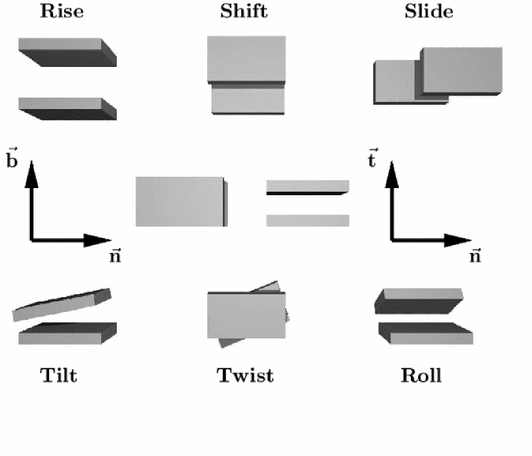
Figure 1: (Color online) Illustration of all six base-pair parameters and the corresponding coordinate system.

each step is characterized by four parameters: Ri, Sl, Sh, and Tw CalladineDrew99 . Within the given geometry a base pair can be characterized by its position $\mathbf{r}$ and the angle of its main axis with the $\mathbf{n}$/$\mathbf{b}$-axis ($\mathbf{n}$ points into the direction of the large axis, $\mathbf{b}$ points into the direction of the small axis, and $\mathbf{t}$, representing the tangent vector of the resulting helix, is perpendicular to the $\mathbf{n}$-$\mathbf{b}$- plane as it is illustrated in Fig. 1). At each step the center points are displaced by a distance $\sqrt{\mbox{Sl}^{2}+\mbox{Sh}^{2}}$ in the $\mathbf{n}-\mathbf{b}-$plane. The angle between successive steps is equal to the twist angle and the center points are located on a helix with radius $r=\sqrt{\mbox{Sl}^{2}+\mbox{Sh}^{2}}/(2\sin(\mbox{Tw}/2))$.

In the following we study the consequences of imposing a simple constraint on the bond lengths $l_{1}$ and $l_{2}$ representing the two sugar phosphate backbones (the rigid bonds connect the right and left edges of the bars along the $\mathbf{n}$-axis respectively). Ri is the typical height of a step which we will try to impose on the grounds that it represents the preferred stacking distance of neighboring base pairs. We choose $\mbox{Ri}=3.3\mbox{\AA}$ corresponding to the B-DNA value. One possibility to fulfill the constraint $l_{1}=l_{2}=l=6\mbox{\AA}$ is pure twist. In this case a relationship of the twist angle and the width of the base-pairs $d$, the backbone length $l$ and the imposed rise is obtained:

$$\mbox{Tw}=\arccos\left(\frac{d^{2}-2l^{2}+2\mbox{Ri}^{2}}{d^{2}}\right).$$ (1)

Another possibility is to keep the rotational orientation of the base pair ($\mbox{Tw}=0$), but to displace its center in the $\mathbf{n}$-$\mathbf{b}$-plane, in which case $\mbox{Ri}^{2}+\mbox{Sl}^{2}+\mbox{Sh}^{2}\equiv l^{2}$. With $\mbox{Sh}=0$, it results in a skewed ladder with skew angle $\arcsin(\mbox{Sl}/l)/\pi$ CalladineDrew99 .

The general case can be solved as well. In a first step a general condition is obtained that needs to be fulfilled by any combination of Sh, Sl, and Tw independently of Ri. For non-vanishing Tw this yields a relation between Sh and Sl:

$$\tan(\mbox{Tw})=\frac{\mbox{Sh}}{\mbox{Sl}}.$$ (2)

Using Eq. (2) the general equation can finally be solved:

$$\mbox{Sl}=\frac{1}{\sqrt{2}}\left[\cos(\frac{\mbox{Tw}}{2})^{2}\sqrt{\sec(\frac{\mbox{Tw}}{2})^{2}(2l^{2}-d^{2}-\mbox{Ri}^{2})}\,\right].$$ (3)

Eq. (3) is the result of the mechanical coupling of slide, shift and twist due to the backbones. Treating the rise again as a constraint the twist is reduced for increasing slide or shift motion.

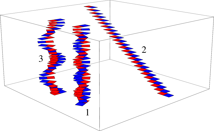
Figure 2: (Color online) Illustration of DNA geometry for a diameter of $d=16\mbox{\AA}$: (1) Twisted ladder with $\mbox{Sl}=\mbox{Sh}=0$, $\mbox{Ri}=3.3\mbox{\AA}$, $\mbox{Tw}\approx 2\pi/10$, (2) Skewed ladder with $\mbox{Tw}=\mbox{Sh}=0$, $\mbox{Ri}=3.4\mbox{\AA}$, $\mbox{Sl}\approx 5.0\mbox{\AA}$, (3) Helix with $\mbox{Tw}=2\pi/12$, $\mbox{Ri}=3.4\mbox{\AA}$, $\mbox{Sl}\approx 2.7\mbox{\AA}$, $\mbox{Sh}\approx 1.6\mbox{\AA}$.

The center-center distance $c$ of two neighboring base-pairs is given by

$$c=\sqrt{\mbox{Ri}^{2}+\mbox{Sl}^{2}\left(1+\tan(\mbox{Tw})^{2}\right)}.$$ (4)

For $\mbox{Tw}=0$ and a given value of Ri the center-center distance is equal to the backbone length $l$ and for $\mbox{Tw}=\arccos\left((d^{2}-2l^{2}+2\mbox{Ri}^{2})/d^{2}\right)$ one obtains $c=\mbox{Ri}$.

II.2 Thermal fluctuations

In this section we discuss how to calculate the effective coupling constants of a harmonic system valid within linear response theory describing the couplings of the base-pair parameters along the chain. Furthermore we show how to translate measured mean and mean squared values of the 6 microscopic base-pair parameters into macroscopic observables such as bending and torsional persistence length. This provides the linkage between the two descriptions: WLC (worm-like chain) versus SOP (stack-of-plates) model.

Within linear response theory it should be possible to map our model onto a Gaussian system where all translational and rotational degrees of freedom are harmonically coupled. We refer to this model as the stack-of-plates (SOP) model Hern_epjb_98 . The effective coupling constants are given by the second derivatives of the free energy in terms of base-pair variables around the equilibrium configuration. This yields $6\times 6$ matrices ${\cal K}^{nm}$ describing the couplings of the base-pair parameters of neighboring base-pairs along the chain:

$${\cal K}^{nm}=\frac{\partial^{2}{\cal F}}{\partial x^{n}_{i}\partial x^{m}_{j}}.$$ (5)

Therefore one can calculate the $(N-1)\times(N-1)$ correlation matrix ${\cal C}$ in terms of base-pair parameters. $N$ is thereby the number of base-pairs.

$$\langle{\cal C}\rangle=\begin{pmatrix}{\cal K}^{11}&{\cal K}^{12}&{\cal K}^{13}&{\cal K}^{14}&\ldots\\ {\cal K}^{12}&{\cal K}^{22}&{\cal K}^{23}&{\cal K}^{24}&\ldots\\ &&\ddots&&\end{pmatrix}^{-1}.$$ (6)

The inversion of ${\cal C}$ results in a generalized connectivity matrix with effective coupling constants as entries.

The following considerations are based on the assumption that one only deals with nearest-neighbor interactions. Then successive base-pair steps are independent of each other and the calculation of the orientational correlation matrix becomes feasible. In the absence of spontaneous displacements ($\mbox{Sl}=\mbox{Sh}=0$) and spontaneous bending angles ($\mbox{Ti}=\mbox{Ro}=0$) as it is the case for B-DNA going from one base-pair to the neighboring implies three operations. In order to be independent of the reference base pair one first rotates the respective base pair into the mid-frame with ${\cal{R}}(Tw_{sp}/2)$ (${\cal{R}}$ is a rotation matrix, $Tw_{sp}$ denotes the spontaneous twist), followed by a subsequent overall rotation in the mid-frame

$${\cal{A}}=\begin{pmatrix}{\mathbf{t_{i}}}\cdot{\mathbf{t_{i+1}}}&{\mathbf{t_{i}}}\cdot{\mathbf{b_{i+1}}}&{\mathbf{t_{i}}}\cdot{\mathbf{n_{i+1}}}\\ {\mathbf{b_{i}}}\cdot{\mathbf{t_{i+1}}}&{\mathbf{b_{i}}}\cdot{\mathbf{b_{i+1}}}&{\mathbf{b_{i}}}\cdot{\mathbf{n_{i+1}}}\\ {\mathbf{n_{i}}}\cdot{\mathbf{t_{i+1}}}&{\mathbf{n_{i}}}\cdot{\mathbf{b_{i+1}}}&{\mathbf{n_{i}}}\cdot{\mathbf{n_{i+1}}}\end{pmatrix}$$ (7)

taken into account the thermal motion of Ro, Ti and Tw, and a final rotation due to the spontaneous twist ${\cal{R}}(Tw_{sp}/2)$. The orientational correlation matrix between two neighboring base pairs can be written as $\langle{\cal{O}}_{i\,i+1}\rangle={\cal{R}}(Tw_{sp}/2)\,\langle{\cal{A}}\rangle\,{\cal{R}}(Tw_{sp}/2)$. ${\cal{A}}$ describes the fluctuations around the mean values. As a consequence of the independence of successive base-pair parameters one finds $\langle{\cal{O}}_{i\,j}\rangle=\left({\cal{R}}(Tw_{sp}/2)\,\langle{\cal{A}}\rangle\,{\cal{R}}(Tw_{sp}/2)\right)^{j-i}$ where the matrix product is carried out in the eigenvector basis of ${\cal{R}}(Tw_{sp}/2)\,\langle{\cal{A}}\rangle\,{\cal{R}}(Tw_{sp}/2)$. In the end one finds a relationship of the mean and mean squared local base-pair parameters and the bending and torsional persistence length. The calculation yields an exponentially decaying tangent-tangent correlation function $\langle\mathbf{t}(0)\cdot\mathbf{t}(s)\rangle=\exp(-s/l_{p})$ with a bending persistence length

$$l_{p}=\frac{2\langle\mbox{Ri}\rangle}{(\langle\mbox{Ti}^{2}\rangle+\langle\mbox{Ro}^{2}\rangle)}.$$ (8)

In the following we will calculate the torsional persistence length. Making use of a simple relationship between the local twist and the base-pair orientations turns out to be more convenient than the transfer matrix approach.

The (bi)normal-(bi)normal correlation function is an exponentially decaying function with an oscillating term depending on the helical repeat length $h=p\langle\mbox{Ri}\rangle$ and the helical pitch $p=2\pi/\langle\mbox{Tw}\rangle$ respectively, namely $\langle\mathbf{n}(0)\cdot\mathbf{n}(s)\rangle=\exp(-s/l_{n})\cos(2\pi\,s/h)$. The torsional persistence length $l_{n}=l_{b}$ can be calculated in the following way. It can be shown that the twist angle Tw of two successive base-pairs is related to the orientations $\{{\mathbf{t}},{\mathbf{b}},{\mathbf{n}}\}$ and $\{{\mathbf{t}^{\prime}},{\mathbf{b}^{\prime}},{\mathbf{n}^{\prime}}\}$ through

$$\cos(\mbox{Tw})=\frac{{\mathbf{n}}\cdot{\mathbf{n}^{\prime}}+{\mathbf{b}}\cdot{\mathbf{b}^{\prime}}}{1+{\mathbf{t}}\cdot{\mathbf{t}^{\prime}}}.$$ (9)

Taking the mean and using the fact that the orientational correlation functions and twist correlation function decay exponentially

$$\exp(-1/l_{Tw})=\frac{2\exp(-1/l_{n})}{1+\exp(-1/l_{p})}$$ (10)

yields in the case of stiff filaments a simple expression of $l_{n}$ depending on $l_{p}$ and $l_{Tw}$:

$$\frac{l_{n}}{2}=\frac{l_{b}}{2}=\left(\frac{2}{l_{Tw}}+\frac{1}{l_{p}}\right)^{-1},$$ (11)

where the twist persistence length is defined as

$$l_{Tw}=\frac{\langle\mbox{Ri}\rangle}{\langle\mbox{Tw}^{2}\rangle}.$$ (12)

III Model and methods

Qualitatively the geometrical considerations suggest a B-DNA like ground state and the transition to a skewed ladder conformation under the influence of a sufficiently high stretching force, because this provides the possibility to lengthen the chain and to partially conserve stacking. Quantitative modeling requires the specification of a Hamiltonian.

III.1 Introduction of the Hamiltonian

The observed conformation of a dinucleotide base-pair step represents a compromise between (i) the base stacking interactions (bases are hydrophobic and the base-pairs can exclude water by closing the gap in between them) and (ii) the preferred backbone conformation (the equilibrium backbone length restricts the conformational space accessible to the base-pairs) PackerHunter_jmb_98 . Packer and Hunter PackerHunter_jmb_98 have shown that roll, tilt and rise are backbone-independent parameters. They depend mainly on the stacking interaction of successive base-pairs. In contrast twist is solely controlled by the constraints imposed by a rigid backbone. Slide and shift are sequence-dependent. While it is possible to introduce sequence dependant effects into our model, they are ignored in the present paper.

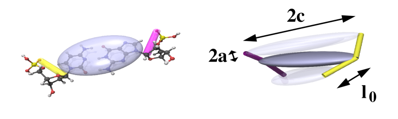
Figure 3: (Color online) (left) Illustration of the underlying idea. The base-pairs are represented as rigid ellipsoids. The sugar-phosphate backbone is treated as semi-rigid springs connecting the edges of the ellipsoid. (right) Introduced interactions lead to a right-handed twisted structure.

In the present paper we propose a generic model for DNA where the molecule is described as a stack of thin, rigid ellipsoids representing the base pairs (Fig. 3). The shape of the ellipsoids is given by three radii $a$, $b$, $c$ of the main axes in the body frames which can be used to define a structure matrix

$${\cal{S}}=\begin{pmatrix}a&0&0\\ 0&b&0\\ 0&0&c\end{pmatrix}$$ (13)

$2a$ corresponds to the thickness, $2b$ to the depth which is a free parameter in the model, and $2c=18\mbox{\AA}$ to the width of the ellipsoid which is fixed to the diameter of a B-DNA helix. The thickness $2a$ will be chosen in such a way that the minimum center-center distance for perfect stacking reproduces the experimentally known value of $3.3\mbox{\AA}$.

The attraction and the excluded volume between the base pairs is modeled by a variant of the Gay-Berne potential ralf_GB ; Gay-Berne for ellipsoids of arbitrary shape ${\cal S}_{i}$, relative position ${\vec{r}}_{12}$ and orientation ${\bf A}_{i}$. The potential can be written as a product of three terms:

$$U({\bf A}_{1},{\bf A}_{2},{\vec{r}}_{12}) =U_{\mathrm{r}}({\bf A}_{1},{\bf A}_{2},{\vec{r}}_{12})$$

$$\times\eta_{12}({\bf A}_{1},{\bf A}_{2},{\hat{r}}_{12})\,\chi_{12}({\bf A}_{1},{\bf A}_{2},{\hat{r}}_{12}).$$ (14)

The first term controls the distance dependence of the interaction and has the form of a simple LJ potential

$$U_{\mathrm{r}}=4\epsilon_{\mathrm{G}B}\left(\left(\frac{\sigma}{h+\gamma\sigma}\right)^{12}-\left(\frac{\sigma}{h+\gamma\sigma}\right)^{6}\right)$$ (15)

where the interparticle distance $r$ is replaced by the distance $h$ of closest approach between the two bodies:

$$h\equiv\min(|\vec{r}_{i}-\vec{r}_{j}|)\ \forall(i,j)$$ (16)

with $i\in{\mathrm{B}ody\,1}$ and $j\in{\mathrm{B}ody\,2}$. The range of interaction is controlled by an atomistic length scale $\sigma=3.3\mbox{\AA}$, representing the effective diameter of a base-pair.

In general, the calculation of $h$ is non-trivial. We use the following approximative calculation scheme which is usually employed in connection with the Gay-Berne potential:

$$h({\bf A}_{1},{\bf A}_{2},{\vec{r}}_{12}) = r_{12}-\sigma_{12}({\bf A}_{1},{\bf A}_{2},\hat{r}_{12})$$ (17)

$$\sigma_{12}({\bf A}_{1},{\bf A}_{2},\hat{r}_{12}) = [{\frac{1}{2}}\hat{r}_{12}^{T}{\bf G}_{12}^{-1}({\bf A}_{1},{\bf A}_{2})\hat{r}_{12}]^{-1/2}$$ (18)

$${\bf G}_{12}({\bf A}_{1},{\bf A}_{2}) = {\bf A}_{1}^{T}{\bf S}_{1}^{2}{\bf A}_{1}+{\bf A}_{2}^{T}{\bf S}_{2}^{2}{\bf A}_{2}.$$ (19)

In the present case of oblate objects with rather perfect stacking behavior Eq. (17) produces only small deviations from the exact solution of Eq. (16).

The other two terms in Eq. (III.1) control the interaction strength as a function of the relative orientation ${\bf A}_{1}^{t}{\bf A}_{2}$ and position $\vec{r}_{12}$ of interacting ellipsoids:

$$\eta_{12}({\bf A}_{1},{\bf A}_{2},{\hat{r}}_{12}) = \frac{\det[{\bf S}_{1}]/\sigma_{1}^{2}+\det[{\bf S}_{2}]/\sigma_{2}^{2}}{\left(\det[{\bf H}_{12}]/(\sigma_{1}+\sigma_{2})\right)^{1/2}}$$ (20)

$${\bf H}_{12}({\bf A}_{1},{\bf A}_{2},\hat{r}_{12}) = \frac{1}{\sigma_{1}}{\bf A}_{1}^{T}{\bf S}_{1}^{2}{\bf A}_{1}+\frac{1}{\sigma_{2}}{\bf A}_{2}^{T}{\bf S}_{2}^{2}{\bf A}_{2}$$ (21)

$$\sigma_{i}({\bf A}_{i},\hat{r}_{12}) \equiv \left(\hat{r}_{12}^{T}\ \ {\bf A}_{1}^{T}{\bf S}_{i}^{-2}{\bf A}_{1}\ \ \hat{r}_{12}\right)^{-1/2}$$ (22)

and

$$\chi_{12}({\bf A}_{1},{\bf A}_{2},\hat{r}_{12}) = [2\hat{r}_{12}^{T}\ \ {\bf B}_{12}^{-1}({\bf A}_{1},{\bf A}_{2})\ \hat{r}_{12}]$$ (23)

$${\bf B}_{12}({\bf A}_{1},{\bf A}_{2}) = {\bf A}_{1}^{T}{\bf E}_{1}{\bf A}_{1}+{\bf A}_{2}^{T}{\bf E}_{2}{\bf A}_{2}$$ (24)

with

$${\bf E}_{i}=\sigma\begin{pmatrix}\frac{a_{i}}{b_{i}\,c_{i}}&0&0\\ 0&\frac{b_{i}}{a_{i}\,c_{i}}&0\\ 0&0&\frac{c_{i}}{a_{i}\,b_{i}}\end{pmatrix}=\frac{\sigma}{\det[{\bf S}_{i}]}{\bf S}_{i}^{2}.$$ (25)

We neglect electrostatic interactions between neighboring base-pairs since at physiological conditions the stacking interaction dominates Hunter_jmb_92 ; CalladineDrew99 .

At this point we have to find appropriate values for the thickness $2a$ and the parameter $\gamma$ of Eq. (15). Both parameters influence the minimum of the Gay-Berne potential. There are essentially two possible procedures. One way is to make use of the parameterization result of Everaers and Ejtehadi ralf_GB , i.e. $\gamma=2^{1/6}-30^{-1/6}$, and to choose a value of $a\approx 0.7$ that yields the minimum center-center distance of $3.3\mbox{\AA}$ for perfect stacking. Unfortunately it turns out that the fluctuations of the bending angles strongly depend on the flatness of the ellipsoids. The more flat the ellipsoids are the smaller are the fluctuations of the bending angles so that one ends up with extremely stiff filaments with a persistence length of a few thousand base-pairs. This can be seen clearly for the extreme case of two perfectly stacked plates: each bending move leads then to an immediate overlap of the plates. That is why we choose the second possibility. We keep $\gamma$ as a free parameter that is used in the end to shift the potential minimum to the desired value and fix the width of the ellipsoids to be approximately half the known rise value $a=1.55\mbox{\AA}$. This requires $\gamma=1.07$.

The sugar phosphate backbone is known to be nearly inextensible. The distance between adjacent sugars varies from $5.5\mbox{\AA}$ to $6.5\mbox{\AA}$ CalladineDrew99 . This is taken into account by two stiff springs with length $l_{1}=l_{2}=6.0\mbox{\AA}$ connecting neighboring ellipsoids (see Fig. 3). The anchor points are situated along the centerline in $\vec{n}$-direction (compare Fig. 1 and Fig. 3) with a distance of $\pm 8\mbox{\AA}$ from the center of mass. The backbone is thus represented by an elastic spring with non-zero spring length $l_{0}=6\mbox{\AA}$

$${\cal H}_{el}=\frac{k}{2}\left[(|\mathbf{r}_{1,i+1}-\mathbf{r}_{1,i}|-l_{0})^{2}+(|\mathbf{r}_{2,i+1}-\mathbf{r}_{2,i}|-l_{0})^{2}\right].$$ (26)

Certainly a situation where the backbones are brought closer to one side of the ellipsoid so as to create a minor and major groove would be a better description of the B-DNA structure. But it turns out that due to the ellipsoidal shape of the base-pairs and due to the fact that the internal base-pair degrees of freedom (propeller twist, etc.) cannot relax a non-B-DNA-like ground state is obtained where roll and slide motion is involved.

The competition between the GB potential that forces the ellipsoids to maximize the contact area and the harmonic springs with non-zero spring length that does not like to be compressed leads to a twist in either direction of the order of $\pm\pi/5$. The right-handedness of the DNA helix is due to excluded volume interactions between the bases and the backbone CalladineDrew99 which we do not represent explicitly. Rather we break the symmetry by rejecting moves which lead to local twist smaller than $-\pi/18$.

Thus we are left with three free parameters in our model, the GB energy depth $\epsilon=\min(U)$ which controls the stacking interaction, the spring constant $k$ which controls the torsional rigidity, and the depth $b$ of the ellipsoids which influences mainly the fluctuations of the bending angles. All other parameters such as the width and the height of the ellipsoids, or the range of interaction $\sigma=3.3\mbox{\AA}$ which determines the width of the GB potential are fixed so as to reproduce the experimental values for B-DNA.

III.2 MC simulation

In our model all interactions are local and it can therefore conveniently be studied using a MC scheme. In addition to trial moves consisting of local displacements and rotations of one ellipsoid by a small amplitude, it is possible to employ global moves which modify the position and the orientation of large parts of the chain. The moves are analogous of (i) the well-known pivot move Binder_00 , and (ii) a crankshaft move where two randomly chosen points along the chain define the axis of rotation around which the inner part of the chain is rotated. The moves are accepted or rejected according to the Metropolis scheme Metropolis_jcp_53 .

Fig. 4 shows that these global moves significantly improve the efficiency of the simulation. We measured the correlation time $\tau$ of the scalar product of the tangent vectors of the first and the last monomer of 200 independent simulation runs with $N=10,\,20,\,50$ monomers using (i) only local moves and (ii) local and global moves (ratio 1:1). The correlation time of the global moves is independent of the chain length with $\tau_{global}\approx 78\,\mbox{ sweeps}$ whereas $\tau_{local}$ scales as $N^{3}$.

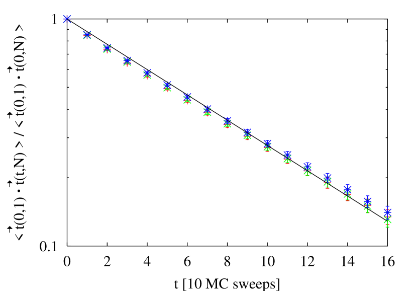
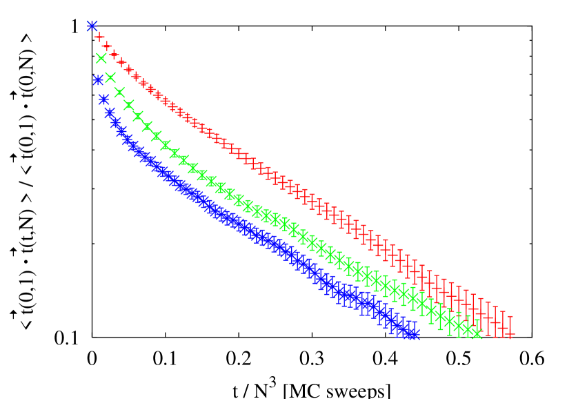
Figure 4: (Color online) Time correlation functions of the scalar product of the tangent vectors of the first and the last monomer $\tau=\vec{t}(0,1)\cdot\vec{t}(t,N)$ with $N=10\mbox{ (red)},\,N=20\mbox{ (green)},\,N=50\mbox{ (blue)}$ for (a) global and (b) local moves. It is observed that $\tau_{global}$ is independent of the chain length $N$ whereas $\tau_{local}$ scales as $N^{3}$. The ’time’ is measured in units of sweeps where one MC sweep corresponds to $N$ trials. The CPU time for one sweep scales as $N^{2}$ in case of global moves and as $N$ in case of local moves. Thus the simulation time $t$ scales as $t_{local}\propto N^{4}$ and $t_{global}\propto N^{2}$.

Each simulation run comprises $10^{6}$ MC sweeps where one MC sweep corresponds to $2N$ trials (one rotational and one translational move per base pair) with $N$ denoting the number of monomers. The amplitude is chosen such that the acceptance rate equals approximately to $50$%. Every 1000 sweeps we store a snapshot of the DNA conformation. We measured the ’time’ correlation functions of the end-to-end distance, the rise of one base-pair inside the chain and all three orientational angles of the first and the last monomer and of two neighboring monomers inside the chain in order to extract the longest relaxation time $\tau_{max}$. We observe $\tau_{max}<1000$ for all simulation runs.

An estimate for the CPU time required for one sweep for chains of length $N=100$ on a AMD Athlon MP 2000+ processor results in $0.026s$ which is equivalent to $1.33\,10^{-4}s$ per move.

III.3 Energy minimization

We complemented the simulation study by zero temperature considerations that help to discuss the geometric structure that is obtained by the introduced interactions and to rationalize the MC simulation data. Furthermore they can be used to obtain an estimate of the critical force $f_{crit}$ that must be applied to enable the structural transition from B-DNA to the overstretched S-DNA configuration as a function of the model parameters $\{\epsilon,k,b\}$.

IV Results

In the following we will try to motivate an appropriate parameter set $\{\epsilon,\,k,\,b\}$ that can be used for further investigations within the framework of the presented model. Therefore we explore the parameter dependence of experimental observables such as the bending persistence length of B-DNA $l_{p}\approx 150\mbox{bp}$, the torsional persistence length $l_{t}\approx 260\mbox{bp}$ Strick_genetica_99 , the mean values and correlations of all six base-pair parameters and the critical pulling force $f_{crit}\approx 65\mbox{pN}$ Cluzel_sci_96 ; Lavery_genetica_99 ; Lavery_jpcm_02 ; Smith_cosb_00 that must be applied to enable the structural transition from B-DNA to the overstretched S-DNA configuration. In fact, static and dynamic contributions to the bending persistence length $l_{p}$ of DNA are still under discussion. It is known that $l_{p}$ depends on both the intrinsic curvature of the double helix due to spontaneous bending of particular base-pair sequences and the thermal fluctuations of the bending angles. Bensimon et al. Bensimon_epl_98 introduced disorder into the WLC model by an additional set of preferred random orientation between successive segments and found the following relationship between the pure persistence length $l_{pure}$, i.e. without disorder, the effective persistence length $l_{eff}$ and the persistence length $l_{disorder}$ caused by disorder:

$$\frac{l_{eff}}{l_{pure}}=\begin{cases}1-\frac{\sqrt{\frac{l_{pure}}{l_{disorder}}}}{2}&\frac{l_{pure}}{l_{disorder}}\ll 1\\ \frac{2}{\frac{l_{pure}}{l_{disorder}}}&\frac{l_{pure}}{l_{disorder}}\gg 1\end{cases}.$$ (27)

Since we are dealing with intrinsically straight filaments with $1/l_{disorder}=0$, we measure $l_{pure}$. Recent estimates of $l_{disorder}$ range between $430$ Bednar_jmb_95 and $4800$ Vologodskaia_jmb_02 base-pairs using cryo-electron microscopy and cyclization experiments respectively implicating values between $105$ and $140$ base-pairs for $l_{pure}$.

IV.1 Equilibrium structure

As a first step we study the equilibrium structure of our chains as a function of the model parameters. To investigate the ground state conformation we rationalize the MC simulation results with the help of the geometrical considerations and minimum energy calculations. In the end we will choose parameters for which our model reproduces the experimental values of B-DNA  CalladineDrew99 :

$$\langle\mbox{Ri}\rangle = 3.3-3.4\mbox{\AA}$$

$$\langle\mbox{Sl}\rangle = 0\mbox{\AA}$$

$$\langle\mbox{Sh}\rangle = 0\mbox{\AA}$$

$$\langle\mbox{Tw}\rangle = 2\pi/10.5-2\pi/10$$

$$\langle\mbox{Ti}\rangle = 0$$

$$\langle\mbox{Ro}\rangle = 0.$$

We use the following reduced units in our calculations. The energy is measured in units of $k_{B}T$, lengths in units of Å, forces in units of $k_{B}T\mbox{{\AA}}^{-1}\approx 40\mbox{pN}$.

$\,T\,$	$\langle\mbox{Ri}\rangle$	$\langle\mbox{Sh}\rangle$	$\langle\mbox{Sl}\rangle$	$\langle\mbox{Tw}\rangle$	$\langle\mbox{Ti}\rangle$	$\langle\mbox{Ro}\rangle$	$\langle c\rangle$	$l_{p}$
0	3.26	0.0	0.0	0.64	0.0	0.0	3.26	$\infty$
1	3.37	0.01	-0.01	0.62	0.0	0.0	3.47	172.8
2	3.76	-0.01	-0.03	0.47	0.0	0.0	4.41	25.3
3	4.10	-0.01	0.01	0.34	0.0	-0.01	5.07	14.4
5	4.30	0.03	-0.02	0.27	0.0	0.01	5.39	13.6

Table 1: Dependence of mean values of all six step parameters and of the mean center-center distance $\langle c\rangle$ on the temperature for $2b=11\mbox{\AA}$, $\epsilon=20k_{B}T$, $k=64k_{B}T/\mbox{\AA}^{2}$. $\langle\mbox{Ri}\rangle$, $\langle\mbox{Sh}\rangle$, $\langle\mbox{Sl}\rangle$ and $\langle c\rangle$ are measured in [$\AA$], $l_{p}$ in base-pairs.

We start by minimizing the energy for the various conformations shown in Fig. 2 to verify that our model Hamiltonian indeed prefers the B-Form. Since we have only local (nearest neighbor) interactions we can restrict the calculations to two base pairs. There are three local minima which have to be considered: (i) a stacked, twisted conformation with $\mbox{Ri}=3.3,\,\mbox{Sl,\,Sh,\,Ti,\,Ro}=0,\,\mbox{Tw}=\pi/10$, (ii) a skewed ladder with $\mbox{Ri}=3.3,\,\mbox{Sl}=5.0,\,\mbox{Sh,\,Tw,\,Ti,\,Ro}=0$, and (iii) an unwound helix with $\mbox{Ri}=6.0,\,\mbox{Sl,\,Sh,\,Ti,\,Ro}=0,\,\mbox{Tw}=0$. Without an external pulling force the global minimum is found to be the stacked twisted conformation.

We investigated the dependence of Ri and Tw on the GB energy depth $\epsilon$ that controls the stacking energy for different spring constants $k$. Ri depends neither on $\epsilon$ nor on $k$ nor on $b$. It shows a constant value of $\mbox{Ri}\approx 3.3\mbox{\AA}$ for all parameter sets $\{\epsilon,k,b\}$. The resulting Tw of the minimum energy calculation coincides with the geometrically determined value under the assumption of fixed Ri up to a critical $\epsilon$. Up to that value the springs behave effectively as rigid rods. The critical $\epsilon$ is determined by the torque $\tau(k,\epsilon)$ that has to be applied to open the twisted structure for a given value of Ri.

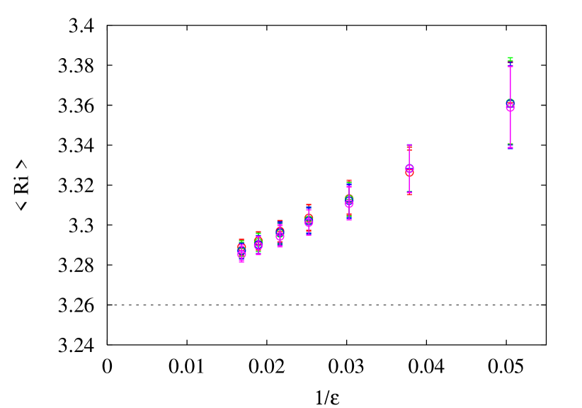
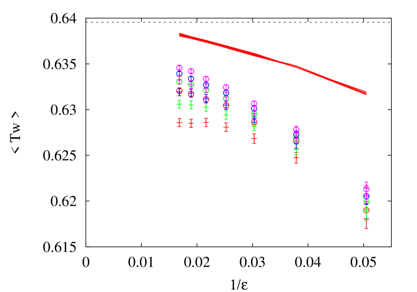
Figure 5: (Color online) (a) Rise [Å] and (b) twist as a function of $\epsilon$ [$k_{B}T$] for $2b=8,\,9,\,10,\,11\mbox{\AA}$ (red, green, blue, purple). For every $b$ there are two data sets for $k=32\mbox{ (plus)},\,64\mbox{ (circles)}$ [$k_{B}T/\mbox{\AA}^{2}$]. The dotted line corresponds to the minimum energy value. $\langle\mbox{Ri}\rangle$ depends only on $\epsilon$. In the limit of $\epsilon\rightarrow\infty$ the minimum energy value is reached.
(b) In addition to the MC data and the minimum energy calculation we calculated the twist with Eq. (1) using the measured mean rise values of (a). One can observe that $\langle\mbox{Tw}\rangle$ changes with all three model parameters. Increasing $y$ and $k$ decreases especially the fluctuations of Tw and Sh so that $\langle\mbox{Tw}\rangle$ increases as a result of the mechanical coupling of the shift and twist motion. In the limit of $\epsilon,k\rightarrow\infty$ the minimum energy value is reached.

Using MC simulations we can study the effects arising from thermal fluctuations. Plotting $\langle\mbox{Ri}\rangle$, and $\langle\mbox{Tw}\rangle$ as a function of the GB energy depth $\epsilon$ one recognizes that in general $\langle\mbox{Ri}\rangle$ is larger than $\mbox{Ri}(T=0)$. It converges only for large values of $\epsilon$ to the minimum energy values. This can be understood as follows. Without fluctuations the two base pairs are perfectly stacked taking the minimum energy configuration $\mbox{Ri}=3.3\mbox{\AA}$, $\mbox{Sl,\,Sh,\,Ti,\,Ro}=0$, and $\mbox{Tw}=\pi/10$. As the temperature is increased the fluctuations can only occur to larger Ri values due to the repulsion of neighboring base pairs. A decrease of Ri would cause the base-pairs to intersect. Increasing the stacking energy reduces the fluctuations in the direction of the tangent vector and leads to smaller $\langle\mbox{Ri}\rangle$ value. In the limit $\epsilon\rightarrow\infty$ it should reach the minimum energy value which is observed from the simulation data. In turn the increase of the mean value of rise results in a smaller twist angle $\langle\mbox{Tw}\rangle$. We can calculate with the help of Eq. (1) the expected twist using the measured mean values of $\langle\mbox{Ri}\rangle$. Fig. 5 shows that there is no agreement.

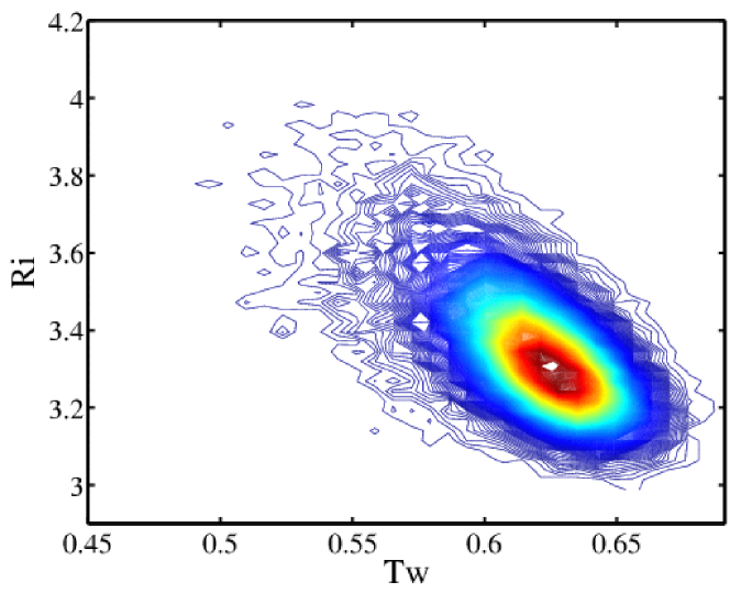
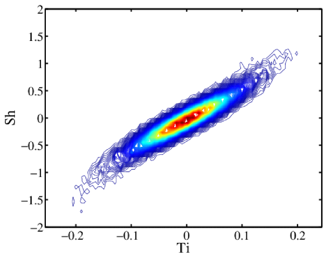
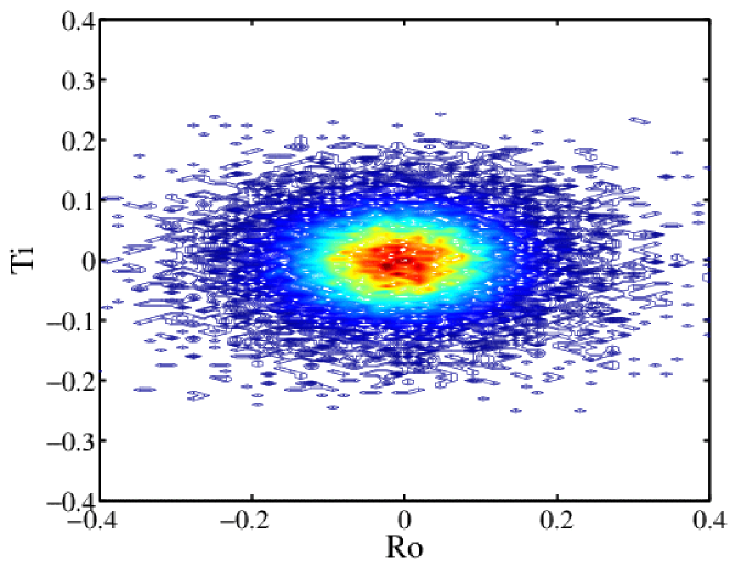
Figure 6: (Color online) Contour plots of measured clouds for rise-twist, shift-tilt, and roll-tilt to demonstrate internal couplings and the anisotropy of the bending angles ($2b=11\mbox{\AA}$, $\epsilon=20k_{B}T$, $k=64k_{B}T/\mbox{\AA}^{2}$).

The deviations are due to fluctuations in Sl and Sh which cause the base-pairs to untwist. This is the mechanical coupling of Sl, Sh, and Tw due to the backbones already mentioned in section II.1. It is observed that a stiffer spring $k$ and a larger depth of the ellipsoids $b$ result in larger mean twist values. Increasing the spring constant $k$ means decreasing the fluctuations of the twist and, due to the mechanical coupling, of the shift motion around the mean values which explains the larger mean twist values. An increase of the ellipsoidal depth $b$ in turn decreases the fluctuations of the bending angles. The coupling of the tilt fluctuations with the shift fluctuations leads to larger values for $\langle\mbox{Tw}\rangle$. The corresponding limit where $\langle\mbox{Tw}\rangle\rightarrow\mbox{Tw}(\mbox{T}=0)$ is given by $k,\epsilon\rightarrow\infty$.

The measurement of the mean values of all six base-pair step parameters for different temperatures is shown in Table 1. One can see that with increasing temperature the twist angles decrease while the mean value of rise increase. The increase of the center-center distance is not only due to fluctuations in Ri but also due to fluctuations in Sl and Sh. That is why there are strong deviations of $\langle c\rangle$ from $\langle\mbox{Ri}\rangle$ even though the mean values of Sl and Sh vanish. Note that the mean backbone length $\langle l\rangle$ always amounts to about $6\mbox{\AA}$.

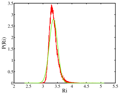
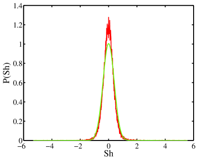
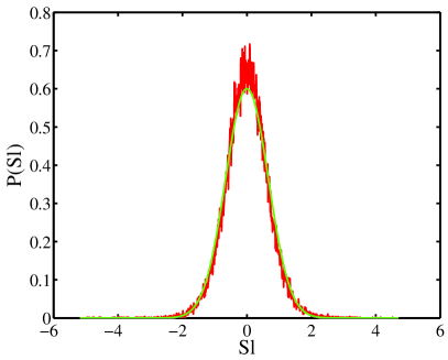
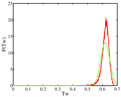
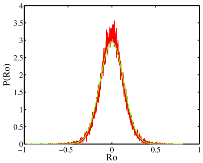
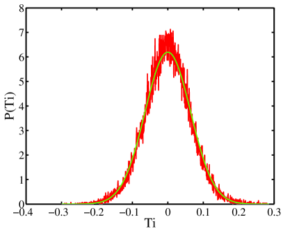
Figure 7: (Color online) Comparison of probability distribution functions of all base-pair parameters for $\epsilon=20k_{B}T$, $k=64k_{B}T/\mbox{\AA}^{2}$, $2b=8\mbox{\AA}$. The Gaussians are plotted with the measured mean and mean squared values of the MC simulation.

The calculation of the probability distribution functions of all six base-pair parameters shows that especially the rise and twist motion do not follow a Gaussian behavior. The deviation of the distribution functions from the Gaussian shape depends mainly on the stacking energy determined by $\epsilon$. For smaller values of $\epsilon$ one observes larger deviations than for large $\epsilon$ values.

It is worthwhile to mention that there are mainly two correlations between the base-pair parameters. The first is a microscopic twist-stretch coupling determined by a correlation of Ri and Tw, i.e. an untwisting of the helix implicates larger rise values. A twist-stretch coupling was introduced in earlier rod models Kamien_epl_97 ; Marko_epl_97 ; Nelson_bpj_98 motivated by experiments with torsionally constrained DNA Strick_sci_96 which allow for the determination of this constant. Here it is the result of the preferred stacking of neighboring base-pairs and the rigid backbones. The second correlation is due to constrained tilt motion. If we return to our geometrical ladder model we recognize immediately that a tilt motion alone will always violate the constraint of fixed backbone length $l$. Even though we allow for backbone fluctuations in the simulation the bonds are very rigid which makes tilting energetically unfavorable. To circumvent this constraint tilting always involves a directed shift motion.

Fig. 6 shows that we recover the anisotropy of the bending angles Ro and Ti as a result of the spatial dimensions of the ellipsoids. Since the overlap of successive ellipsoids is larger in case of rolling it is more favorable to roll than to tilt.

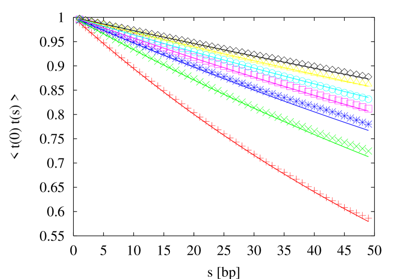
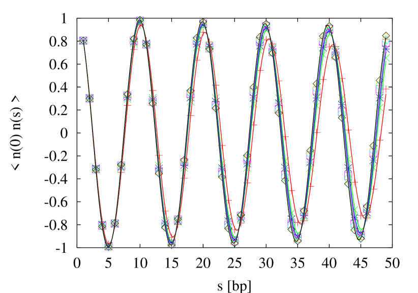
Figure 8: (Color online) Comparison of analytical expressions Eqs. (8) and (11) for $l_{p}$ and $l_{n}$ (solid lines) with numerically calculated orientational correlation functions (data points) for $2b=8\mbox{\AA}$, $k=64k_{B}T/\mbox{\AA}^{2}$, and $\epsilon=20,\,\ldots,\,60$ [$k_{B}T$] (from bottom to top).

The correlations can be quantified by calculating the correlation matrix ${\cal C}$ of Eq. (6). Inverting ${\cal C}$ yields the effective coupling constants of the SOP model ${\cal K}={\cal C}^{-1}$. Due to the local interactions it suffices to calculate mean and mean squared values of Ri, Sl, Sh, Tw, Ro, and Ti characterizing the ’internal’ couplings of the base-pairs:

$${\cal C}=(\sigma)_{ij},\,\forall i,j\in\{1,\ldots,6\}$$ (28)

with $\sigma_{x,y}=\langle xy\rangle-\langle x\rangle\langle y\rangle$.

IV.2 Bending and torsional rigidity

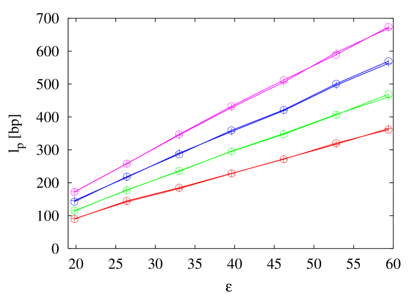
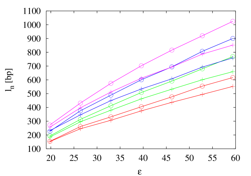
Figure 9: (Color online) Dependency of (a) bending persistence length $l_{p}$ and (b) torsional persistence length $l_{n}$ on the spring constant $k$, the width of the ellipsoids $b$ and the energy depth $\epsilon$. We measured the persistence lengths for varying width sizes $2b=8,\,9,\,10,\,11\mbox{\AA}$ (red, green, blue, purple) and for two different spring constants $k=32\mbox{ (plus)},\,64\mbox{ (circles)}$ [$k_{B}T/\mbox{\AA}^{2}$]. The bending persistence length depends solely on $b$ and $\epsilon$. It gets larger for larger $\epsilon$ and $b$ values. But it does not depend on $k$ (the curves for different $k$ values corresponding to the same width $b$ lie one upon the other). The torsional persistence length in turn depends on $k$, since a change of twist for constant Ri is proportional to a change in bond length.

The correlation matrix of Eq. (28) can also be used to check eqs. (8) and (11). Therefore we measured the orientational correlation functions $\langle\mathbf{t}_{i}\cdot\mathbf{t}_{j}\rangle$, $\langle\mathbf{n}_{i}\cdot\mathbf{n}_{j}\rangle$, $\langle\mathbf{b}_{i}\cdot\mathbf{b}_{j}\rangle$ and compared the results to the analytical expressions as it is illustrated in Fig. 8. The agreement is excellent.

The simulation data show that the bending persistence length does not depend on the spring constant $k$. But it strongly depends on $\epsilon$ being responsible for the energy that must be paid to tilt or roll two respective base pairs. Since a change of twist for constant Ri is proportional to a change in bond length the bond energy contributes to the twist persistence length explaining the dependence of $l_{Tw}$ on $k$ (compare Fig. 9).

We also measured the mean-square end-to-end distance $\langle R_{E}^{2}\rangle$ and find that $\langle R_{E}^{2}\rangle$ deviates from the usual WLC chain result due to the compressibility of the chain. So as to investigate the origin of the compressibility we calculate $\langle R_{E}^{2}\rangle$ for the following geometry. We consider two base-pairs without spontaneous bending angles such that the end-to-end vector $\vec{R}_{E}$ can be expressed as

$$\vec{R}_{E}=\sum_{i}\vec{c}_{i}=\sum_{i}(\mbox{Ri}\,{\mathbf{t}}_{i}+\mbox{Sh}\,{\mathbf{b}}_{i}+\mbox{Sl}\,{\mathbf{n}}_{i}).$$ (29)

The coordinate system $\{{\mathbf{t}}_{i},{\mathbf{b}}_{i},{\mathbf{n}}_{i}\}$ is illustrated in Fig. 1. $\vec{c}_{i}$ denotes the center-center distance of two neighboring base-pairs. Since successive base-pair step parameters are independent of each other, and Ri and Sh and Sl are uncorrelated the mean-square end-to-end distance $\langle R_{E}^{2}\rangle$ is given by

$$\begin{split}\langle R_{E}^{2}\rangle&=\sum_{i}(\langle c_{i}^{2}\rangle-\langle\mbox{Ri}\rangle^{2})+\sum_{i}\sum_{j}\langle\mbox{Ri}\rangle^{2}\langle{\mathbf{t}}_{i}\cdot{\mathbf{t}}_{j}\rangle\\ &=\frac{N\langle\mbox{Ri}\rangle}{\gamma}+2N\langle\mbox{Ri}\rangle l_{p}-2l_{p}^{2}\left(1-\exp\left(-\frac{N\langle\mbox{Ri}\rangle}{l_{p}}\right)\right).\end{split}$$ (30)

$N$ denotes the number of base-pairs. Note that $\langle\mbox{Sl}\rangle$ and $\langle\mbox{Sh}\rangle$ vanish. Using $\langle c_{i}^{2}\rangle=\langle\mbox{Ri}^{2}\rangle+\langle\mbox{Sh}^{2}\rangle+\langle\mbox{Sl}^{2}\rangle$ the stretching modulus $\gamma$ is simply given by

$$\gamma=\frac{\langle\mbox{Ri}\rangle}{(\langle\mbox{Ri}^{2}\rangle-\langle\mbox{Ri}\rangle^{2})+\langle\mbox{Sh}^{2}\rangle+\langle\mbox{Sl}^{2}\rangle}.$$ (31)

We compared the data for different temperatures $T$ to Eq. (30) using the measured bending persistence lengths $l_{p}$ and stretching moduli $\gamma$ (see Fig. 10). The agreement is excellent.

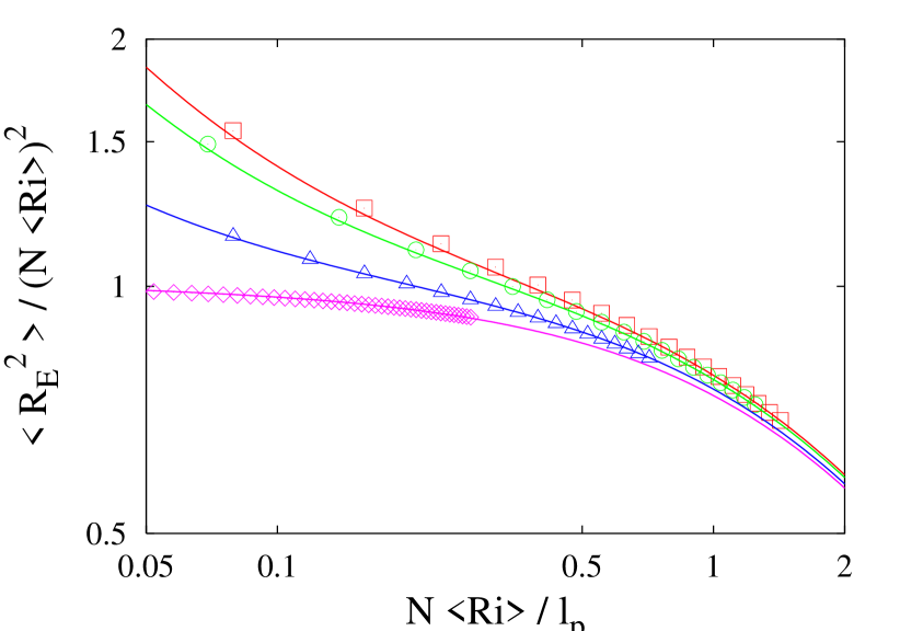
Figure 10: (Color online) Comparison of the simulation data with $\epsilon=20k_{B}T$, $k=64k_{B}T/\mbox{\AA}^{2}$, $2b=11\mbox{\AA}$, and $T=1,2,3,5$ (from top to bottom) to Eqs. (8), (30) and (31) (solid lines). Using the measured bending persistence lengths and the stretching moduli we find a good agreement with the predicted behavior. For $T=1$ we obtain $\gamma=6.02\mbox{\AA}^{-1}$.

This indicates that transverse slide and shift fluctuations contribute to the longitudinal stretching modulus of the chain.

IV.3 Stretching

Extension experiments on double-stranded B-DNA have shown that the overstretching transition occurs when the molecule is subjected to stretching forces of $65\mbox{pN}$ or more Smith_cosb_00 . The DNA molecule thereby increases in length by a factor of $1.8$ times the normal contour length. This overstretched DNA conformation is called S-DNA. The structure of S-DNA is still under discussion. First evidence of possible S-DNA conformations were provided by Lavery et al. Cluzel_sci_96 ; Lavery_genetica_99 ; Lavery_jpcm_02 using atomistic computer simulations.

In principle one can imagine two possible scenarios how the transition from B-DNA to S-DNA occurs within our model. Either the chain untwists and unstacks resulting in an untwisted ladder with approximately $1.8$ times the equilibrium length, or the chain untwists and the base-pairs slide against each other resulting in a skewed ladder with the same S-DNA length. The second scenario should be energetically favorable since it provides a possibility to partially conserve the stacking of successive base-pairs. In fact molecular modeling of the DNA stretching process Cluzel_sci_96 ; Lavery_genetica_99 ; Lavery_jpcm_02 yielded both a conformation with strong inclination of base-pairs and an unwound ribbon depending on which strand one pulls.

We expect that the critical force $f_{crit}$ where the structural transition from B-DNA to overstretched S-DNA occurs depends only on the GB energy depth $\epsilon$ controlling the stacking energy. So as a first step to find an appropriate value of $\epsilon$ as input parameter for the MC simulation we minimize the Hamiltonian with an additional stretching energy $E_{pull}=fc_{i,i+1}$, where the stretching force acts along the center-of-mass axis, with respect to Ri, Sl and Tw for a given pulling force $f$.

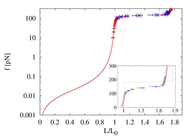
Figure 11: (Color online) Force-extension relation calculated by minimum energy calculation (black) and obtained by MC simulation (red) for $50$ (red) and $500$ (blue) base-pairs. The red solid line represents the analytical result of the WLC. (inset) The deviation between energy minimization (black dotted line) and MC in the critical force is due to entropic contributions.

Fig. 11 shows the resulting stress-strain curve. First the pulling force acts solely against the stacking energy up to the critical force where a jump from $L(f_{crit-})/L_{0}\approx 1.05$ to $L(f_{crit+})/L_{0}=\sqrt{\mbox{Ri}^{2}+\mbox{Sl}^{2}}/\mbox{Ri}\approx 1.8$ occurs, followed by another slow increase of the length caused by overstretching the bonds. $L_{0}=L(F=0)=\mbox{Ri}$ denotes the stress-free center-of-mass distance. As already mentioned three local minima are obtained: (i) a stacked, twisted conformation, (ii) a skewed ladder, and (iii) an unwound helix. The strength of the applied stretching force determines which of the local minima becomes the global one. The global minimum for small stretching forces is determined to be the stacked, twisted conformation and the global minima for stretching forces larger than $f_{crit}$ is found to be the skewed ladder. Therefore the broadness of the force plateau depends solely on the ratio of $l/\mbox{Ri}$ determined by the geometry of the base pairs $S$ and the bond length $l=6.0\mbox{\AA}$. A linear relationship is obtained between the critical force and the stacking energy $\epsilon$ so that one can extrapolate to smaller $\epsilon$ values to extract the $\epsilon$ value that reproduces the experimental value of $f_{crit}\approx 65\mbox{pN}$. This suggests a value of $\epsilon\approx 7$.

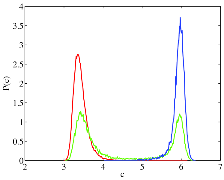
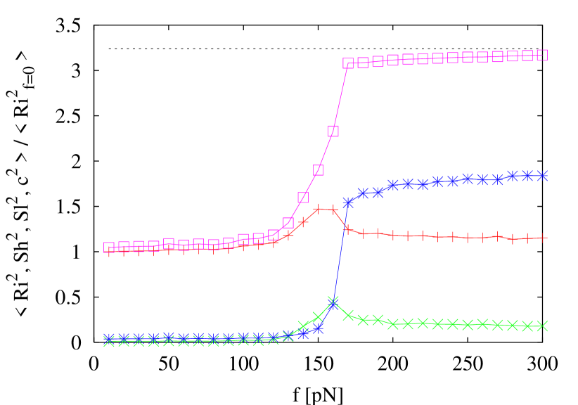
Figure 12: (Color online) (a) Probability distribution function of the center-center distance of successive base-pairs for $f=0\mbox{ (red)},\,140\mbox{ (green)},\,200\mbox{ (blue) pN}$. (b) Mean squared values of rise (red, plus), shift (green, crosses), slide (blue, stars), and center-of-mass distance (purple, squares) for neighboring base-pairs as a function of the stretching force $f$. The dashed line corresponds to the S-DNA center-of-mass distance. $\langle\mbox{Tw}\rangle$ of the resulting S-DNA conformation vanishes as predicted by Eq. (3).

The simulation results of the previous sections show several problems when this value of $\epsilon$ is chosen. First of all it cannot produce the correct persistence lengths, the chain is far to flexible. Secondly the undistorted ground state is not a B-DNA anymore. The thermal fluctuations suffice to unstack and untwist the chain locally. That is why one has to choose larger $\epsilon$ values even though the critical force is going to be overestimated.

Therefore we choose the following way to fix the parameter set $\{b,\epsilon,k\}$. First of all we choose a value for the stacking energy that reproduces correctly the persistence length. Afterwards the torsional persistence length is fixed to the experimentally known values by choosing an appropriate spring constant $k$. The depth of the base-pairs has also an influence on the persistence lengths of the chain. If the depth $b$ is decreased larger fluctuations for all three rotational parameters are gained such that the persistence lengths get smaller. Furthermore the geometric structure and the behavior under pulling is very sensitive to $b$. Too small values provoke non-B-DNA conformations or unphysical S-DNA conformations. We choose for $b$ a value of $11\mbox{\AA}$ for those reasons. For $\epsilon=20$ and $k=64$ a bending stiffness of $l_{p}=170\mbox{bp}$ and a torsional stiffness of $l_{n}=270\mbox{bp}$ are obtained close to the experimental values. We use this parameter set to simulate the corresponding stress-strain relation.

The simulated stress-strain curves for $50$ base-pairs show three different regimes (see Fig. 11). (i) For small stretching forces the WLC behavior of the DNA in addition with linear stretching elasticity of the backbones is recovered. This regime is completely determined by the chain length $N$. Due to the coarse-graining procedure that provides analytic expressions of the persistence lengths depending on the base-pair parameters (see eqs. (8),(11)) it is not necessary to simulate a chain of a few thousand base-pairs. The stress-strain relation of the entropic and WLC stretching regime (small relative extensions $L/L_{0}$ and small forces) is known analytically MarkoSiggia_mm_95 ; Odijk_mm_95 . Since we have parameterized the model in such a way that we recover the elastic properties of DNA on large length scales the simulation data for very long chains will follow the analytical result for small stretching forces. (ii) Around the critical force $f_{crit}\approx 140\mbox{pN}$ which is mainly determined by the stacking energy of the base-pairs the structural transition from B-DNA to S-DNA occurs. (iii) For larger forces the bonds become overstretched. Our MC simulations suggest a critical force $f_{crit}\approx 140\mbox{pN}$ which is slightly smaller than the value $f_{crit}\approx 180\mbox{pN}$ calculated by minimizing the energy. This is due to entropic contributions.

In order to further characterize the B-to-S-transition we measured the mean values of rise, slide, shift, etc. as a function of the applied forces. The evaluation of the MC data shows that the mean values of shift, roll and tilt are completely independent of the applied stretching force and vanish for all $f$. Rise increases at the critical force from the undisturbed value of $3.3\mbox{\AA}$ to approximately $4.0\mbox{\AA}$ and decays subsequently to the undisturbed value. Quite interestingly the mean value of slide jumps from its undisturbed value of $0$ to $\pm 5\mbox{\AA}$ (no direction is favored) and the twist changes at the critical force from $\pi/10$ to $0$. The calculation of the distribution function of the center-center distance $c$ of two neighboring base-pairs for $f=140\mbox{pN}$ yields a double-peaked distribution (see Fig. 12) indicating that part of the chain is in the B-form and part of the chain in the S-form. The contribution of the three translational degrees of freedom to the center-center distance $c$ is shown in Fig. 12. The S-DNA conformation is characterized by $\mbox{Ri}=3.3\mbox{\AA}$, $\mbox{Sl}=\pm 5\mbox{\AA}$ and $\mbox{Tw}=0$. In agreement with Refs. Cluzel_sci_96 ; Lavery_genetica_99 we obtain a conformation with highly inclined base-pairs still allowing for partial stacking of successive base-pairs.

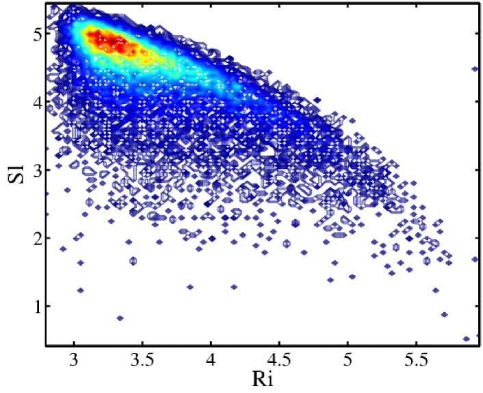
Figure 13: (Color online) Contour plot of rise [Å] versus slide [Å] for the S-DNA conformation.

V Discussion

We have introduced a simple model Hamiltonian describing double-stranded DNA on the base-pair level. Due to the simplification of the force-field and, in particular, the possibility of non-local MC moves our model provides access to much larger length scales than atomistic simulations. For example, $4h$ on a AMD Athlon MP 2000+ processor are sufficient in order to generate 1000 independent conformations for chains consisting of $N=100$ base-pairs.

In the data analysis, the main emphasis was on deriving the elastic constants on the elastic rod level from the analysis of thermal fluctuations of base-pair step parameters. Assuming a twisted ladder as ground state conformation one can provide an analytical relationship between the persistence lengths and the local elastic constants given by eqs. (8), (11) . Future work has to show, if it is possible to obtain suitable parameters for our mesoscopic model from a corresponding analysis of atomistic simulations Lavery_bpj_00 or quantum-chemical calculations bickelhaupt . In the present paper, we have chosen a top-down approach, i.e. we try to reproduce the experimentally measured behavior of DNA on length scales beyond the base diameter. The analysis of the persistence lengths, the mean and mean squared values of all six base-pair parameters and the critical force, where the structural transition from B-DNA to S-DNA takes place, as a function of the model parameters $\{b,k,\epsilon\}$ and the applied stretching force $f$ suggests the following parameter set:

$$2b =11\mbox{\AA}$$ (32)

$$\epsilon =20k_{B}T$$ (33)

$$k =64k_{B}T/\mbox{\AA}^{2}.$$ (34)

It reproduces the correct persistence lengths for B-DNA and entails the correct mean values of the base-pair step parameters known by X-ray diffraction studies. While the present model does not include the distinction between the minor and major groove and suppresses all internal degrees of freedom of the base-pairs such as propellor twist, it nevertheless reproduces some experimentally observed features on the base-pair level. For example, the anisotropy of the bending angles (rolling is easier than tilting) is just a consequence of the plate-like shape of the base-pairs and the twist-stretch coupling is the result of the preferred stacking of neighboring base-pairs and the rigid backbones.

The measured critical force is overestimated by a factor of $2$ and cannot be improved further by fine-tuning of the three free model parameters $\{b,k,\epsilon\}$. $f_{crit}$ depends solely on the stacking energy value $\epsilon$ that cannot be reduced further. Otherwise neither the correct equilibrium structure of B-DNA nor the correct persistence lengths would be reproduced. Our model suggests a structure for S-DNA with highly inclined base-pairs so as to enable at least partial base-pair stacking. This is in good agreement with results of atomistic B-DNA simulations by Lavery et al. Cluzel_sci_96 ; Lavery_genetica_99 . They found a force plateau of $140\mbox{pN}$ for freely rotating ends Cluzel_sci_96 . The mapping to the SOP model yields the following twist-stretch (Ri-Tw) coupling constant $k_{Ri,Tw}=({\cal C}^{-1})_{Ri,Tw}=267/\mbox{\AA}$. $k_{Ri,Tw}$ is the microscopic coupling of rise and twist describing the untwisting of the chain due to an increase of rise (compare also Fig. 6).

Possible applications of the present model include the investigation of (i) the charge renormalization of the WLC elastic constants podgornik , (ii) the microscopic origins of the cooperativity of the B-to-S transition Nelson_epl_03 , and (iii) the influence of nicks in the sugar-phosphate backbone on force-elongation curves. In particular, our model provides a physically sensible framework to study the intercalation of certain drugs or of ethidium bromide between base pairs. The latter is a hydrophobic molecule of roughly the same size as the base-pairs that fluoresces green and likes to slip between two base-pairs forming an DNA-ethidium-bromide complex. The fluorescence properties allow to measure the persistence lengths of DNA Schurr_arevpc_86 . It was also used to argue that the force plateau is the result of a DNA conformational transition Cluzel_sci_96 .

In the future, we plan to generalize our approach to a description on the base level which includes the possibility of hydrogen-bond breaking between complementary bases along the lines of Ref. Barbi_pl_99 ; Cocco_prl_99 . A suitably parameterized model allows a more detailed investigation of DNA unzipping experiments Heslot_prl_97 as well as a direct comparison between the two mechanism currently discussed for the B-to-S transition: the formation of skewed ladder conformations (as in the present paper) versus local denaturation Bloomfielda_bpj_01 ; Bloomfieldb_bpj_01 ; Bloomfieldc_bpj_01 . Clearly, it is possible to study sequence-effects and even more refined models of DNA. For example, it is possible to mimic minor and major groove by bringing the backbones closer to one side of the ellipsoids without observing non-B-DNA like ground states. The relaxation of the internal degrees of freedom of the base-pairs characterized by another set of parameters (propeller twist, stagger, etc.) should help to reduce artifacts which are due to the ellipsoidal shape of the base-pairs. Sequence effects enter via the strength of the hydrogen bonds ($E_{GC}=2.9k_{B}T$ versus $E_{AT}=1.3k_{B}T$) as well as via base dependent stacking interactions Hunter_jmb_92 . For example, one finds for guanine a concentration of negative charge on the major-groove edge whereas for cytosine one finds a concentration of positive charge on the major-groove edge. For adanine and thymine instead there is no strong joint concentration of partial charges CalladineDrew99 . It is known that in a solution of water and ethanol where the hydrophobic effect is less dominant these partial charges cause GG/CC steps to adopt A- or C-forms Fang_nar_99 by a negative slide and positive roll motion and a positive slide motion respectively. Thus by varying the ratio of the strengths of the stacking versus the electrostatic energy it should be possible to study the transition from B-DNA to A-DNA and C-DNA respectively.

VI Summary

Inspired by the results of El Hassan and Calladine ElHassanCalladine_ptrs_97 and of Hunter et al. HunterLu_jmb_97 ; Hunter_jmb_92 we have put forward the idea of constructing simplified DNA models on the base(-pair) level where discotic ellipsoids (whose stacking interactions are modeled via coarse-grained potentials ralf_GB ; Gay-Berne ) are linked to each other in such a way as to preserve the DNA geometry, its major mechanical degrees of freedom and the physical driving forces for the structure formation CalladineDrew99 .

In the present paper, we have used energy minimization and Monte Carlo simulations to study a simple representative of this class of DNA models with non-separable base-pairs. For a suitable choice of parameters we obtained a B-DNA like ground state as well as realistic values for the bend and twist persistence lengths. The latter were obtained by analyzing the thermal fluctuations of long filaments as well as by a systematic coarse-graining from the stack-of-plates to the elastic rod level. In studying the response of DNA to external forces or torques, models of the present type are not restricted to the regime of small local deformations. Rather by specifying a physically motivated Hamiltonian for arbitrary base-(step) parameters, our ansatz allows for realistic local structural transitions. For the simple case of a stretching force we observed a transition from a twisted helix to a skewed ladder conformation. While our results suggest a similar structure for S-DNA as atomistic simulations Cluzel_sci_96 , the DNA model studied in this paper can, of course, not be used to rule out the alternate possibility of local strand separations Bloomfielda_bpj_01 ; Bloomfieldb_bpj_01 ; Bloomfieldc_bpj_01 .

In our opinion, the base(-pair) level provides a sensible compromise between conceptual simplicity, computational cost and degree of reality. Besides providing access to much larger scales than atomistic simulations, the derivation of such models from more microscopic considerations provides considerable insight. At the same time, they may serve to validate and unify analytical approaches aiming at (averaged) properties on larger scales ChatenayMarko_pre_01 ; HZhou_prl_99 ; Barbi_pl_99 ; Cocco_prl_99 ; Nelson_epl_03 . Finally we note that the applicability of linked-ellipsoid models is not restricted to the base-pair level of DNA as the same techniques can, for example, also be used to study chromatin Wedemann_bpj_02 ; Katritch_jmb_00 ; mergell_prep .

VII Acknowledgments

We greatfully acknowledge extended discussions with K. Kremer, R. Lavery and A.C. Maggs. We thank H. Schiessel for a careful reading of our manuscript. Furthermore we are greatful to the DFG for the financial support of this work within the Emmy-Noether grant.

References

- (1) J. D. Watson and F. H. C. Crick, Nature 171, 737 (1953).
- (2) R. E. Dickerson et al., Science 216, 475 (1982).
- (3) R. E. Dickerson, Methods in Enzymology 211, 67 (1992).
- (4) T. L. James, Methods in Enzymology 261, 1 (1995).
- (5) D. P. Millar, R. J. Robbins, and A. H. Zewail, J. Chem. Phys. 76, 2080 (1982).
- (6) J. M. Schurr and K. S. Schmitz, Annual Review of Physical Chemistry 37, 271 (1986).
- (7) T. T. Perkins, S. Quake, D. Smith, and S. Chu, Science 264, 822 (1994).
- (8) T. C. Boles, J. H. White, and N. R. Cozzarelli, J. Mol. Biol. 213, 931 (1990).
- (9) S. B. Smith, L. Finzi, and C. Bustamante, Science 258, 1122 (1992).
- (10) S. B. Smith, Y. Cui, and C. Bustamante, Science 271, 795 (1996).
- (11) P. Cluzel et al., Science 264, 792 (1996).
- (12) B. Essevaz-Roulet, U. Bockelmann, and F. Heslot, Proc. Natl. Acad. Sci. USA 94, 11935 (1997).
- (13) J. Allemand, D. Bensimon, R. Lavery, and V. Croquette, Proc. Natl. Acad. Sci. USA 95, 14152 (1998).
- (14) C. R. Calladine and H. R. Drew, J. Mol. Biol. 178, 773 (1984).
- (15) R. E. Dickerson et al., EMBO Journal 8, 1 (1989).
- (16) X. J. Lu and W. K. Olson, J. Mol. Biol. 285, 1563 (1999).
- (17) W. K. Olson et al., J. Mol. Biol. 313, 229 (2001).
- (18) C. R. Calladine and H. R. Drew, Understanding DNA: The molecule and how it works, Academic Press, 1999.
- (19) J. F. Marko and E. D. Siggia, Macromolecules 27, 981 (1994).
- (20) J. F. Marko and E. D. Siggia, Macromolecules 28, 8759 (1995).
- (21) T. T. Perkins, D. E. Smith, R. G. Larson, and S. Chu, Science 268, 83 (1995).
- (22) N. R. Cozzarelli and J. C. Wang, DNA Topology and Its Biological Effects, Cold Spring Harbour Laboratory Press, Cold Spring Harbour, NY, 1990.
- (23) T. Schlick and W. K. Olson, J. Mol. Biol. 223, 1089 (1992).
- (24) G. Chirico and J. Langowski, Biopolymers 34, 415 (1994).
- (25) H. Schiessel, J. Widom, R. F. Bruinsma, and W. M. Gelbart, Phys. Rev. Lett. 86, 4414 (2001).
- (26) M. A. E. Hassan and C. R. Calladine, Proc. R. Soc. Lond. A 453, 365 (1997).
- (27) C. O’Hern, R. Kamien, T. Lubensky, and P. Nelson, Eur. Phys. J. B 1, 95 (1998).
- (28) A.Sarkar, J. F. Leger, D. Chatenay, and J. F. Marko, Phys. Rev. E 63, 051903 (2001).
- (29) Z. Haijun, Z. Yang, and O.-Y. Zhong-can, Phys. Rev. Lett. 82, 4560 (1999).
- (30) M. Barbi, S. Cocco, and M. Peyrard, Physics Letters A 253, 358 (1999).
- (31) S. Cocco and R. Monasson, Phys. Rev. Lett. 83, 5178 (1999).
- (32) N. Bruant, D. Flatters, R. Lavery, and D. Genest, Biophys. J. 77, 2366 (1999).
- (33) M. A. E. Hassan and C. R. Calladine, Phil. Trans. R. Soc. Lond. A 355, 43 (1997).
- (34) C. A. Hunter and X.-J. Lu, J. Mol. Biol. 265, 603 (1997).
- (35) C. A. Hunter, J. Mol. Biol. 230, 1025 (1993).
- (36) R. Everaers and M. R. Ejtehadi, Phys. Rev. E 67, 041710 (2003).
- (37) J. G. Gay and B. J. Berne, J. Chem. Phys. 74, 3316 (1981).
- (38) M. S. Babcock, E. P. D. Pednault, and W. K. Olson, J. Mol. Biol. 237, 125 (1994).
- (39) M. J. Packer and C. A. Hunter, J. Mol. Biol. 280, 407 (1998).
- (40) D. P. Landau and K. Binder, Monte Carlo Simulations in Statistical Physics, Cambridge University Press, 2000.
- (41) N. Metropolis, A. W. Rosenbluth, M. N. Rosenbluth, A. N. Teller, and E. Teller, J. Chem. Phys. 21, 1087 (1953).
- (42) T. R. Strick, D. Bensimon, and V. Croquette, Genetica 106, 57 (1999).
- (43) R. Lavery and A. Lebrun, Genetica 106, 75 (1999).
- (44) R. Lavery, A. Lebrun, J.-F. Allemand, D. Bensimon, and V. Croquette, J. Phys.: Condens. Matter 14, R383 (2002).
- (45) C. Bustamante, S. B. Smith, J. Liphardt, and D. Smith, Current Opinion in Structural Biology 10, 279 (2000).
- (46) D. Bensimon, D. Dohmi, and M. Mezard, Europhys. Lett. 42, 97 (1998).
- (47) J. Bednar et al., J. Mol. Biol. 254, 579 (1995).
- (48) M. Vologodskaia and A. Vologodskii, J. Mol. Biol. 317, 205 (2002).
- (49) R. D. Kamien, T. C. Lubensky, P. Nelson, and C. S. O’Hern, Europhys. Lett. 38, 237 (1997).
- (50) J. F. Marko, Europhys. Lett. 38, 183 (1997).
- (51) P. Nelson, Biophys. J. 74, 2501 (1998).
- (52) T. R. Strick, J.-F. Allemand, D. Bensimon, A. Bensimon, and V. Croquette, Science 271, 1835 (1996).
- (53) T. Odijk, Macromolecules 28, 7016 (1995).
- (54) I. Lafontaine and R. Lavery, Biophys. J. 79, 680 (2000).
- (55) C. F. Guerra and F. M. Bickelhaupt, Angewandte Chemie-International Edition 38, 2942 (1999).
- (56) R. Podgornik, P. L. Hansen, and V. A. Parsegian, J. Chem. Phys. 113, 9343 (2000).
- (57) C. Storm and P. Nelson, arXiv:physics/0212032 (2002).
- (58) U. Bockelmann, B. Essevaz-Roulet, and F. Heslot, Phys. Rev. Lett. 79, 4489 (1997).
- (59) M. C. Williams, J. R. Wenner, I. Rouzina, and V. A. Bloomfield, Biophys. J. 80, 874 (2001).
- (60) I. Rouzina and V. A. Bloomfield, Biophys. J. 80, 882 (2001).
- (61) I. Rouzina and V. A. Bloomfield, Biophys. J. 80, 894 (2001).
- (62) Y. Fang, T. S. Spisz, and J. H. Hoh, Nucleic Acids Research 27, 1943 (1999).
- (63) G. Wedemann and J. Langowski, Biophys. J. 82, 2847 (2002).
- (64) V. Katritch, C. Bustamante, and W. K. Olson, J. Mol. Biol. 295 (2000).
- (65) B. Mergell, H. Schiessel, and R. Everaers, in preparation.