Persistence properties of a system of coagulating and annihilating random walkers.

Abstract

We study a $d$-dimensional system of diffusing particles that on contact either annihilate with probability $1/(q-1)$ or coagulate with probability $(q-2)/(q-1)$. In $1$-dimension, the system models the zero temperature Glauber dynamics of domain walls in the $q$-state Potts model. We calculate $\bar{P}(m,t)$, the probability that a randomly chosen lattice site contains a particle whose ancestors have undergone exactly $(m-1)$ coagulations. Using perturbative renormalization group analysis for $d<2$, we show that, if the number of coagulations $m$ is much less than the typical number $M(t)$, then $\bar{P}(m,t)\sim m^{\zeta/d}t^{-\theta}$, with $\theta=dQ+Q(Q-1/2)\epsilon+O(\epsilon^{2})$, $\zeta=(2Q-1)\epsilon+(2Q-1)(Q-1)(1/2+AQ)\epsilon^{2}+O(\epsilon^{3})$, where $Q=\frac{q-1}{q}$, $\epsilon=2-d$ and $A=-0.006\ldots$. $M(t)$ is shown to scale as $M(t)\sim t^{d/2-\delta}$, where $\delta=d(1-Q)+(Q-1)(Q-1/2)\epsilon+O(\epsilon^{2})$. In two dimensions, we show that $\bar{P}(m,t)\sim\ln(t)^{Q(3-2Q)}\ln(m)^{(2Q-1)^{2}}t^{-2Q}$ for $m\ll t^{2Q-1}$. The $1$-dimensional results corresponding to $\epsilon=1$ are compared with results from Monte Carlo simulations.

I Introduction

Persistence is understood as a property of an evolving system to “remember” its initial configuration for anomalously long times. A particular case of persistence that has received much attention is that of site persistence (see SM for a review). The site persistence probability is defined as the probability that the values of a dynamical variable at a given set of sites do not change up to time $t$. For instance, in a spin system this could be the probability that a spin at a given site does not flip up to time $t$, or in a reaction-diffusion system, the probability that no reaction takes place at that site up to time $t$. In many cases the site persistence probability decays at large times as a power-law cardy1 .

A natural generalization of site persistence is persistence of a pattern present in the initial configuration MC . An instance of pattern persistence would be the survival of a test particle in a random environment. Examples of the random environment include diffusing traps DV ; MG , reaction-diffusion systems such as $A\emptyset\leftrightarrow\emptyset A$ DB1 , $A+B\rightarrow\emptyset$ DB1 ; BB or $A_{i}+A_{j}\rightarrow A_{i+j}$ with mass dependent diffusion rates alava1 ; alava2 ; KRZ1 , and predators in predator-prey models KR1 ; CK . The problem of calculating the survival probability of the test particle is hard, mainly because in the rest frame of the test particle, the motion of the other particles is correlated.

The $1$-dimensional Potts model has been a testing ground for various concepts of persistence. The site persistence problem mentioned above, has been exactly solved for the $1$-dimensional $q$-state Potts model evolving via zero temperature Glauber dynamics derrida . Besides site persistence, several other persistence properties of the Potts model have been studied. Among these are the probability that a domain wall has never encountered another domain wall monthus ; MC ; DB2 , and the probability that a domain present in the initial configuration survives up to time $t$ NK . The former problem has been studied numerically MC ; DB2 , by mean field approximations MC and perturbatively near $q=1$ monthus . However, the results obtained by these techniques do not approximate well the numerical results in the whole range of $q$.

In dimensions greater than one, the dynamics of domain walls in the Potts model is difficult to treat analytically. Instead, we note that in $1$-dimension, the zero temperature Glauber dynamics of the $q$-state Potts model is equivalent to a system of diffusing particles that on contact either annihilate with probability $1/(q-1)$ or coagulate with probability $(q-2)/(q-1)$ D ; satya ; SC . We study the persistence properties of this reaction-diffusion system in an arbitrary number of dimensions using the renormalization group method and calculate the exponents as an $\epsilon$-expansion.

The question that we ask is, given this reaction-diffusion system, what is the fraction of particles that have never encountered another particle up to time $t$? More generally, what is the fraction of particles whose ancestors have undergone $m$ coagulations up to time $t$? A convenient way to keep track of the history of coagulations is to assign a mass to each particle as follows. At time $t=0$, let all particles be of mass one. Each time two particles coagulate, the new particle has a mass which is the sum of the masses of the two parent particles. It is clear that the particles of mass $m$ will be those whose ancestors have undergone exactly $(m-1)$ coagulations.

Let $\bar{P}(m,t)$ be the probability that a randomly chosen site at time $t$ contains a particle of mass $m$. Let $\bar{N}(t)$ and $\bar{\rho}(t)$ denote the average particle density and average mass density respectively. Then, the probability distribution $\bar{P}(m,t)$ is expected to have the scaling form

$$\bar{P}(m,t)=\frac{\bar{N}(t)^{2}}{\bar{\rho}(t)}f\left(\frac{l_{m}}{\sqrt{t}}\right),$$ (1)

where $l_{m}=(m/\bar{\rho}(t))^{1/d}$ is the length scale associated with mass. The large time behavior of $\bar{\rho}(t)$ and $\bar{P}(m,t)$ is characterized by two exponents $\delta$ and $\theta$. The mass density $\bar{\rho}(t)\sim t^{-\delta}$. For masses much smaller than the typical mass, $\bar{P}(m,t)$ decays as a power law in time as $m^{\zeta/d}t^{-\theta}$. We will call $\theta$ the persistence exponent. The exponent $\zeta$ characterizes the small $x$ behavior of the scaling function $f(x)$ to be $f(x)\sim x^{\zeta}$ for $x\ll 1$. Then, $\zeta=2d(\theta+\delta-d)/(d-2\delta)$, where we have used the fact that $\bar{N}(t)\sim t^{-d/2}$ in dimensions less than two Peliti . The two independent exponents $\theta$ and $\delta$ are known for some limiting cases.

When $q=2$, the model reduces to the reaction diffusion model $A+A\rightarrow\emptyset$. All particles are of mass one and it is known that $\bar{P}(1,t)\sim t^{-d/2}$ for $d<2$ and $\bar{P}(1,t)\sim\ln(t)/t$ for $d=2$ aa ; Peliti . Hence, $\delta=d/2$, $\theta=d/2$ and $\zeta=0$ for $q=2$. When $q=\infty$, the model is equivalent to the reaction-diffusion system $A_{i}+A_{j}\rightarrow A_{i+j}$ spouge ; bram ; KR ; satya ; oleg ; KRZ1 . Since mass is conserved, $\delta=0$. It has been shown that $\theta=d+\epsilon/2+O(\epsilon^{2})$, and $\zeta=\epsilon+O(\epsilon^{2})$ for $\epsilon=2-d>0$ KRZ1 . In $2$-dimensions $\bar{P}(m,t)\sim\ln(m)\ln(t)/t$ KRZ1 . In $1$-dimension, it is known via an exact calculation that $\bar{P}(m,t)\sim mt^{-3/2}$ spouge . When $q\approx 1$, $\theta$ has been calculated perturbatively to be $\theta=(q-1)3\sqrt{3}/(2\pi)+O((q-1)^{2})$ monthus . However for arbitrary values of $q$, the only known analytical result follows from a mean field approximation MC . But the numerically obtained value for $\theta$ is very different from the mean field value. In this paper, we address this issue by using the renormalization group formalism to systematically calculate $\bar{P}(m,t)$ for arbitrary $q$.

We now summarize our main results and give an outline of the rest of the paper. In Sec. II, we give a precise definition of the model and derive the stochastic partial differential equations obeyed by the mass distribution. In Sec. III we express the exponent $\delta$ in terms of the exponent $\theta$, though at a different value of $q$, reducing the number of unknown exponents to one. We show that

$$\delta(q)=\theta\left(\frac{q}{q-1}\right).$$ (2)

Thus,

$$\zeta(q)=\frac{2d\left[\theta(q)+\theta\left(\frac{q}{q-1}\right)-d\right]}{d-2\theta\left(\frac{q}{q-1}\right)}.$$ (3)

In Sec. IV we use the technique developed in KRZ1 to calculate the persistence exponent $\theta$ as an $\epsilon$-expansion, where $\epsilon=2-d>0$. We show that

$$\theta=dQ+Q(Q-\frac{1}{2})\epsilon+O(\epsilon^{2}),$$ (4)

where $Q=\frac{q-1}{q}$. If $d=2$, the scaling form Eq. (1) breaks down due to logarithmic corrections. We calculate these corrections to be

$$\bar{P}(m,t)\sim\frac{\ln(t)^{Q(3-2Q)}\ln(m)^{(2Q-1)^{2}}}{t^{2Q}},$$ (5)

given that $t\rightarrow\infty$ and $m\ll M(t)$, where $M(t)$ is mass of a typical particle at time $t$. The analytical results for $\theta$ and $\delta$ in $1$-dimension obtained by putting $\epsilon=1$ are compared with the results from numerical simulations.

In Sec. V we show that the coefficient of $\epsilon^{n}$ in Eq. (4) is a polynomial of degree $2n$ in the variable $Q=(q-1)/q$. This observation allows us to calculate the $2$-loop corrections to the exponent $\zeta$ to be

$$\zeta=(2Q-1)\epsilon+(2Q-1)(Q-1)(\frac{1}{2}+AQ)\epsilon^{2}+O(\epsilon^{3}),$$ (6)

where $A=-0.006\ldots$. The analytical results for $\zeta$ in $1$-dimension obtained by putting $\epsilon=1$ are compared with the results from numerical simulations.

Finally, we conclude with a summary and discussion in Sec. VI.

II Model and field theoretic formulation

In this section, we define the model and derive the stochastic partial differential equation obeyed by the mass distribution. Consider a $d$-dimensional lattice whose sites may be occupied by particles that possess a positive integral mass. Multiple occupancy of a lattice site is allowed. Given a certain configuration of particles on this lattice, the system evolves in time via the following microscopic moves. (i) With rate $D$, each particle hops to a nearest neighbor lattice site. (ii) With rate $\lambda_{c}$, two particles at the same site coagulates together to form a new particle whose mass is the sum of the masses of the two parent particles. (iii) With rate $\lambda_{a}$, two particles at the same site annihilate each other. To make connection with the model discussed in the introduction, we have to choose $\lambda_{c}=\lambda(q-2)/(q-1)$ and $\lambda_{a}=\lambda/(q-1)$ where $\lambda$ is a reaction rate. The limit $\lambda\rightarrow\infty$ corresponds to instantaneous reactions. In dimensions $d\leq 2$ and in the limit of large time, the statistical properties of a finite reaction rate particle system were shown to be equivalent to those of a system with infinite reaction rates KRZ1 . However, from the field theoretic point of view, it is more convenient to work with finite reaction rates, and hence $\lambda$ will be taken to be finite in this paper.

Starting from the master equation for the time evolution of the system, we now derive the effective field theory of the model. Let $\{n_{i}\}$ denote the configuration of particles at site $i$ such that $n_{i,m}$ is the number of particles of mass $m$ at site $i$. Let ${\mathcal{P}}(\ldots\{n_{i}\},\{n_{j}\},\ldots;t)$ be the probability of the configuration $(\ldots\{n_{i}\},\{n_{j}\},\ldots)$ at time $t$, where $i$ and $j$ are nearest neighbors. The master equation describing the time evolution of ${\mathcal{P}}(\ldots\{n_{i}\},\{n_{j}\},\ldots;t)$ is

$$\frac{d{\mathcal{P}}(\ldots\{n_{i}\},\{n_{j}\},\ldots)}{dt}=-D\sum_{\langle ij\rangle}\bigg{[}\sum_{m}(n_{i,m}+n_{j,m}){\mathcal{P}}(\{n_{i}\},\{n_{j}\})-\sum_{m}(n_{i,m}+1){\mathcal{P}}(\{n_{i,m}+1\},\{n_{j,m}-1\})$$ (7)

$$\mbox{}-\sum_{m}(n_{j,m}+1){\mathcal{P}}(\{n_{i,m}-1\},\{n_{j,m}+1\})\bigg{]}-\lambda_{c}\sum_{i}\bigg{[}\sum_{m\neq m^{\prime}}n_{i,m}n_{i,m^{\prime}}{\mathcal{P}}(\{n_{i}\})+\sum_{m}n_{i,m}(n_{i,m}-1){\mathcal{P}}(\{n_{i}\})$$

$$\mbox{}-\!\!\!\sum_{m\neq m^{\prime}}\!\!\!(n_{i,m}+1)(n_{i,m^{\prime}}+1){\mathcal{P}}(\{n_{i,m}+1,n_{i,m^{\prime}}+1,n_{i,m+m^{\prime}}\!-\!1\})-\sum_{m}(n_{i,m}+2)(n_{i,m}+1){\mathcal{P}}(\{n_{i,m}+2,n_{i,2m}\!-\!1\})\bigg{]}$$

$$\mbox{}-\lambda_{a}\sum_{i}\bigg{[}\sum_{m\neq m^{\prime}}n_{i,m}n_{i,m^{\prime}}{\mathcal{P}}(\{n_{i}\})+\sum_{m}n_{i,m}(n_{i,m}-1){\mathcal{P}}(\{n_{i}\})-\!\!\!\sum_{m\neq m^{\prime}}\!\!\!(n_{i,m}+1)(n_{i,m^{\prime}}+1){\mathcal{P}}(\{n_{i,m}+1,n_{i,m^{\prime}}+1\})$$

$$\mbox{}-\sum_{m}(n_{i,m}+2)(n_{i,m}+1){\mathcal{P}}(\{n_{i,m}+2\})\bigg{]},$$

where the time dependence of ${\mathcal{P}}$ has been dropped for notational simplicity and $\{n_{i,m}+1\}$ denotes the configuration $(n_{i,1},n_{i,2},\ldots,n_{i,m}+1,\ldots)$ at site $i$. The first term in the right hand side of Eq. (7) describes the loss and gain terms arising from particles diffusing to their nearest neighbors with rate $D$. The second term describes the loss and gain terms due to the coagulation of a pair of particles at a site with rate $\lambda_{c}$ to form a new particle whose mass is the sum of the constituents. The third term describes the loss and gain terms due to annihilation of a pair of particles at a site with rate $\lambda_{a}$.

The field theory corresponding to the problem can be derived from the master equation using Doi’s formalism Doi . In short, regarding the master equation as a Schroedinger equation in imaginary time, the functional integral representation of the corresponding non-Hermitian evolution operator is constructed. This allows one to write down a functional integral expression for any correlation function of the problem, including $\bar{P}(m,t)$. After taking the continuum limit, one is left with the problem of solving an interacting field theory. The application of Hubbard-Stratonovich transformation to this field theory leaves one with a stochastic partial differential equation. We refer to Refs. cardy ; oleg ; mattis for reviews of this procedure. Following this procedure, solving the master equation Eq. (7) is equivalent to solving the following Langevin equation for a stochastic field $\tilde{P}(\vec{x},m,t)$:

$$(\partial_{t}-D\nabla^{2})\tilde{P}(\vec{x},m,t)=$$ (8)

$$\mbox{}-2(\lambda_{c}+\lambda_{a})\tilde{P}(\vec{x},m,t)\int_{0}^{\infty}dm^{\prime}\tilde{P}(\vec{x},m^{\prime},t)+\lambda_{c}\tilde{P}*\tilde{P}$$

$$\mbox{}+i\sqrt{2(\lambda_{a}+\lambda_{c})}\xi(\vec{x},t)\tilde{P}(\vec{x},m,t),$$

where $\tilde{P}*\tilde{P}=\int_{0}^{m}dm^{\prime}\tilde{P}(\vec{x},m^{\prime},t)\tilde{P}(\vec{x},m-m^{\prime},t)$, $\xi$ is white noise in space and time with unit standard deviation and $i^{2}=-1$.

The stochastic field $\tilde{P}(\vec{x},m,t)$ is complex and is different from the local mass distribution $P(\vec{x},m,t)$, which denotes the number of particles of mass $m$ in the volume $d^{d}xdm$ at time t. However, the moments of $P$ are related to the moments of $\tilde{P}$ (for instance, see mattis ; Lee ). For example, $\overline{P(\vec{x},m,t)}=\overline{\tilde{P}(\vec{x},m,t)}$, $\overline{P(\vec{x},m,t)^{2}}=\overline{\tilde{P}(\vec{x},m,t)}(\Delta m(\Delta x)^{d})^{-1}+\overline{\tilde{P}(\vec{x},m,t)^{2}}$, and so on, where the bar on top denotes an averaging over noise, and $\Delta x$ and $\Delta m$ are lattice cutoffs. In this paper we only study the first moment of $P(\vec{x},m,t)$, and hence disregard the difference between $P(\vec{x},m,t)$ and $\tilde{P}(\vec{x},m,t)$ in the rest of the paper.

We will be studying the behavior of the following three quantities,

$$P(m,\vec{x},t) m\ll M(t),$$ for (9)

$$N(\vec{x},t) = \int_{0}^{\infty}dmP(m,\vec{x},t),$$ (10)

$$\rho(\vec{x},t) = \int_{0}^{\infty}dm~{}mP(m,\vec{x},t),$$ (11)

where $N(\vec{x},t)$ is the local particle density, $\rho(\vec{x},t)$ is the local mass density and $M(t)\sim\bar{\rho}(t)/\bar{N}(t)$ is the typical mass at time $t$. The time evolution equations obeyed by $N(\vec{x},t)$ and $\rho(\vec{x},t)$ are easily obtained from Eq. (8). As for $P(m,\vec{x},t)$, for $m\ll M(t)$, we neglect the convolution term in the right hand side of Eq. (8). This approximation is justified because at large times the probability of collision of two light particles is negligible compared to the probability of collision of light and heavy particles. The resulting equations are:

$$(\partial_{t}-D\nabla^{2})N(\vec{x},t)=-(\lambda_{c}+2\lambda_{a})N(\vec{x},t)^{2}$$ (12)

$$\mbox{}+i\sqrt{2(\lambda_{a}+\lambda_{c})}\xi(\vec{x},t)N(\vec{x},t),$$

$$\!\!\!\!(\partial_{t}-D\nabla^{2})P(\vec{x},m,t)=-2(\lambda_{c}+\lambda_{a})P(\vec{x},m,t)N(\vec{x},t)$$ (13)

$$\mbox{}\!\!\!\!\!\!\!+i\sqrt{2(\lambda_{c}+\lambda_{a})}\xi(\vec{x},t)P(\vec{x},m,t),$$

$$(\partial_{t}-D\nabla^{2})\rho(\vec{x},t)=-2\lambda_{a}\rho(\vec{x},t)N(\vec{x},t)$$ (14)

$$\mbox{}+i\sqrt{2(\lambda_{c}+\lambda_{a})}\xi(\vec{x},t)\rho(\vec{x},t).$$

Note that the dependence of $P$ on mass is no longer governed by Eq. (13). Once the time dependence of $\bar{P}$ is calculated, its mass dependence can be restored using dimensional analysis. In the rest of the paper, for the sake of notational simplicity, we omit the dependence of $P$ on mass, unless there is a cause for confusion.

Equations (12), (13) and (14) can be simplified as follows. Let

$$\lambda_{c} = \frac{q-2}{q-1}\lambda,$$ (15)

$$\lambda_{a} = \frac{1}{q-1}\lambda$$ (16)

for some parameter $\lambda$. Rescaling the local particle density, local mass distribution and average density according to

$$\bigg{(}N(\vec{x},t),P(\vec{x},t),\rho(\vec{x},t)\bigg{)}\longrightarrow$$ (17)

$$\left(\frac{q-1}{q}\right)\bigg{(}N(\vec{x},t),P(\vec{x},t),\rho(\vec{x},t)\bigg{)},$$

brings Eqs. (12)–(14) into the following form:

$$(\partial_{t}-D\nabla^{2})N(\vec{x},t) = -\lambda N^{2}(\vec{x},t)$$ (18)

$$\mbox{}+i\sqrt{2\lambda}\xi(\vec{x},t)N(\vec{x},t),$$

$$(\partial_{t}-D\nabla^{2})P(\vec{x},t) = -2Q\lambda P(\vec{x},t)N(\vec{x},t)$$ (19)

$$\mbox{}+i\sqrt{2\lambda}\xi(\vec{x},t)P(\vec{x},t),$$

$$(\partial_{t}-D\nabla^{2})\rho(\vec{x},t) = -2(1-Q)\lambda\rho(\vec{x},t)N(\vec{x},t)$$ (20)

$$\mbox{}+i\sqrt{2\lambda}\xi(\vec{x},t)\rho(\vec{x},t),$$

where

$$Q=\frac{q-1}{q}.$$ (21)

It can be shown that Eqs. (18) and (19) describe the two species reaction $A+A\stackrel{{\scriptstyle\lambda}}{{\rightarrow}}A$, $A+B\stackrel{{\scriptstyle Q\lambda}}{{\rightarrow}}\emptyset$, in the limit when the concentration of $A$-particles is much greater than concentration of $B$-particles.

III Scaling analysis of stochastic evolution equations.

In this section, we obtain some exact results for the model. First, the scaled density of particles $N(\vec{x},t)$ obeys the same equation as the particle density in the $A+A\rightarrow A$ reaction. For this reaction, the density of particles decays for large times as $t^{-d/2}$ in $d<2$ aa ; Peliti . Thus,

$$N(t)=c\frac{q-1}{q}\frac{1}{t^{d/2}},~{}t\rightarrow\infty,$$ (22)

where $c$ is a constant depending on dimension only. This is a generalization of the exact $1$-dimensional result zeitak ; masser .

Secondly, there is a relation between the local mass distribution of light particles $P$ and the local mass density $\rho$. Under the substitution $Q\rightarrow(1-Q)$, or equivalently $q/(q-1)\rightarrow q$, Eq. (19) transforms into Eq. (20). Therefore, if $F_{P}(Q,\vec{x}_{1},t_{1},\vec{x}_{2},t_{2},\ldots)$ is a correlation function of $P$-fields, which is independent of initial conditions, then $F_{P}(1-Q,\vec{x}_{1},t_{1},\vec{x}_{2},t_{2},\ldots)$ is the correlation function of the same configuration of $\rho$-fields. In particular, since $\bar{P}(t)\sim t^{-\theta(Q)}$, we obtain $\rho(t)\sim t^{-\theta(1-Q)}$. Thus, we derive Eq. (2), namely

$$\delta(Q)=\theta(1-Q).$$ (23)

We now examine Eqs. (18) and (19) for special values of the parameter $Q$. When $Q=0$, the non-linear term in Eq. (19) vanishes and the concentration of monomers is conserved on average. Therefore, $\theta=0$ for $Q=0$. When $Q=1/2$, Eq. (19) is solved by $P\sim N$, where $N$ is a solution of Eq. (18). Then, from Eq. (22), we obtain $\theta=d/2$ for $Q=1/2$. When $Q=1$, it is known that $\theta=d+\epsilon/2+O(\epsilon^{2})$, where $\epsilon=2-d$ KRZ1 . If $d=1$, then $\theta=3/2$, which is a consequence of an exact solution spouge , rather than the $\epsilon$-expansion cited above. Collecting these results together, we have

$$\theta=\cases{0&for $Q=0$,\cr\frac{d}{2}&for $Q=\frac{1}{2}$,\cr d+\frac{\epsilon}{2}+O(\epsilon^{2})&for $Q=1$.\cr}$$ (24)

The question remains as to whether $\theta$ for $Q<1/2$ or equivalently $q<2$ has any physical implication. For the site persistence problem in $1$-dimension, it is known that the site persistence probability of the $q$-state Potts model maps to an Ising system with an initial magnetization given by $2/q-1$, evolving via zero-temperature Kawasaki dynamics satya ; SC ; BFK . The latter system is defined at any value of $q>1$. The correspondence between these two models also holds for the persistence probability of a single domain in the Potts model NK . It would be interesting to understand what quantity, if any, in the Ising model corresponds to the survival probability of domain walls in the Potts model.

IV Perturbative computation of persistence exponent near $d=2$.

In this section, we calculate the large time behavior of $\bar{P}(t)$ using the formalism of perturbative renormalization group. We closely follow the solution of the $A_{i}+A_{j}\rightarrow A_{i+j}$ model presented in Ref. KRZ1 .

The solution to $\bar{P}(t)$ as a perturbative expansion in powers of $\lambda$ can be constructed from Eqs. (18) and (19) using Feynman diagrams Drouffe . The Feynman rules for constructing terms of the expansion are summarized in Fig. 1. Diagrammatically, $\bar{P}$ and $\bar{N}$ are the sum of all Feynman diagrams with one outgoing $P$ and $N$ line respectively. Clearly, there are an infinite number of diagrams contributing to $\bar{P}$ and $\bar{N}$. These diagrams can be grouped together according to the number of loops that they contain, thus giving rise to the loop expansion. Let $\epsilon=2-d$. The contribution from each diagram is a function of the dimensionless terms $\lambda N_{0}t$ and $g(t)=\lambda t^{\epsilon/2}$ and a term that gives the correct physical dimension [$(\lambda t)^{-1}$ for $\bar{N}$ and $(\lambda t)^{-2}$ for $\bar{P}$]. A simple combinatorial argument shows that the contribution from a diagram with $n$ loops is proportional to $g(t)^{n}$ Lee . When $\epsilon<0$, the main contribution to $\bar{P}$ and $\bar{N}$ comes from properly renormalized tree level diagrams (diagrams without loops) footnote . When $\epsilon>0$, the loop expansion fails since for large times $g(t)$ is no longer a small perturbation parameter. We therefore conclude that $2$ is the upper critical dimension. For $d<2$ we will use the formalism of perturbative renormalization group to convert the loop expansion into an $\epsilon$-expansion and calculate scaling exponents as a series in $\epsilon$.

Figure 1: Propagators and vertices of the theory.

IV.1 Tree level diagrams

Let $\bar{N}_{\rm{mf}}$ and $\bar{P}_{\rm{mf}}$ be mean field densities given by the sum of contributions coming from tree diagrams with a single outgoing $N$-line and $P$-line respectively. We denote $\bar{N}_{\rm{mf}}$ and $\bar{P}_{\rm{mf}}$ by thick solid lines and thick dashed lines respectively. The integral equations satisfied by $\bar{N}_{\rm{mf}}$ and $\bar{P}_{\rm{mf}}$ are presented in diagrammatic form in Fig. 2(a) and 2(b). After differentiating with respect to time, they can be written in analytic form as

$$\partial_{t}\bar{P}(t) = -2Q\lambda\bar{P}(t)\bar{N}(t),$$ (25)

$$\partial_{t}\bar{N}(t) = -\lambda\bar{N}^{2}(t),$$ (26)

in which one can easily recognize the Smoluchowski rate equations of the model, obtained from Eqs. (18) and (19) by neglecting the noise terms in the right hand side.

Equations (25) and (26) are easily solved yielding

$$\bar{N}_{\rm{mf}}(t) = \frac{N_{0}}{1+\lambda N_{0}t},$$ (27)

$$\bar{P}_{\rm{mf}}(t) = \frac{P_{0}}{(1+\lambda N_{0}t)^{2Q}}.$$ (28)

From Eq. (28), we obtain

$$\theta_{\rm{mf}}=2Q.$$ (29)

where $\theta_{\rm{mf}}$ is the mean field answer for $\theta$.

Figure 2: Diagrammatic form of mean field equations for (a) mean particle density $\bar{N}$, (b) mean density of mass $1$ particles $\bar{P}$, (c) $G_{\rm{mf}}^{\rm{NN}}$, and (d) $G_{\rm{mf}}^{\rm{PP}}$.

In calculating loop corrections to any given order, we are faced with the problem of summing over infinitely many diagrams containing a given number of loops. This problem can be simplified by introducing mean field propagators which are sums of all tree diagrams with one incoming line and one outgoing line. Expressed in terms of these mean field propagators, there are only finitely many diagrams with a fixed number of loops.

Let $G_{\rm{mf}}^{\rm{NN}}$ and $G_{\rm{mf}}^{\rm{PP}}$ be mean field propagators. The integral equations satisfied by them are presented in diagrammatic form in Figs. 2(c) and 2(d). The solutions to these equations are

$$G_{\rm{mf}}^{\rm{NN}}(2|1) = \left(\frac{\bar{N}_{\rm{mf}}(t_{2})}{\bar{N}_{\rm{mf}}(t_{1})}\right)^{2}G_{0}(2|1),$$ (30)

$$G_{\rm{mf}}^{\rm{PP}}(2|1) = \left(\frac{\bar{N}_{\rm{mf}}(t_{2})}{\bar{N}_{\rm{mf}}(t_{1})}\right)^{2Q}G_{0}(2|1),$$ (31)

where $1=(\vec{x}_{1},t_{1})$, $2=(\vec{x}_{2},t_{2})$ and $G_{0}$ is the Green’s function of the linear diffusion equation.

IV.2 One loop diagrams

Using the mean field propagators and densities, it is easy to classify all one loop diagrams contributing to $\bar{P}(t)$. These are shown in Fig. 3. The computation of the corresponding Feynman integrals is straightforward. The contributions from one-loop diagrams in the limit $N_{0}\rightarrow\infty$ are

$$(a) = \frac{32Q\lambda P_{0}t^{\epsilon/2}}{(8\pi)^{d/2}(N_{0}\lambda t)^{2Q}\epsilon^{2}(\epsilon+2)},$$ (32)

$$(b) = \frac{-64Q^{2}\lambda P_{0}t^{\epsilon/2}}{(8\pi)^{d/2}(N_{0}\lambda t)^{2Q}\epsilon(\epsilon+2)(\epsilon+4)},$$ (33)

$$(c) = \frac{-256Q\lambda P_{0}t^{\epsilon/2}}{(8\pi)^{d/2}(N_{0}\lambda t)^{2Q}\epsilon^{2}(\epsilon+2)^{2}(\epsilon+4)},$$ (34)

where $(a)$, $(b)$ and $(c)$ refer to the contributions from diagrams in Figs. 3(a), 3(b) and 3(c) respectively. Adding these one-loop contributions to the mean field answer Eq. (28), we obtain in the limit $N_{0}\rightarrow\infty$,

$$\bar{P}(t)=\frac{A}{t^{2Q}}+\frac{32Q\lambda A}{(8\pi)^{d/2}\epsilon t^{2Q-\epsilon/2}}\left[\frac{\epsilon+6-2Q(\epsilon+2)}{(\epsilon+2)^{2}(\epsilon+4)}\right]$$ (35)

$$\mbox{}+\mbox{$2$- and higher loop corrections,}$$

where $A=P_{0}/(N_{0}\lambda)^{2Q}$.

Figure 3: One loop corrections to the mean field result for $\bar{P}$.

IV.3 Renormalization Group Analysis of the Model.

The large time asymptotic behavior of $\bar{P}(t)$ can be obtained by solving the Callan-Symanzik equation with initial conditions given by Eq. (35) (see Ref. cardy for a review). The coefficients of Callan-Symanzik equation are determined by the law of renormalization of all the relevant couplings of the theory Eqs. (18) and (19). Power counting analogous to that carried out in KRZ1 , shows that there are only two relevant couplings of the theory in $d<2$: the reaction rate $\lambda$ and the initial mass distribution $P_{0}$. We will derive the one-loop renormalization law of the initial mass distribution by requiring that Eq. (35) is non-singular in the limit $\epsilon\rightarrow 0$ if expressed in terms of renormalized relevant couplings.

Let $t_{0}$ be a reference time and $g_{0}=\lambda t_{0}^{\epsilon/2}$ be the dimensionless reaction rate. We choose $t_{0}$ in such a way that $g_{0}\ll 1$. The mechanism of renormalization of the reaction rate in the theory is identical to that of the reaction $A+A\rightarrow A$. Physically, the renormalization of reaction rate is explained by the recurrent property of random walks. The probability of a reaction between particles at time $t$ is proportional to the ”bare” reaction rate, multiplied by the probability that the reaction has not occurred before time $t$. In $d\leq 2$, the latter probability explicitly depends on time $t$. The law of renormalization of the reaction rate has been worked out in Ref. Peliti . If $g_{R}$ is the renormalized reaction rate, then it is related to $g_{0}$ by the relation

$$g_{R}=\frac{g_{0}}{1+g_{0}/g^{*}},$$ (36)

where $g^{*}=2\pi\epsilon+O(\epsilon^{2})$ is the nontrivial fixed point of the renormalization group flow in the space of effective coupling constants. The mass distribution $\bar{P}(t_{0})$ can now be expressed in terms of the renormalized reaction rate $g_{R}$ to be

$$\bar{P}(t_{0})=\frac{P_{0}}{(N_{0}g_{R}t_{0}^{d/2})^{2Q}}\left[1-\frac{g_{R}}{g^{*}}Q(2Q-1)+O(g_{R}^{2})\right].$$ (37)

The order $g_{R}$ term in Eq. (37) is singular at $\epsilon=0$. To cancel this divergence, we have to introduce a renormalized initial mass distribution $P_{R}$:

$$P_{R}=Z(g_{R},t_{0},\epsilon)P_{0},$$ (38)

where $Z(g_{R},t_{0},\epsilon)$ is chosen such that

$$\bar{P}(t,g_{R},P_{R},t_{0})=Z(g_{R},t_{0},\epsilon)\bar{P}(t,\lambda,P_{0},\epsilon),$$ (39)

is non-singular at $\epsilon=0$. Substituting Eq. (39) into Eq. (37), we obtain

$$Z=1+\frac{g_{R}}{g^{*}}Q(2Q-1)+O(g_{R}^{2}).$$ (40)

The Callan-Symanzik equation is obtained by noting that $\bar{P}(t,\lambda,P_{0},\epsilon)$ does not depend on the reference time $t_{0}$. Therefore,

$$t_{0}\frac{\partial}{\partial t_{0}}\left[Z^{-1}\bar{P}(P_{R})\right]=0.$$ (41)

It follows from dimensional analysis that the most general form of the average mass distribution is

$$\bar{P}(t)=\frac{1}{t_{0}^{dQ}}\frac{P_{R}}{N_{0}^{2Q}}\Phi\left(\frac{t}{t_{0}},g_{R}\right),$$ (42)

where $\Phi$ is a dimensionless function. Using the scaling function Eq. (42) in Eq. (41), we obtain the Callan-Symanzik equation for $\bar{P}(t)$:

$$\left(t\frac{\partial}{\partial t}+\frac{\beta(g_{R})}{2}\frac{\partial}{\partial g_{R}}+dQ-\frac{\gamma(g_{R})}{2}\right)\bar{P}(t,g_{R},P_{R},t_{0})=0,$$ (43)

where

$$\beta(g_{R}) = -2t_{0}\frac{\partial g_{R}}{\partial t_{0}}=\frac{g_{R}(g_{R}-g^{*})\epsilon}{g^{*}},$$ (44)

$$\gamma(g_{R}) = \frac{-2t_{0}}{Z}\frac{\partial Z}{\partial t_{0}}=\frac{-2Q(2Q-1)}{4\pi}g_{R}+O(g_{R}^{2}),$$ (45)

are the beta and gamma functions of the theory.

At large times, the solutions of Eq. (43) are governed by the nontrivial fixed point $g^{*}$ of the beta function. It then follows from the Callan-Symanzik Eq. (43) that $\bar{P}(t)\sim t^{-\theta}$ where

$$\theta=Qd-\frac{\gamma(g^{*})}{2}.$$ (46)

Thus we obtain from Eqs. (45) and (46) that

$$\theta=dQ+Q(Q-\frac{1}{2})\epsilon+O(\epsilon^{2}),~{}\epsilon>0.$$ (47)

The knowledge of $\theta$ to the first order in $\epsilon$ combined with Eqs. (2) and (3) allows one to calculate the exponents $\delta$ and $\zeta$ with the same precision:

$$\delta = d(1-Q)+(Q-\frac{1}{2})(Q-1)\epsilon+O(\epsilon^{2}),$$ (48)

$$\zeta = (2Q-1)\epsilon+O(\epsilon^{2}).$$ (49)

The exponent $\zeta$ is proportional to the sum of the anomalous dimensions of $P$ and $\rho$. As a result, the mass dependence of $\bar{P}(m,t)$ can be captured neither by mean field theory nor by Smoluchowski approximation (see KRZ1 for a more detailed discussion of this point).

The results of this subsection can be summarized as follows. The mean mass distribution $\bar{P}(m,t)$ varies as

$$\bar{P}(m,t)\sim\frac{(m^{1/d})^{(2Q-1)\epsilon+O(\epsilon^{2})}}{t^{dQ+Q(Q-1/2)\epsilon+O(\epsilon^{2})}},$$ (50)

for $m\ll M(t)$, where $M(t)$ is the typical mass at time $t$, or equivalently the typical number of coagulations undergone by all ancestors of survived particles. $\bar{P}(m,t)$ decays algebraically with time with an exponent independent of $m$. The coefficient multiplying this time dependent term does however grow algebraically with $m$.

IV.4 Two dimensions.

The upper critical dimension of our model is $2$. The non-trivial fixed point of the $\beta$-function Eq. (44) vanishes at $d\rightarrow 2$. We therefore expect the mean field answers Eqs. (27) and (28) to give the correct large time-small mass of average densities in two dimension, modulo logarithmic corrections. In this subsection we calculate these corrections.

When $Q=1$ it was shown that in two dimensions, $\bar{P}(m,t)\sim\ln(t)\ln(m)t^{-2}$ for $t\rightarrow\infty,m\ll M(t)$ KRZ1 . To calculate these corrections for arbitrary $Q$ we need to solve the Callan-Symanzik equation (43) with coefficients calculated at $d=2$. In two dimensions,

$$\beta(g)|_{d=2} = \frac{g^{2}}{2\pi},$$ (51)

$$\gamma(g)|_{d=2} = \frac{-2Q(2Q-1)g}{4\pi}+O(g^{2}).$$ (52)

Then Eq. (43) reduces to

$$\left(t\frac{\partial}{\partial t}+\frac{g_{R}^{2}}{4\pi}\frac{\partial}{\partial g_{R}}+2Q+\frac{Q(2Q-1)g_{R}}{4\pi}\right)\bar{P}(t,g_{R},t_{0})=0,$$ (53)

which has to be solved with the initial condition

$$\bar{P}(t_{0})=\frac{\mbox{const}}{(g_{R}t_{0})^{2Q}},$$ (54)

provided by the mean field theory. The solution to Eq.(53) with this initial condition is

$$\bar{P}(t)={\mbox{const}}\times\frac{\left(\ln(t/t_{0})\right)^{Q(3-2Q)}}{g_{R}^{Q(2Q-1)}t^{2Q}}\left(1+O(\frac{1}{\ln(t/t_{0})})\right).$$ (55)

When $Q=1$, we recover the result of Ref. KRZ1 . When $Q=0$, $P(t)$ ceases to depend on time, as it should. When $Q=1/2$, $\bar{P}\sim\ln(t)/t$, which coincides with the decay law of the concentration of particles in $A+A\rightarrow\emptyset$ reaction Peliti .

The dimensional arguments that led to Eq. (3) cannot capture the mass dependent logarithmic corrections that are present in $2$-dimensions. Hence, we need to generalize these dimensional arguments. This is provided by the Callan-Symanzik equation obeyed by $\bar{P}(m,t)$ when considered as a function of both $m$ and $t$.

The full distribution $\bar{P}(m,t)$ cannot depend on the choice of reference time $t_{0}$, which we introduced to regularize the perturbative expansion of $\bar{P}(t)$. Therefore,

$$t_{0}\frac{\partial\bar{P}(m,t)}{\partial t_{0}}=0.$$ (56)

From dimensional analysis, it follows that

$$\bar{P}(m,t)=\frac{\bar{N}(t_{0})^{2}}{\bar{\rho}(t_{0})}F\bigg{(}\frac{m\bar{N}(t_{0})}{\bar{\rho}(t_{0})},\frac{t}{t_{0}},g_{R}\bigg{)}.$$ (57)

The form in Eq. (57) is different from the scaling form used in Eq. (42) because $P_{R}$ has to be now expressed in terms of $m$. Substituting Eq. (57) into Eq. (56) we obtain

$$\left[(d_{\rho}\!\!-\!d_{N})m\frac{\partial}{\partial m}-\!t\frac{\partial}{\partial t}-\frac{\beta(g_{R})}{2}\frac{\partial}{\partial g_{R}}+(d_{\rho}\!\!-\!2d_{N})\right]F=0,$$ (58)

where $d_{\rho}=2(1-Q)-(1-Q)(1+2Q)g_{R}/(4\pi)+O(g_{R}^{2})$ and $d_{N}=1-g_{R}/(4\pi)+O(g_{R}^{2})$ are scaling dimensions of fields $N$ and $\rho$, which can be obtained from the corresponding loop expansions.

We look for solutions of Eq. (58) of the form

$$F=F_{1}\left(\frac{t}{t_{0}},g_{R},t_{0}\right)F_{2}\left(\frac{m\bar{N}(t_{0})}{\bar{\rho}(t_{0})},g_{R},t_{0}\right).$$ (59)

The time dependent function $F_{1}$ obeys the Callan-Symanzik equation (43). Using this fact and substituting Eq. (59) into Eq. (58), we obtain

$$\left[m\frac{\partial}{\partial m}+\frac{1+O(g_{R})}{2(2Q-1)}\beta(g_{R})\frac{\partial}{\partial g_{R}}-\Gamma(g_{R})\right]F_{2}=0,$$ (60)

where $\Gamma(g_{R})=(2Q-1)g_{R}/(2\pi d)+O(g_{R}^{2})$. As expected, when $d<2$, $Q>\frac{1}{2}$ and $t\rightarrow\infty$ the solution of Eq. (60) is given by Eq. (50). Let $d=2$. Solving Eq. (60) for $Q\geq\frac{1}{2}$ with the initial condition $F_{2}(m_{0})=\rm{const}$, provided by mean field theory, we find that

$$F_{2}(m)\sim\left(\ln(\frac{m}{m_{0}})\right)^{(2Q-1)^{2}}\bigg{(}1+O\big{(}1/\ln(m/m_{0})\big{)}\bigg{)},$$ (61)

where $m_{0}=\frac{\bar{N}(t_{0})}{\bar{\rho}(t_{0})}$ is a reference point in mass space.

Combining Eqs. (55) and (61), we conclude that in $d=2$

$$\bar{P}(m,t)\sim\frac{\ln(t)^{Q(3-2Q)}\ln(m)^{(2Q-1)^{2}}}{t^{2Q}},$$ (62)

for $m_{0}\ll m\ll M(t)$ and $t\rightarrow\infty$. For $Q=1$ we recover the answer for the average mass distribution in the $A_{i}+A_{j}\rightarrow A_{i+j}$ model obtained in Ref. KRZ1 . This result has also been verified numerically KRZ1 . When $Q=1/2$, $\bar{P}(m,t)$ no longer depends on mass, as expected.

IV.5 Comparison with results from Monte Carlo simulations

In this subsection, we compare the results obtained for the exponents $\theta$ and $\delta$ as an $\epsilon$-expansion with results from Monte Carlo simulations in $1$-dimension. Let $\theta_{1}$ denote the value of $\theta$ obtained by truncating the $\epsilon$-expansion at order $\epsilon$ and setting $\epsilon=1$. Then,

$$\theta_{1}=\frac{Q}{2}+Q^{2}.$$ (63)

In Table 1, we compare this analytic expression with results from numerical simulations (see columns $2$ and $3$). There is good agreement.

Table 1: The numerically obtained values of $\theta$ for different values of $q$ are compared with $\theta_{1}$ (Eq. (63)) and $\theta_{2}$ (Eq. (68)). For $q<2$, the numerical values are obtained by measuring the decay of mean density and then using Eq. (2) . For $q>2$, the numerical results are from Refs. MC and DB2 .

$q$	Numerical	$\theta_{1}$	$\theta_{2}$
1.11	$0.08\pm 0.01$	0.06	0.08
1.25	$0.18\pm 0.01$	0.14	0.17
1.50	$0.32\pm 0.01$	0.28	0.30
1.77	$0.41\pm 0.01$	0.41	0.42
2.00	$0.50$	0.50	0.50
3.00	$0.73\pm 0.01$	0.78	0.75
4.00	$0.87\pm 0.01$	0.94	0.91
5.00	$0.96\pm 0.01$	1.04	1.01
6.00	$1.04\pm 0.01$	1.11	1.08
8.00	$1.12\pm 0.01$	1.20	1.17
16.00	$1.28\pm 0.01$	1.35	1.33
25.00	$1.35\pm 0.01$	1.40	1.39
32.00	$1.38\pm 0.01$	1.42	1.41
50.00	$1.42\pm 0.01$	1.45	1.44
$\infty$	$1.50$	1.50	1.50

To go beyond the expression in Eq. (63) and to make an estimate of the error arising by neglecting terms of order $\epsilon^{2}$ and higher, we proceed as follows. Let the corrections from order $\epsilon^{2}$ and higher orders be denoted by $R(\epsilon,Q)$, such that

$$\theta=dQ+Q(Q-\frac{1}{2})\epsilon+R(\epsilon,Q).$$ (64)

$R(\epsilon,Q)$ must vanish at $Q=0$ and $Q=1/2$ (see Eq. (24)). Moreover, $R(1,1)=0$, since $\theta=3/2$ when $Q=1$ and $\epsilon=1$ spouge . Therefore,

$$R(\epsilon,Q)=\epsilon^{2}Q(Q-\frac{1}{2})\left[\!(1-Q)h_{1}(\epsilon,Q)+(\epsilon-1)h_{2}(\epsilon,Q)\right],$$ (65)

where $h_{1}$ and $h_{2}$ are unknown functions. Setting $\epsilon=1$, we obtain

$$\theta=\frac{Q}{2}+Q^{2}+Q(Q-\frac{1}{2})(Q-1)h_{1}(1,Q),$$ (66)

The value of function $h_{1}(1,Q)$ at $Q=0$ can be determined. It was shown in Ref. monthus that

$$\theta=\frac{3\sqrt{3}}{2\pi}Q+O(Q^{2}).$$ (67)

Therefore, $h_{1}(1,0)=3\sqrt{3}/\pi-1$. A two loop calculation carried out in Sec. V shows that the function $h_{1}(1,Q)$ is slowly varying in the interval $Q\in[0,1]$. Therefore, we replace the function $h_{1}(1,Q)$ by its value at $Q=0$ and denote the resulting expression as $\theta_{2}$. Thus, we obtain

$$\theta_{2}=\frac{Q}{2}+Q^{2}+Q(Q-\frac{1}{2})(Q-1)(\frac{3\sqrt{3}}{\pi}-1).$$ (68)

In Table 1, we compare $\theta_{2}$ with results from Monte Carlo simulations in $1$-dimension. The error decreases as compared to $\theta_{1}$.

The error due to dropping terms of order $\epsilon^{2}$ and higher can be estimated. The function $h_{1}(1,Q)$ in Eq. (66) is or order $1$. The function $|Q(Q-1/2)(Q-1)|$ takes on a maximum value of $0.05\ldots$ in the interval $Q\in[0.5,1]$. Hence the absolute error is of order $0.05$, which is in agreement with the results presented in Table 1.

We do a similar analysis for $\delta$. Let $\delta_{1}$ be the value of $\delta$ obtained by truncating the series Eq. (48) and then putting $\epsilon=1$. Then

$$\delta_{1}=\frac{3}{2}-\frac{5Q}{2}+Q^{2}.$$ (69)

To obtain $\delta_{2}$, we substitute $Q\rightarrow(1-Q)$ in Eq. (68) to obtain

$$\delta_{2}=\frac{3}{2}-\frac{5Q}{2}+Q^{2}-Q(Q-\frac{1}{2})(Q-1)(\frac{3\sqrt{3}}{\pi}-1).$$ (70)

In Table 2, we compare the results $\delta_{1}$ and $\delta_{2}$ with results from numerical simulations. Very good agreement is seen.

Table 2: The numerically obtained values of $\delta$ for different values of $q$ are compared with $\delta_{1}$ (Eq. (69)) and $\delta_{2}$ (Eq. (70)).

$q$	Numerical	$\delta_{1}$	$\delta_{2}$
2	$0.50$	0.50	0.50
3	$0.31\pm 0.01$	0.28	0.30
4	$0.22\pm 0.01$	0.19	0.22
5	$0.18\pm 0.01$	0.14	0.17
8	$0.11\pm 0.01$	0.08	0.10
16	$0.05\pm 0.01$	0.04	0.05
$\infty$	$0.00$	0.00	0.00

V The analysis of two- and higher loop corrections.

V.1 General structure of the loop expansion.

In this subsection, we examine the contributions from diagrams with $2$- and more loops. It will be shown that the coefficient of $\epsilon^{n}$ in the $\epsilon$-expansion of $\theta$ is a polynomial of degree $2n$ in $Q$. It is easier to derive the result, not by using the formalism of renormalization group, but by identifying the principal set of diagrams contributing to the large time limit of $\bar{P}(t)$ and deriving a simple integral equation satisfied by the sum of these diagrams.

The polarization operator $\Pi(t_{2},t_{1})$ is defined as the sum of all one-particle irreducible diagrams with one outgoing and one incoming $P$-line, with the external propagator lines stripped off. Using the polarization operator, we can write down the Schwinger-Dyson equation obeyed by $\bar{P}(t)$. Let $\bar{P}(t)$ and $\Pi(t_{2},t_{1})$ be denoted by a thick dashed-dotted line and by a grey circle respectively. Then, $\bar{P}(t)$ satisfies the equation shown diagrammatically in Fig. 4(a). In equation form, it is

$$\bar{P}(t)=\bar{P}_{\rm{mf}}(t)+\frac{1}{t^{2Q}}\int_{0}^{t}dt_{2}~{}t_{2}^{2Q}\int_{0}^{t_{2}}dt_{1}\Pi(t_{2},t_{1})\bar{P}(t_{1}).$$ (71)

In $2$-dimensions, $\bar{P}(t)\sim t^{-2Q}$. Let $\eta(t)=t^{2Q}\bar{P}(t)$. In terms of $\eta$, Eq. (71) reduces to

$$\eta(t)=\eta_{0}+\int_{0}^{t}dt_{2}\int_{0}^{t_{2}}dt_{1}\left[t_{2}^{2Q}\Pi(t_{2},t_{1})t_{1}^{-2Q}\right]\eta(t_{1}),$$ (72)

where $\eta_{0}$ is a constant independent of $t$. Differentiating with respect to $t$, we obtain

$$\frac{d\eta(t)}{dt}=\int_{0}^{t}dt_{1}\left[t^{2Q}\Pi(t,t_{1})t_{1}^{-2Q}\right]\eta(t_{1}).$$ (73)

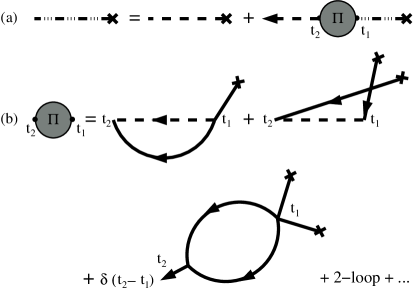
Figure 4: (a) Schwinger-Dyson equation for $\bar{P}(t)$. (b) Perturbative expansion of the polarization operator $\Pi$.

The expansion of $\Pi(t,t_{1})$ in terms of Feynman diagrams is shown in Fig. 4(b). From the Feynman diagrams in Fig. 1, it follows that the number of dotted lines in any given diagram is conserved as one moves from the right to the left. Any diagram contributing to the polarization operator has a single dotted line threading through it from right to left. Also, the only vertex that contributes a factor $Q$ is the $\rm{PPN}$ vertex. Therefore, the $Q$-dependent part of a given diagram has the form $Q^{\#\mbox{of PPN vertices}}\prod_{i}(t_{i}/t_{i+1})^{2Q}$, where the product is over all vertices involving the $P$-line. For a $k$-loop diagram, we can have utmost $2k$ vertices of the type $\rm{PPN}$. Also, it was shown in Ref. KRZ1 that $n$-loop diagrams contribute at the order $\epsilon^{n}$ only. Hence, after coupling constant renormalization, one finds that the expression in square brackets of Eq. (73) is of the form $t^{-2}\sum_{n=1}^{\infty}\epsilon^{n}P_{2n}(Q)$, where $P_{2n}(Q)$ is a polynomial of degree $2n$ in $Q$, and where the factor $t^{-2}$ has been pulled out to give the right dimension.

We can now solve Eq. (73) perturbatively, order by order in $\epsilon$. Simple dimension counting shows that $t^{2Q}\Pi(t,t_{1})t_{1}^{-2Q}=t^{-2}F(t_{1}/t)$, where $F(\tau)$ is a dimensionless function. The previous argument shows that $F(\tau)=\sum_{n=1}^{\infty}\epsilon^{n}P_{2n}(Q)$. Assume a power law solution for $\eta$, i.e., $\eta=ct^{-\theta_{p}}$ where $\theta_{p}=\sum_{n=1}a_{n}\epsilon^{n}$ and $c$ is a constant. Then Eq. (73) simplifies to

$$\theta_{p}=-\int_{0}^{1}d\tau F(\tau)\tau^{-\theta_{p}}.$$ (74)

Expanding $F(\tau)$ and $\theta_{p}$ as series in $\epsilon$, we obtain

$$\sum_{n=1}^{\infty}a_{n}\epsilon^{n}=-\int_{0}^{1}d\tau\sum_{n_{1}=1}^{\infty}P_{2n_{1}}\epsilon^{n_{1}}\sum_{n_{2}=0}^{\infty}\frac{\left[-\theta_{p}\ln(\tau)\right]^{n_{2}}}{n_{2}!}.$$ (75)

Solving Eq. (75) order by order for $a_{n}$, it is easy to verify that the coefficient of $\epsilon^{n}$ is a polynomial of degree $2n$ in $Q$, i.e.,

$$\theta=\sum_{n=0}^{\infty}\epsilon^{n}\left(\sum_{p=0}^{2n}C_{n,p}Q^{p}\right),$$ (76)

where $C_{n,p}$’s are some unknown constants.

Given Eq. (76), it is easy to rederive the one loop correction to $\theta$ (Eq. (47)) obtained by the renormalization group formalism. The three unknowns in the coefficient of $\epsilon$ in Eq. (76) are obtained from the exact results in Eq. (24) giving $C_{1,0}=0$, $C_{1,1}=-3/2$, and $C_{1,2}=1$.

V.2 Two-loop formula for $\zeta(Q)$.

As the mean field answer for the exponent $\zeta$ is $0$, it is desirable to evaluate order $\epsilon^{2}$ correction to Eq. (49). This requires the knowledge of order $\epsilon^{2}$ term in $\theta$.

From Sec. V.1, we know that the term in $\epsilon^{2}$ is a polynomial of degree $4$ in $Q$, i.e.,

$$\theta=dQ+Q(Q-\frac{1}{2})\epsilon+\left(\sum_{k=0}^{4}C_{2,k}Q^{k}\right)\epsilon^{2}+O(\epsilon^{3}).$$ (77)

Out of the $5$ unknown $C_{2,k}$’s, two are fixed by the conditions that $\theta=0$ for $Q=0$ and $\theta=d/2$ for $Q=1/2$ (see Eq. (24). For $Q=1$, it is known that $\theta=d+\epsilon/2+O(\epsilon^{2})$ KRZ1 . We assume that the order $\epsilon^{2}$ term is absent when $Q=1$ (see Appendix for a heuristic validation of this assumption). This fixes the third constant and we are left with

$$\theta=dQ+Q(Q-\frac{1}{2})\epsilon+Q(Q-\frac{1}{2})(Q-1)(AQ+B)\epsilon^{2}+O(\epsilon^{3}),$$ (78)

where $A$ and $B$ are constants.

The constant $A$ is not difficult to calculate. The contribution to $\theta$ of order $\epsilon^{2}Q^{4}$ comes from the square of 1-loop polarization operator and from two-loop diagrams with four $PPN$-vertices. There are only two such diagrams, which are shown in Fig. 5. The numerical computation of corresponding Feynman integrals gives

$$A=(\frac{\pi^{2}}{3}-3)-0.296\ldots\approx-0.006,$$ (79)

where the first term on the right hand side comes from the order-$\epsilon^{2}$ term in the one-loop polarization operator.

Figure 5: The two-loop diagrams contributing to the constant $A$ in Eq. (78).

The calculation of constant $B$ seems an almost impossible task, as there are over twenty two-loop diagrams contributing to it. However, the terms proportional to B drop out of the the two loop expression for $\zeta$. Substituting Eq. (78) into Eq. (3) one finds that

$$\zeta=(2Q-1)\epsilon+(2Q-1)(Q-1)(\frac{1}{2}+AQ)\epsilon^{2}+O(\epsilon^{3}).$$ (80)

In Table 3, we compare the one-loop expression for $\zeta$ (Eq. (49)) and two-loop expression for $\zeta$ (Eq. (80)) with numerical results in $1$-dimension.

Table 3: Comparison of one-loop (Eq. (49)) and two-loop (Eq. (80)) results for $\zeta$ with numerical simulations in $1$-dimension.

$q$	Numerical	$1$-loop	$2$-loop
2	0.00	0.00	0.00
3	$0.21\pm 0.11$	0.33	0.28
4	$0.32\pm 0.08$	0.50	0.44
5	$0.44\pm 0.08$	0.60	0.54
8	$0.59\pm 0.07$	0.75	0.70
16	$0.73\pm 0.06$	0.88	0.85
$\infty$	1.00	1.00	1.00

VI Summary and conclusions

In summary, we develop a systematic method to calculate the persistence exponent $\theta$ for a system of coagulating and annihilating random walkers, in arbitrary dimensions. In $1$-dimension, this corresponds to persistence probabilities of domain walls in the Potts model evolving via zero temperature Glauber dynamics. We establish an exponent relation by which the number of unknown exponents in the problem is reduced from two to one. The unknown persistence exponent $\theta$ is determined perturbatively using the formalism of renormalization group.

The persistence problem studied in this paper can be considered as a special case of a more general problem of the survival probability of a test particle with diffusion constant $\kappa$ times the diffusion constant of the other particles. In this case it is known that the persistence exponent $\theta_{\kappa}(q)$ depends on $\kappa$ monthus ; MC . While simple limiting cases have been studied monthus ; FG ; KNR ; howard via numerics, mean-field or perturbative techniques, a general understanding is still lacking. It would be interesting to extend the formalism of perturbative renormalization group to calculate $\theta_{\kappa}(q)$.

Appendix A Mass distribution in the $A_{i}+A_{j}\rightarrow A_{i+j}$ model

In this appendix, we present a heuristic derivation of the distribution of small masses in the $A_{i}+A_{j}\rightarrow A_{i+j}$ model. This model corresponds to the $Q=1$ limit of the model discussed in the paper. For the $A_{i}+A_{j}\rightarrow A_{i+j}$ model, it is known spouge ; KRZ1 that for $m\ll t^{d/2}$,

$$\bar{P}(m,t)\sim\cases{\frac{m}{t^{3/2}}&in $d=1$,\cr\frac{m^{(\epsilon+O(\epsilon^{2}))/d}}{t^{d+\epsilon/2+O(\epsilon^{2})}}&in $1\leq d<2$,\cr\frac{\ln(m)\ln(t)}{t^{2}}&in $d=2$,\cr\frac{1}{t^{2}}&in $d>2$.\cr}$$ (81)

In this appendix, we give a heuristic argument as to why the terms of order $\epsilon^{2}$ and higher could be absent, as a result of which the expansion up to order $\epsilon$ gives the exact answer.

Putting $\lambda_{a}=0$ in Eq. (8), we obtain that the mass distribution $P(m,x,t)$ evolves according to

$$\left(\frac{\partial}{\partial t}-D\nabla^{2}\right)P=\lambda_{c}P*P-2\lambda_{c}NP+i\sqrt{2\lambda_{c}}\xi P,$$ (82)

where $N=\int_{0}^{\infty}dmP(m)$ is the density of particles and $P*P=\int_{0}^{m}dm^{\prime}P(m^{\prime})P(m-m^{\prime})$. The density obeys the equation:

$$\left(\frac{\partial}{\partial t}-D\nabla^{2}\right)N=\lambda_{c}N^{2}+i\sqrt{2\lambda_{c}}\xi N.$$ (83)

Let

$$F(s,t)=\int_{0}^{\infty}dmP(m,t)e^{-ms}$$ (84)

be the Laplace transform of $P(m,t)$. Then,

$$B(s,t)=N(t)-F(s,t),$$ (85)

obeys the equation

$$\left(\frac{\partial}{\partial t}-D\nabla^{2}\right)B=\lambda_{c}B^{2}+i\sqrt{2\lambda_{c}}\xi B.$$ (86)

The function $B(s,t)$ obeys the same equation as the density $N$ oleg . However, the initial conditions at $t=0$ are different. If the initial density of particles $N(0)=N_{0}$, then $B(s,0)=N_{0}(1-e^{-s})$. Therefore, if the average particle density is $\bar{N}(N_{0},t)$, then

$$\bar{F}(s,t)=\bar{N}(N_{0},t)-\bar{N}(N_{0}(1-e^{-s}),t).$$ (87)

The function $F(s,t)$ will have the scaling form

$$\bar{F}(s,t)\sim\frac{1}{t^{d/2}}g(st^{d/2}),$$ (88)

where the scaling function $g(x)\sim x^{-\phi}$ for $x\gg 1$. On performing the inverse Laplace transform, we obtain

$$\bar{P}(m,t)\sim\frac{m^{\phi-1}}{t^{d/2(1+\phi)}}.$$ (89)

Thus, if $\phi$ were equal to $2/d$, the expression in Eq. (81) to is exact order $\epsilon$.

To calculate $\phi$, we look at the behavior of the particle density $\bar{N}$. It is expected to have the scaling form

$$\bar{N}=N_{0}h(N_{0}t^{d/2})$$ (90)

where the scaling function $h(x)$ behaves for large $x$ as

$$h(x)\sim\frac{1}{x}(1+\frac{1}{x^{\psi}}),\qquad x\gg 1,$$ (91)

where $\psi$ is some exponent greater than zero.

Substituting Eqs. (90) and (91) into Eq. (87), it is straightforward to verify that

$$\phi=\psi.$$ (92)

In $1$- and $2$-dimensions, it is easy enough to verify that $\psi=2$ and $\psi=1$ respectively, consistent with the exact results in Eq. (81). In other dimensions, we argue as follows. The density of particles in the $A_{i}+A_{j}\rightarrow A_{i+j}$ model is inversely proportional to the area swept out by a random walker in time $t$. This area varies as $(\sqrt{t+c})^{d}$, where $c$ is some constant. Then, the particle density decays as $\bar{N}\sim t^{-d/2}(1-\rm{const}/t)$, such that

$$\psi=\frac{2}{d}.$$ (93)

Substituting into Eq. (89), we obtain

$$\bar{P}(m,t)\sim\frac{m^{(2-d)/d}}{t^{d/2+1}}.$$ (94)

which is the one-loop answer in Eq. (81).

References

- (1) S. N. Majumdar, Curr. Sci. (India) 77, 370 (1999).
- (2) J. Cardy, J. Phys. A 28 L19 (1995).
- (3) S. N. Majumdar and S. J. Cornell, Phys. Rev. E. 57, 3757 (1998).
- (4) M. Donsker and S. R. S. Varadhan, Commun. Pure Appl. Math. 28, 525 (1975).
- (5) V. Mehra and P. Grassberger, Phys. Rev. E. 65, 0501101 (2001).
- (6) S. J. O’Donoghue and A. J. Bray, Phys. Rev. E 65, 051113 (2002).
- (7) R. A. Blythe and A. J. Bray, J. Phys. A 35, 10503 (2002).
- (8) E. K. O. Hellén and M. J. Alava, Phys. Rev. E 66, 026120 (2002).
- (9) E. K. O. Hellén, P. E. Salmi and M. J. Alava, Europhys. Lett. 59, 186 (2002).
- (10) S. Krishnamurthy, R. Rajesh, and O. Zaboronski, Phys. Rev. E 66, 066118 (2002).
- (11) S. Redner and P. L. Krapivsky, Am.J. Phys. 67, 1277.
- (12) J. Cardy and M. Katori, J. Phys. A 36, 609 (2003).
- (13) B. Derrida, V. Hakim and V. Pasquier, Phys. Rev. Lett. 75, 751 (1995).
- (14) C. Monthus, Phys. Rev. E. 54, 4844 (1996).
- (15) S. J. O’Donoghue and A. J. Bray, Phys. Rev. E 65, 051114 (2002).
- (16) E. Ben-Naim and P. L. Krapivsky, Phys. Rev. E. 56, 3788 (1997).
- (17) B. Derrida J. Phys. A 28, 1481 (1995).
- (18) S. N. Majumdar and D. Huse, Phys. Rev. E 52, 270 (1995).
- (19) C. Sire and S. N. Majumdar, Phys. Rev. Lett. 74, 4321 (1995); Phys. Rev. E 52, 244 (1995).
- (20) L. Peliti, J. Phys. A 19, L365 (1986).
- (21) D. Toussaint and F. Wilczek, J. Chem. Phys. 78, 2642, 1983; D. C. Torney and H. M. McConnell, J. Phys. Chem 87, 1941 (1983); A. A. Lushnikov, Phys. Lett. 120 135 (1987); B. P. Lee, J. Phys. A 27, 2633 (1994); J. G. Amar and F. Family, Phys. Rev. A 41, 3258 (1990).
- (22) J. L. Spouge, Phys. Rev. Lett. 60, 871 (1988).
- (23) M. Bramson and D. Griffeath, Ann. of Prob. 8, 183 (1980).
- (24) K. Kang and S. Redner, Phys. Rev. A 30, 2833 (1984).
- (25) O. Zaboronski, Phys. Letts. A 281, 119 (2001).
- (26) M. Doi, J. Phys. A 9, 1465 (1976); M. Doi, J. Phys. A 9, 1479 (1976); Ya. B. Zel’dovich and A. A. Ovchinnikov, Soviet Phys. JETP 47, 829 (1978).
- (27) J. Cardy, Field theory and nonequilibrium statistical mechanics. The notes can be obtained at the website http://www-thphys.physics.ox.ac.uk/users/JohnCardy/
- (28) D. C. Mattis and M. L. Glasser, Rev. Mod. Phys. 70, 979 (1998).
- (29) B. P. Lee, J. Phys. A 27, 2633 (1994).
- (30) B. Derrida and R. Zeitak, Phys. Rev. E. 54, 2513 (1996).
- (31) T. Masser and D. ben-Avraham, Phys. Lett. A. 275, 382 (2000).
- (32) E. Ben-Naim, L. Frachebourg and P. L. Krapivsky, Phys. Rev. E 53, 3078(1996).
- (33) C. Itzykson and J.-M. Drouffe, Statistical Field Theory, Cambridge monographs on mathematical physics, Cambridge University Press (1994).
- (34) The effective reaction rate entering the Smoluchowski coagulation equation is not equal to the bare reaction rate. This is due to strong ultraviolet divergence of Feynman integrals contributing to renormalization of the reaction rate. As a result, the density-density correlation function is not equal to the product of one-point functions, but rather is proportional to it. Yet, as the renormalized reaction rate in is a constant depending on lattice spacing, decay exponents are predicted by the mean field correctly.
- (35) M. E. Fisher and M. P. Gelfand, J. Stat. Phys. 53, 175 (1988).
- (36) P. L. Krapivsky, E. Ben-Naim and S. Redner, Phys. Rev. E. 50, 2474 (1994).
- (37) M. J. Howard, J. Phys. A. 29, 3437 (1996).