Magnetic Interactions in Transition-Metal Oxides

Abstract

The correct understanding of the nature and dynamics of interatomic magnetic interactions in solids is fundamentally important. In addition to that it allows to address and solve many practical questions such as stability of equilibrium magnetic structures, designing of magnetic phase diagrams, the low-temperature spin dynamics, etc. The magnetic transition temperature is also related with the behavior of interatomic magnetic interactions. One of the most interesting classes of magnetic compounds, which exhibits the rich variety of the above-mentioned properties in the transition-metal oxides. There is no doubts that all these properties are related with details of the electronic structure. In the spin-density-functional theory (SDFT), underlying many modern first-principles electronic structure methods, there is a certain number of fundamental theorems, which in principles provides a solid theoretical basis for the analysis of the interatomic magnetic interactions. One of them is the magnetic force theorem, which connects the total energy change with the change of single-particle energies obtained from solution of the Kohn-Sham equations for the ground state. The basic problem is that in practical implementations SDFT is always supplemented with additional approximations, such as local-spin-density approximation (LSDA), LSDA + Hubbard $U$, etc., which are not always adequate for the transition-metal oxides. Therefore, there is not perfect methods, and the electronic structure we typically have to deal with is always approximate. The main purpose of this article, is to show how this, sometimes very limited information about the electronic structure extracted from the conventional calculations can be used for the solution of several practical questions, accumulated in the field of magnetism of the transition-metal oxides. This point will be illustrated for colossal-magnetoresistive manganites, double perovskites, and magnetic pyrochlores. We will review both successes and traps existing in the first-principle electronic structure calculations, and make connections with the models which capture the basic physics of the considered compounds. Particularly, we will show what kind of problems can be solved by adding the Hubbard $U$ term on the top of the LSDA description. It is by no means a panacea from all existing problems of LSDA, and one should clearly distinguish the cases when $U$ is indeed indispensable, play a minor role, or may even lead to the systematic error.

1 Introduction

The first-principles electronic structure calculations play a very important role in the exploration of magnetism. They have been successfully applied for various types of metallic compounds. The transition-metal oxides (TMO), however, take a very special place in this classification and typically regarded as a counter-example where the first-principles calculations either experience serious difficulties or simply do not work. Such an extreme point of view has of course a very serious background because most of modern computational techniques are based on the spin-density-functional theory (SDFT), designed for the ground state, which is typically supplemented with the local-spin density approximation (LSDA) for the exchange-correlation interactions. The latter is based on the homogeneous electron gas theory, and therefore is very different from the localized-orbital limit, which was originally adopted for the description of TMO [1, 2, 3, 4].

Therefore, traditionally there was a big gap in the understanding of interatomic magnetic interactions in TMO basing on these model arguments and the first-principles electronic structure calculations [5, 6], which appeared only in the middle of 1980s and were regarded as very challenging at that time.

Since then, two different standpoints have certainly became closer. It is true that due to complexity of the problem of exchange and correlations, even now there is no perfect computational methods for the transition-metal oxides. However, it also becomes increasingly clear that the model analysis of the problem should use results of first-principles electronic structure calculations, at least as a starting point. In many cases, a puzzling behavior attributed to the fanciful correlation effects can be naturally explained by details of the realistic electronic structure.

The purpose of this article is to make a link between general formulation of SDFT and models of interatomic magnetic interactions for TMO. We will try to show that even in the present form the electronic structure calculations can play a very important role in the understanding of magnetic properties of various TMO, despite many limitations inherent to LSDA and some of its refinements.

In Sec. 2 we will summarize main results of SDFT and formulate the magnetic force theorem which presents the basis for the analysis of magnetic interactions in solids. The connection of this theorem with some canonical models for interatomic magnetic interactions will be illustrated in Sec. 3. In Sec. 4 we will present a critical analysis of interatomic magnetic interactions in MnO basing on several available methods of electronic structure calculations. In Sec. 5 we will consider some practical problems related with the colossal-magnetoresistive (CMR) manganites, double perovskites Sr₂Fe$M$O₆ ($M$$=$ Mo and Re), and magnetic pyrochlores $A_{2}$Mo₂O₇ ($A$$=$ Y, Gd, and Nd).

The insulating character of many TMO presents one of the most interesting and controversial problems. Particularly, it is well known that LSDA frequently underestimates or even fails to reproduce the energy gap, which is formally the excited state property. Is it possible that even in this case, it can provide a physically meaningful description for the parameters of the ground state, such as the interatomic magnetic interactions? In this context, we will consider the role played by the on-site Coulomb interaction $U$ on the top of the LSDA electronic structure and argue that one should clearly distinguish the behavior of band insulators, which is governed by the double exchange (DE) physics [2, 7], and in principle can be accounted for by itinerant models, in the spirit of LSDA, from the behavior of Mott insulators, where the Coulomb $U$ is indeed indispensable in order to suppress (in this case) spurious DE interactions and unveil the completely different physical behavior governed by the superexchange (SE) interactions [3, 4, 8]. A brief summary and perspectives will be outlined in Sec. 6.

2 Theory of magnetic interactions in solids

2.1 Spin-Density-Functional Theory

The modern way to approach the problem of interatomic magnetic interactions in solids is based on the SDFT [9], which states that the magnetic ground state of the $N$-electron system can be obtained by minimizing the Hohenberg-Kohn total energy functional

$$E[{\bf m}]=T_{0}[{\bf m}]+E_{\rm XC}[{\bf m}]$$ (1)

($T_{0}[{\bf m}]$ being the kinetic energy of a non-interaction electron system and $E_{\rm XC}[{\bf m}]$ being the exchange-correlation energy) with respect to the spin-magnetization density ${\bf m}({\bf r})$.

The direct implementation of the SDFT is hampered by the fact that the functional dependencies $T_{0}[{\bf m}]$ and $E_{\rm XC}[{\bf m}]$ are generally unknown. In the case of $T_{0}[{\bf m}]$, the problem is resolved by introducing an auxiliary system of one-electron orbitals $\{\psi_{i}({\bf r})\}$, and requesting the kinetic energy (in Rydberg units),

$$T_{0}[{\bf m}]=\sum_{i=1}^{N}\int d{\bf r}\psi_{i}^{\dagger}({\bf r})\left(-\nabla^{2}\right)\psi_{i}({\bf r}),$$

the spin-magnetization density,

$${\bf m}({\bf r})=\sum_{i=1}^{N}\psi_{i}^{\dagger}({\bf r})\bm{\sigma}\psi_{i}({\bf r})$$ (2)

($\bm{\sigma}$ being the vector of Pauli matrices), and the total energy to coincide with the same parameters of the real many-electron system in the ground state. Then, the minimization of $E[{\bf m}]$ with respect to ${\bf m}({\bf r})$ is equivalent to the self-consistent solution of single-particle Kohn-Sham (KS) equations for $\{\psi_{i}({\bf r})\}$:

$$\left[-\nabla^{2}+\bm{\sigma}\cdot{\bf B}({\bf r})\right]\psi_{i}({\bf r})=\varepsilon_{i}\psi_{i}({\bf r}),$$ (3)

where the effective magnetic field is given by

$${\bf B}({\bf r})=\frac{\delta}{\delta{\bf m}({\bf r})}E_{\rm XC}[{\bf m}].$$

The exchange-correlation energy functional, $E_{\rm XC}[{\bf m}]$, is typically taken in an approximate form. Several possible approximations along this line are listed below.

• The local-spin-density approximation. In this case, the explicit dependence of $E_{\rm XC}$ on ${\bf m}({\bf r})$ and the electron density $n({\bf r})$,

  $$E_{\rm XC}[n,{\bf m}]=\int d{\bf r}n({\bf r})\varepsilon_{\rm XC}\left[n({\bf r}),|{\bf m}({\bf r})|\right],$$ (4)

  is borrowed from the theory of homogeneous electron gas. Conceptually, LSDA is similar to the Stoner theory of band magnetism [10]. Due to the rotational invariance of the homogeneous electron gas, $E_{\rm XC}$ depends only on the absolute value of ${\bf m}({\bf r})$.

• The local-density approximation plus Hubbard $U$ (LDA$+$$U$) approach [11, 12, 13]. This is a semi-empirical approach, the main idea of which is to cure some shortcomings of the LSDA description for the localized electron states by replacing corresponding part of $E_{\rm XC}[n,{\bf m}]$ in LSDA by the energy of on-site Coulomb interactions, in an analogy with the multi-orbital Hubbard model. The latter is typically taken in the mean-field Hartree-Fock form:

  $$E_{\rm XC}[\widehat{n}^{\bm{\tau}}]=\sum_{\{\gamma\}}\left(U_{\gamma_{1}\gamma_{3}\gamma_{2}\gamma_{4}}-U_{\gamma_{1}\gamma_{3}\gamma_{4}\gamma_{2}}\right)n_{\gamma_{1}\gamma_{2}}^{\bm{\tau}}n_{\gamma_{3}\gamma_{4}}^{\bm{\tau}},$$

  where $U_{\gamma_{1}\gamma_{3}\gamma_{2}\gamma_{4}}$$\equiv$$\langle\gamma_{1}\gamma_{3}|\frac{1}{r_{12}}|\gamma_{2}\gamma_{4}\rangle$ are the matrix elements of the on-site Coulomb interactions, which are assumed to be renormalized from the bare atomic values by interactions with other (itinerant) electrons and by correlation effects in solids. The electron and spin-magnetization densities for the localized states are represented by corresponding elements of the density matrix $\widehat{n}^{\bm{\tau}}$$=$$\|n_{\gamma_{1}\gamma_{2}}^{\bm{\tau}}\|$ in the basis of atomic-like orbitals $\{\gamma\}$ at the site ${\bm{\tau}}$. Because of this construction, the LDA$+$$U$ approach is basis-dependent and typically implemented in the linear muffin-tin orbital method [14].

• The optimized effective potential (OEP) method [15, 16] is an attempt of exact numerical solution of the KS problem, which does not rely on the local-spin-density approximation for $E_{\rm XC}[n,{\bf m}]$. In this case, the eigenfunctions $\{\psi_{i}({\bf r})\}$ and eigenvalues $\{\varepsilon_{i}\}$ obtained from the KS equations (3) with some trial potential are used as an input for total energy calculations beyond the homogeneous electron gas limit. The parameters of such potential are requested to minimize the total energy.

2.2 Magnetic Force Theorem

The basic idea behind analysis of interatomic magnetic interactions in solids is to evaluate the total energy change $\Delta E$$=$$E[\widehat{R}_{\bm{\theta}}{\bf e}_{\rm GS}]$$-$$E[{\bf e}_{\rm GS}]$ caused by small non-uniform rotations of the spin-magnetization density near the ground state, where ${\bf e}_{\rm GS}({\bf r})$$=$${\bf m}_{\rm GS}({\bf r})/|{\bf m}_{\rm GS}({\bf r})|$ is the direction of the spin-magnetization in the ground state and $\widehat{R}_{\bm{\theta}}$ is the three-dimensional rotation by the (small) angle $\bm{\theta}({\bf r})$, which depends on the position ${\bf r}$ in the real space:

$$\widehat{R}_{\bm{\theta}({\bf r})}{\bf e}_{\rm GS}({\bf r})={\bf e}_{\rm GS}({\bf r})+[\bm{\theta}({\bf r})\times{\bf e}_{\rm GS}({\bf r})]-\frac{1}{2}\bm{\theta}^{2}({\bf r}){\bf e}_{\rm GS}({\bf r}).$$

Thus, characterizes the local stability of the magnetic ground state with respect to non-uniform rotations of the spin-magnetization density.

Very generally, the problem can be solved by minimizing the constrained total energy functional:

$$E_{\bf h}[{\bf m}]=T_{0}[{\bf m}]+E_{\rm XC}[{\bf m}]-\int d{\bf r}{\bf h}({\bf r})\cdot\left[{\bf e}({\bf r})-\widehat{R}_{\bm{\theta}({\bf r})}{\bf e}_{\rm GS}({\bf r})\right],$$

where the constraining field ${\bf h}({\bf r})$ plays the role of Lagrange multipliers and enforces the requested distribution of the spin-magnetization density in the real space.

The magnetic force theorem states in this respect: in the second order of $\bm{\theta}({\bf r})$ the total energy change is solely determined by the change of the KS single-particle energies [18],

$$\Delta E=\sum_{i=1}^{N}\left(\varepsilon_{i}\left[\widehat{R}_{\bm{\theta}}{\bf B},\widehat{R}_{\bm{\theta}}{\bf m}_{\rm GS}\right]-\varepsilon_{i}\left[{\bf B},{\bf m}_{\rm GS}\right]\right)+O\left(\bm{\theta}^{2}\right).$$ (5)

The eigenvalues $\varepsilon_{i}\left[\widehat{R}_{\bm{\theta}}{\bf B},\widehat{R}_{\bm{\theta}}{\bf m}_{\rm GS}\right]$, corresponding to the rotated effective field $\widehat{R}_{\bm{\theta}}{\bf B}$ and the ground state spin-magnetization density $\widehat{R}_{\bm{\theta}}{\bf m}_{\rm GS}$, can be expressed in terms of expectation values of the KS Hamiltonian,

$$\varepsilon_{i}\left[\widehat{R}_{\bm{\theta}}{\bf B},\widehat{R}_{\bm{\theta}}{\bf m}_{\rm GS}\right]=\int d{\bf r}\psi_{i}^{\dagger}[\widehat{R}_{\bm{\theta}}{\bf m}_{\rm GS}]\left(-\nabla^{2}+\bm{\sigma}\cdot\widehat{R}_{\bm{\theta}}{\bf B}\right)\psi_{i}[\widehat{R}_{\bm{\theta}}{\bf m}_{\rm GS}],$$

with $\{\psi_{i}[\widehat{R}_{\bm{\theta}}{\bf m}_{\rm GS}]\}$ yielding $\widehat{R}_{\bm{\theta}}{\bf m}_{\rm GS}$ after substitution into Eq. (2).

The theorem can be reformulated in a different way: the effect of the longitudinal change of ${\bf m}({\bf r})$ on $T_{0}[{\bf m}]$ and $E_{\rm XC}[{\bf m}]$ caused by the self-consistent solution of the KS equations (3) with the external magnetic field ${\bf h}({\bf r})$ is cancelled out in the second order of $\bm{\theta}({\bf r})$.

The theorem can be proven rather generally provided that the exchange-correlation energy functional obeys the following condition [18]:

$$E_{\rm XC}[{\bf m}]=E_{\rm XC}[\widehat{R}_{\bm{\theta}}{\bf m}].$$ (6)

In LSDA, it immediately follows from Eq. (4). More generally, Eq. (6) can be regarded as the fundamental gauge-symmetry constraint, which should be superimposed on the admissible form of the exchange-correlation energy functionals [19].

The magnetic force theorem has very important consequences:

• Generally, the KS eigenvalues $\{\varepsilon_{i}\}$ have no physical meaning and cannot be compared with the true single-particle excitations (that is typically the case for many spectroscopic applications). In this respect, the magnetic excitations present a pleasant exception, thanks to the magnetic force theorem.

• In principle, the knowledge of the effective KS potential alone is sufficient to calculate the total energy difference. It allows to get rid of heavy total energy calculations (particularly, for the OEP method) without any loss of the accuracy.

2.3 Practical Implementations of the Magnetic Force Theorem

In most cases, practical applications of the magnetic force theorem are based on relaxed constraint conditions in comparison with the ones given by Eq. (5). Namely, the second condition requesting the KS eigenvalues to correspond the rotated spin magnetization density is typically dropped and $\varepsilon_{i}\left[\widehat{R}_{\bm{\theta}}{\bf B},\widehat{R}_{\bm{\theta}}{\bf m}_{\rm GS}\right]$ is replaced by $\varepsilon_{i}\left[\widehat{R}_{\bm{\theta}}{\bf B}\right]$ obtained from the KS equations (3) with the rotated field $\widehat{R}_{\bm{\theta}}{\bf B}$. This considerably facilitates the calculations, though at the cost of a systematic error, which was recently discussed by Bruno [20]. We will return to this problem in Sec. 5.1.4 where will give some estimates of this error and discuss some physical implications which may be related with the additional rotation of the spin-magnetization density for the transition-metal oxides. In this section we will review some practical schemes of calculations, which ignore these effects. Basically, they are two.

The first one is based on the perturbation theory expansion for the Green function [21]

$$G({\bf r},{\bf r}^{\prime},\varepsilon)=\sum_{i}\frac{\psi_{i}({\bf r})\psi_{i}^{\dagger}({\bf r}^{\prime})}{\varepsilon-\varepsilon_{i}+i\delta}$$

and its projections

$$G^{\uparrow,\downarrow}=\frac{1}{2}{\rm Tr}_{S}\left\{(1\mp\sigma_{z})G\right\}$$

on the majority ($\uparrow$) and minority ($\downarrow$) spin states (${\rm Tr}_{S}$ being the trace over the spin indices). In the second order of $\bm{\theta}({\bf r})$, the total energy change can be mapped onto the Heisenberg model

$$\Delta E=-\frac{1}{2}\int d{\bf r}\int d{\bf r}^{\prime}J({\bf r},{\bf r}^{\prime})\left[\widehat{R}_{\bm{\theta}({\bf r})}{\bf e}_{\rm GS}({\bf r})\cdot\widehat{R}_{\bm{\theta}({\bf r}^{\prime})}{\bf e}_{\rm GS}({\bf r}^{\prime})-{\bf e}_{\rm GS}({\bf r})\cdot{\bf e}_{\rm GS}({\bf r}^{\prime})\right].$$ (7)

The parameters of this model are given by [21]

$$J({\bf r},{\bf r}^{\prime})=\frac{2}{\pi}{\rm Im}\int_{-\infty}^{\varepsilon_{F}}d\varepsilon G^{\uparrow}({\bf r},{\bf r}^{\prime},\varepsilon)B({\bf r}^{\prime})G^{\downarrow}({\bf r}^{\prime},{\bf r},\varepsilon)B({\bf r}),$$ (8)

where $\varepsilon_{F}$ is the Fermi energy corresponding to the highest occupied KS orbital. All practical calculations along this line are typically performed on a discrete lattice, assuming that all space is divided into atomic regions specified by the site indices $\{\bm{\tau}\}$, so that the angles $\bm{\theta}({\bf r})$ depend only on $\bm{\tau}$, and neglecting the effects caused by rotations of the spin-magnetization density on the intra-atomic scale. In the discrete version, $G^{\uparrow,\downarrow}({\bf r},{\bf r}^{\prime},\varepsilon)$ is expanded in the basis of atomic-like orbitals $\{\gamma\}$ centered at different atomic sites (for example, in the nearly-orthogonal LMTO representation [14]). The integral over atomic regions around $\bm{\tau}$ and $\bm{\tau}^{\prime}$, $J_{\bm{\tau}\bm{\tau}^{\prime}}$$=$$\int_{\bm{\tau}}d{\bf r}\int_{\bm{\tau}^{\prime}}d{\bf r}^{\prime}J({\bf r},{\bf r}^{\prime})$, defines conventional parameters of interatomic magnetic interactions in the real space.

The main idea of the second approach is to calculate the energy of the collective spin excitation corresponding to the frozen spin wave with the vector ${\bf q}$. The method, which is called the frozen (or adiabatic) spin-wave approximation is designed for the discrete lattice [23]. In this context, the adiabaticity means that the directions of the spin-magnetization can be regarded as the ”slow” variables, so that for each configuration specified by $\widehat{R}_{\bm{\theta}}$ the ”fast” electronic degrees of freedom have enough time to follow this directional distribution of the spin-magnetization density. The rotation matrix $\widehat{R}_{\bm{\theta}}$ is requested to transform the collinear distribution of the spin magnetic moments in the ground state, ${\bf m}_{\bm{\tau}}$$=$$\int_{\bm{\tau}}d{\bf r}~{}{\bf m}_{\rm GS}({\bf r})$, to the spin spiral: ${\bf m}_{\bm{\tau}}$$\rightarrow$$(\cos{\bf q}\cdot\bm{\tau}\sin\theta_{\bm{\tau}},\sin{\bf q}\cdot\bm{\tau}\sin\theta_{\bm{\tau}},\cos\theta_{\bm{\tau}})|{\bf m}_{\bm{\tau}}|$. If ${\bf m}_{\bm{\tau}}$$||$$z$, the rotation angles are given by

$$\bm{\theta}_{\bm{\tau}}=\left(-\sin{\bf q}\cdot\bm{\tau},\cos{\bf q}\cdot\bm{\tau},0\right)\theta_{\bm{\tau}}$$

($\theta_{\bm{\tau}}$ being the cone-angle of the spin wave). The KS equations for the spin-spiral configuration of the effective field $\widehat{R}_{\bm{\theta}}{\bf B}$ can be solved by employing the generalized Bloch transformation [24]. This gives the total energy change $\Delta E({\bf q},\bm{\theta})$ corresponding to the ”excited” spin-spiral configuration with the vector ${\bf q}$. In the the second order of $\bm{\theta}$, this energy change can be mapped onto the Heisenberg model. The mapping provides parameters of magnetic interactions in the reciprocal space, $J_{\bf q}$, which can be Fourier transformed to the real space.

3 Relation with the Models of Magnetic Interactions

The application of Eq. (8) goes far beyond the standard electronic structure calculations. It is rather general, and many canonical expressions for magnetic interactions in solids can be derived starting with Eq. (8). Here we would like to illustrate this idea by considering two model examples.

3.1 Double Exchange and Superexchange Interactions in Half-Metallic Ferromagnetic State

Consider the ferromagnetic (FM) chain of atoms, described by the Hamiltonian

$${\cal H}_{\tau\tau^{\prime}}=-t_{0}\delta_{\tau\pm 1,\tau^{\prime}}+\sigma_{z}B,$$

which is an analog of the KS Hamiltonian (3) on the discrete lattice, where matrix elements of the kinetic energy $t_{0}$ (the transfer integrals) are restricted by the nearest neighbors, and $B$ is the effective field polarizing the conduction electrons parallel to the $z$ axis. The half-metallic behavior implies that $t_{0}$$<$$B$ and the electron density $n$$<$$1$ (which corresponds to the partial population of the $\uparrow$-spin band in Fig. 1).

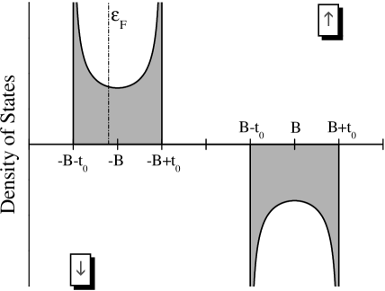
Figure 1: Schematic density of states for the half-metallic ferromagnetic chain.

The problem can be easily solved analytically, and by expanding $G_{\tau\tau^{\prime}}^{\downarrow}(\varepsilon)$ in Eq. (8) up to the second order of $t_{0}/B$ one can obtain the following contributions to the nearest-neighbor (NN) exchange coupling [25]:

$$J^{D}=\frac{t_{0}}{2\pi}\sin\pi n$$ (9)

and

$$J^{S}=-\frac{t_{0}^{2}}{2\pi B}(\pi n+\frac{1}{2}\sin 2\pi n).$$ (10)

$J^{D}$ is the FM double exchange interaction, which is proportional to $t_{0}$. $J^{S}$ is the antiferromagnetic (AFM) superexchange interaction. For the half-filled band at $n$$=$$1$ the system is insulating. Then, $J^{D}$$=$$0$, while Eq. (10) leads to the standard expression for the SE interaction at the half-filling: $J^{S}$$=$$-$$\frac{t_{0}^{2}}{2B}$ [4].

More generally, $J^{D}$ and $J^{S}$ can be expressed through the moments of local density of states, and $J^{D}$ is the measure of the kinetic energy of the fully spin-polarized half-metallic states [26]. Originally, the concept of the double exchange was introduced for the metallic phase of CMR manganites [7]. However, the phenomenon appears to be more generic and one of the most interesting recent suggestions was that the same mechanism can operate in the insulating state, provided that the system is a band insulator [26]. This substantially modifies the original view on the problem and combine two seemingly orthogonal concepts, one of which is the DE physics and the other one is the insulating behavior of some CMR manganites. We will return to this problem in Sec. 5.1.

3.2 Superexchange Interaction via Oxygen States

Consider the interaction between two magnetic (transition-metal) site, which is mediated by the non-magnetic oxygen states (Fig. 2,

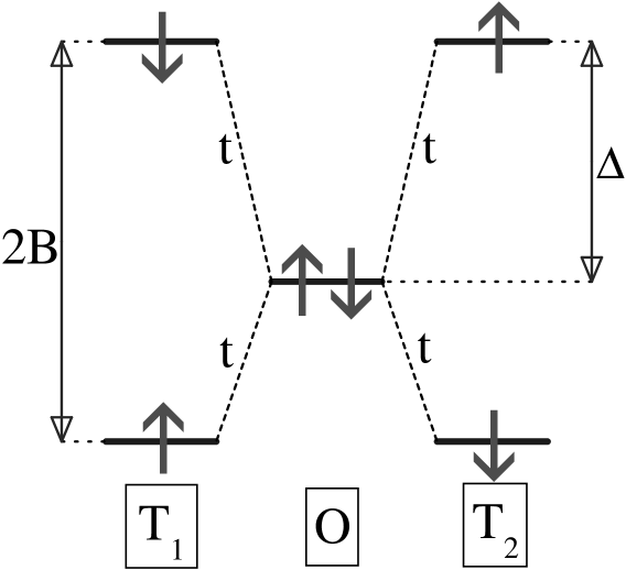
Figure 2: Positions of atomic levels illustrating the superexchange interaction between transition-metal sites mediated by the oxygen states.

the situation is rather common for the insulating transition-metal oxides). It is assumed that the splitting between the $\uparrow$- and $\downarrow$-spin states of the transition metal sites is $2B$. $\Delta$ describes the relative position of the oxygen states relative to the transition-metal states (the so-called charge-transfer energy). It is further assumed that the occupied states are T₁($\uparrow$), T₂($\downarrow$), and O($\uparrow$,$\downarrow$), and the unoccupied states are T₁($\downarrow$) and T₂($\uparrow$). $2B$ and $\Delta$ are the largest parameters in the problem, so that the transfer interactions $t$ between the transition-metal and oxygen sites can be treated as a perturbation starting with the atomic limit. Corresponding matrix elements of the Green function connecting the sites T₁ and T₂ are given by

$$G^{\uparrow}_{12}(\varepsilon)=G^{\downarrow}_{21}(\varepsilon)=t^{2}(\varepsilon+B)^{-1}(\varepsilon-B+\Delta)^{-1}(\varepsilon-B)^{-1}.$$ (11)

Then, using Eq. (8) one can obtain the well-known expression for the SE interactions mediated by the oxygen states [27]:

$$J^{S}_{12}=-\frac{t^{4}}{\Delta^{2}}\left(\frac{1}{\Delta}+\frac{1}{2B}\right),$$

which describes the shift of the poles of the Green function (11) of the occupied states, located at $\varepsilon$$=$$-$$B$ and $\varepsilon$$=$$B$$-$$\Delta$, due to the interaction with the unoccupied states located at $\varepsilon$$=$$B$.

Considered examples of DE and SE interactions show that Eq. (8) is rather universal and can be regarded as the starting point for the general analysis of interatomic magnetic interactions in solids. The applications can be very wide and cover, for example, the theory of RKKY interactions [28], the effects of the interatomic Coulomb interactions on the SE coupling [29], etc.

4 Electronic Structure of MnO from the viewpoint of Interatomic Magnetic Interactions

The manganese monoxide provides an excellent opportunity to test available methods of electronic structure calculations for the transition-metal oxides. While numerous spectroscopic techniques deal mainly with the excited state properties, which cannot be compared directly with results of electronic structure calculations designed for the ground state, the interatomic magnetic interactions are the ground-state properties and, in principle, should be accounted for by these calculations.

The interatomic magnetic interactions in MnO are well studied experimentally. The magnetic behavior of MnO can be described by the simple Heisenberg model including first ($J_{1}$$=$$-$$4.8$ meV) and second ($J_{2}$$=$$-$$5.6$ meV) neighbor interactions [30]. Since MnO is a wide-gap insulator, it is clear that both interactions originate from the superexchange mechanism [4, 5].

One can easily design the proper model for the electronic structure of MnO using the following arguments [18]. Since the electronic configuration of the Mn atoms in MnO is close to $3d^{5}_{\uparrow}3d^{0}_{\downarrow}$, both from the viewpoint of the model valence arguments and the electronic structure calculations, the distribution of the spin-magnetization density near Mn sites is nearly spherical. Therefore, the only parameter of the effective magnetic field at the Mn sites we need to worry about is $B$, which controls the splitting between occupied $3d_{\uparrow}$ and unoccupied $3d_{\downarrow}$ states. Another important parameter of the electronic structure is the charge-transfer energy $\Delta$, which controls the relative position of the $3d_{\downarrow}$ and the oxygen $2p$ states. Then, using an analogy with the model for SE interactions considered in Sec. 3.2, one can try to parameterize the effective KS potential in terms of $B$ and $\Delta$ (basically in the spirit of LDA$+$$U$ for the half-filled $3d$ shell), and to find these two parameters by fitting two experimental parameters of interatomic magnetic interactions, $J_{1}$ and $J_{2}$, provided that the kinetic and non-magnetic parts of the effective KS Hamiltonian are well described on the level of LDA.

The fitting, which is very straightforward in the nearly-orthogonal LMTO basis [14, 18], yields the following parameters: $B$$\simeq$$5.3$ eV and $\Delta$$\simeq$$10.7$ eV. The corresponding density of states is shown in Fig. 3, together with results of the LSDA, LDA$+$$U$, and OEP calculations.

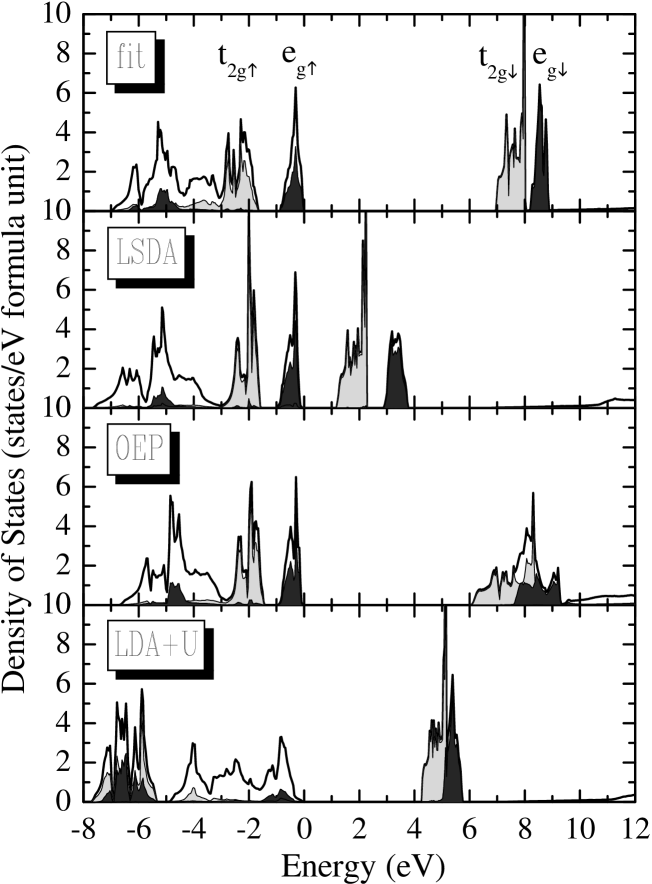
Figure 3: Electronic structure of MnO, which fits the experimental parameters of magnetic interactions together with results of first-principles calculations in LSDA, OEP, and LDA$+$$U$.

Corresponding parameters of magnetic interactions are listed in Table 1.

Table 1: Parameters of magnetic interactions in MnO obtained in LSDA, OEP and LDA$+$$U$ in comparison with experimental data [30].

	$J_{1}$ (meV)	$J_{2}$ (meV)
LSDA	-13.2	-23.5
OEP	-8.9	-12.0
LDA$+U$	-5.0	-13.2
Expt.	-4.8	-5.6

Unfortunately, none of the existing techniques can treat the problem of interatomic magnetic interactions in MnO properly. Nevertheless, the analysis of the electronic structures shown in Fig. 3 allows us to elucidate the basic problems of the existing methods which lead to substantial overestimation of $J_{1}$ and $J_{2}$ [18].

• LSDA underestimates both $B$ and $\Delta$. In this sense, the overestimation of interatomic magnetic interactions is directly related with the underestimation of the band gap. However, the occupied part of the spectrum is reproduced reasonably well by the LSDA calculations.

• LDA$+$$U$ underestimates $\Delta$. This is a very serious problem inherent not only to LDA$+$$U$ but also to some subsequent methodological developments for the strongly correlated systems like LDA+DMFT approach [31], which provides a solid basis for the description of Coulomb interactions at the transition-metal sites, but ignore other parameters of electronic structure, which may play an important role for TMO.

• The relative position of the $3d$ and $2p$ states is well reproduced by the OEP method. However, the width of the unoccupied $3d$ band is strongly overestimated. This might be related with the local form of the effective one-electron potential in the OEP approach. As the result, the parameters of interatomic magnetic interactions are strongly overestimated.

Thus, the quantitative description of interatomic magnetic interactions in TMO by the first-principle electronic structure calculations is largely unresolved and challenging problem. The analysis of MnO suggests that one possible direction along this line could be to borrow the form of the one-electron potential from the LDA$+$$U$ approach and try to optimize parameters of this potential by using the ideas of variational OEP method [18]. In any case, the development of the first-principle techniques, which could address the problem of electronic structure and magnetic interactions in TMO on a more superior level is certainly a very important direction for the future.

However, even in the present form, the electronic structure calculations may have a significant impact on our understanding of the physical properties of TMO. In the next section we would like to illustrate how this, sometimes rather limited information extracted from the conventional electronic structure calculations can be used for the analysis of many important questions accumulated in the field magnetism of TMO.

5 Applications for Transition-Metal Oxides

5.1 Double Exchange Interactions in CMR Manganites

One of the most famous groups of oxide materials, which was in the focus of enormous experimental and theoretical attention for many years, is perovskite manganese oxides (or simply – the manganites) with the chemical formulas $R_{1-x}D_{x}$MnO₃ (cubic type), $R_{1-x}D_{1+x}$MnO₄ (layered type), and $R_{2-2x}D_{1+2x}$Mn₂O₇ (double-layered type; $R$ and $D$ being trivalent rare-earth and divalent alkaline-earth ions, respectively). The manganites are known for the colossal magnetoresistance effect, that is gigantic suppression of the resistivity by the external magnetic field. Another important feature of these compounds is the rich magnetic phase diagram (Fig. 4)

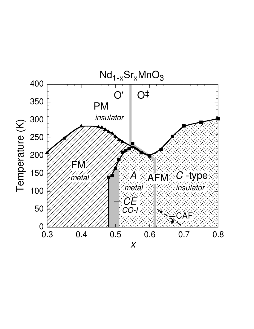
Figure 4: Magnetic phase diagram of Nd_1-xSr_xMnO₃ (from Ref. [32]). Different phases are denoted as follows: PM - paramagnetic, FM - ferromagnetic, and AFM - antiferromagnetic, consisting of the FM layers (A), simple chains (C), and zigzag chains (CE).

Typically, the CMR effect occurs at the boundary of either FM and PM, or FM and AFM phases. In this sense, the understanding of the magnetic phase diagram is directly related with the understanding of the CMR effect. There is a large number of modern review articles devoted to these compounds [26, 33, 34, 35], which covers a lot of experimental information as well as the theoretical views on the problem. In this section we would like to illustrate, as we believe, the main idea behind the magnetic phase diagram and the CMR effect itself from the viewpoint of electronic structure calculations and the general theory of interatomic magnetic interactions presented in Sec. 2. We will concentrate on the doping range $x$$\geq$$0.3$.

According to the formal valence arguments, the $3d$ states of Mn in $R_{1-x}D_{x}$MnO₃ are filled by the $(4$$-$$x)$ electrons, which are subjected to the strong Hund’s rule coupling. Therefore, the intra-atomic exchange splitting between the $\uparrow$- and $\downarrow$-spin $3d$ states can be regarded as the largest parameter in the problem. The $3d$ states are further split by the cubic crystal-field into the lower-lying $t_{2g}$ and higher-lying $e_{g}$ levels, yielding the formal electronic configuration $t_{2g\uparrow}^{3}e_{g\uparrow}^{1-x}t_{2g\downarrow}^{0}e_{g\downarrow}^{0}$. The band dispersion, caused by the interatomic hopping interactions involving $t_{2g}$ and $e_{g}$ orbitals is typically smaller than the intra-atomic exchange and crystal-field splittings. The hoppings are mediated by the oxygen $2p$ states, and in the undistorted cubic lattice are allowed only between orbitals of the same, either $t_{2g}$ or $e_{g}$, symmetry. The strengths of the Mn($e_{g}$)-O($2p$) and Mn($t_{2g}$)-O($2p$) interactions are controlled by the Slater-Koster parameters, correspondingly $pd\sigma$ and $pd\pi$. Since $|pd\sigma|$$>$$|pd\pi|$, the $t_{2g}$ band is typically narrower than the $e_{g}$ one [36].

Thus, the $t_{2g}$ states will be half-filled and according to Sec. 3.1 contribute only to the AFM SE interactions. The $e_{g}$ states are partially occupied and therefore will contribute to both FM DE and AFM SE interactions, whose ratio will depend on $x$.

What is the relevance of this picture to the magnetic phase diagram of perovskite manganites? In order to get a very rough idea about this problem, let us simply count the number of FM ($z_{\rm FM}$) and AFM ($z_{\rm AFM}$) bonds formed by the Mn sites in each of the magnetic phases shown in Fig. 4 (Table 2).

Table 2: Number of ferromagnetic ($z_{\rm FM}$) and antiferromagnetic ($z_{\rm AFM}$) bonds for the main magnetic phases observed in Nd_1-xSr_xMnO₃.

phase	$x$ in phase diagram	$z_{\rm FM}$	$z_{\rm AFM}$
FM	$0.3$$\leq$$x$$<$$0.5$	6	0
CE	$x$$\sim$$0.5$	2	4
A	$0.5$$\leq$$x$$\leq$$0.6$	4	2
C	$x$$>$$0.6$	2	4
G	$x$$\sim$$1$	0	6

The FM interactions prevail at smaller $x$. However, further increase of $x$ leads to the gradual change of the character of magnetic interactions towards the antiferromagnetism, which is reflected in the increase of the number of AFM bonds. Therefore, it seems reasonable to link this phase diagram with some kind of competition between FM and AFM interactions.

In order to further proceed with this picture, we need to address the following questions.

1. Which mechanism stabilizes the anisotropic AFM A and C structures in the metallic regime? Note, that according to the canonical DE model [7], the metallic antiferromagnetism is unstable with respect to a spin-canting.

2. What is so special about the CE phase? Why does it exist only in the narrow window of $x$ close to $x$$=$$0.5$ and perturbs the monotonous change of $z_{\rm FM}$ and $z_{\rm AFM}$ shown in Table 2? Why is it insulator?

3. Quantitative description of the doping-dependance of the magnetic phase diagram.

5.1.1 Basic Details of the Electronic Structure

The key factor factor, which allows to resolve the questions summarized in parts 1 and 2 is the strong dependance of the electronic structure of the $e_{g}$ states on the magnetic structure [37, 38, 39]. The effect can be estimated in the LSDA by considering the distribution of the $e_{g}$ states in the hypothetical virtual-crystal alloy La_1/2Ba_1/2MnO₃ (Fig. 5).

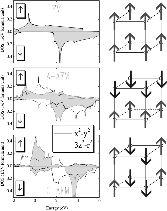
Figure 5: Distribution of the Mn($e_{g}$) states in the ferromagnetic, A-, and C-type antiferromagnetic phases of La_1/2Ba_1/2MnO₃ in LSDA. The Fermi level is at zero.

In this calculations, the crystal structure of La_1/2Ba_1/2MnO₃ was rigidly fixed to be the cubic one. Hence, Fig. 5 shows the pure response of the electronic structure of the $e_{g}$ states to the change of the magnetic structure. Even in LSDA, which typically underestimates the intra-atomic splitting between the $\uparrow$- and $\downarrow$-spin states [40], the effect is very strong and the electronic structure changes dramatically upon switching between FM, A-, and C-type AFM phases. Furthermore, the anisotropic AFM ordering has different effect on different $e_{g}$ orbitals. For example, in the A-type AFM structure, the main lobes of the $x^{2}$-$y^{2}$ and $3z^{2}$-$r^{2}$ orbitals are aligned correspondingly along FM and AFM bonds. Since the hopping interactions are penalized in the case of the AFM coupling, the A-type AFM arrangement will shrink mainly the $3z^{2}$-$r^{2}$ band. The effect is reversed in the C-type AFM state, which is associated with the narrowing of the $x^{2}$-$y^{2}$ band. Thus, the LSDA calculations clearly demonstrate how the anisotropy of the A- and C-type AFM structures interplays with the anisotropy of the spacial distribution of the $x^{2}$-$y^{2}$ and $3z^{2}$-$r^{2}$ orbitals.

The AFM CE phase presents the most striking example of such interplay between spin and orbital degrees of freedom: the zigzag AFM arrangement appears to be sufficient to explain the insulating behavior of this phase (even in LSDA). Therefore, the CE phase can be regarded as a band insulator, which is related with the very peculiar form of the AFM spin ordering (Fig. 6) [41].

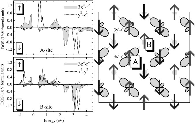
Figure 6: Right panel. Two-dimensional zigzag antiferromagnetic ordering realized in La_1/2Sr_3/2MnO₄, resulting in two different sublattices of the Mn sites (A and B, typically referred to the ”charge ordering”) and the orbital ordering (the alternation of partially populated $3x^{2}$-$r^{2}$ and $3y^{2}$-$r^{2}$ orbitals at the A sites). Left panel. Corresponding distribution of the Mn($e_{g}$) states at the sites A and B in LSDA. The Fermi level is at zero.

The magnetic-state dependence of the electronic structure of the $e_{g}$ states is the main microscopic mechanism, which stands behind the rich variety of the magnetic structures observed in perovskite manganites. In some sense, these systems show certain tendency to the self-organization, the main idea of which can be accumulated in the following formula: the anisotropic AFM ordering breaks the cubic symmetry of the crystal and leads to the strong anisotropy of the electronic structure. This anisotropy will be reflected in the anisotropy of interatomic magnetic interactions (8), which depend on the electronic structure through the matrix elements of the Green function. In many cases, the response of interatomic magnetic interactions to the change of the magnetic structure appears to be sufficient to explain the local stability of this magnetic state, and the total energy of such systems will have many local minima corresponding to different magnetic phases.

5.1.2 Minimal Model for CMR Manganites

The semi-quantitative model for CMR manganites can be constructed by using the following arguments.

• The model should be based on the realistic electronic structure for the $e_{g}$ states and take into account strong dependence of this electronic structure on the magnetic structure. The proper model for the electronic structure can be obtained by doing the tight-binding parametrization of LDA bands [36, 43]. However, for many applications one can use even cruder approximation and consider only the NN hoppings between Mn sites, parameterized according to Slater and Koster [44]:

  $$t_{\bm{\tau}\bm{\tau}+{\bf n}_{\alpha}}=\frac{t_{0}}{2}-\frac{t_{0}}{2}\left(\sin\frac{2\pi\alpha}{3}\sigma_{x}+\cos\frac{2\pi\alpha}{3}\sigma_{z}\right),$$

  where $t_{\bm{\tau}\bm{\tau}^{\prime}}$$\equiv$$\|t_{\bm{\tau}\bm{\tau}^{\prime}}^{LL^{\prime}}\|$ is the $2$$\times$$2$ matrix in the basis of two $e_{g}$ orbitals $x^{2}$-$y^{2}$ ($L$,$L^{\prime}$$=$$1$) and $3z^{2}$-$r^{2}$ ($L$,$L^{\prime}$$=$$2$), and ${\bf n}_{\alpha}$ is the primitive translation in the cubic lattice parallel to the $x$ ($\alpha$$=$$1$), $y$ ($\alpha$$=$$2$), or $z$ ($\alpha$$=$$3$) axis. The anisotropy of the $x^{2}$-$y^{2}$ and $3z^{2}$-$r^{2}$ orbitals is reflected in the anisotropy of transfer interactions. The parameter $t_{0}$$\propto$$(pd\sigma)^{2}$ is chosen to reproduce the $e_{g}$ bandwidth in LDA ($t_{0}$$\simeq$$0.7$ eV [26], and thereafter used as the energy unit).

  The effect of the magnetic structure on the electronic structure is typically included after transformation to the local coordinate frame, specified by the directions $\{{\bf e}_{\bm{\tau}}\}$ of the spin magnetic moments

  $${\bf e}_{\bm{\tau}}=\left(\cos\phi_{\bm{\tau}}\sin\theta_{\bm{\tau}},\sin\phi_{\bm{\tau}}\sin\theta_{\bm{\tau}},\cos\theta_{\bm{\tau}}\right),$$

  and taking the limit of infinite intra-atomic exchange splitting. This yields the well-known DE Hamiltonian [45]:

  $${\cal H}^{D}_{\bm{\tau}\bm{\tau}^{\prime}}=-\xi_{\bm{\tau}\bm{\tau}^{\prime}}t_{\bm{\tau}\bm{\tau}^{\prime}},$$ (12)

  where

  $$\xi_{\bm{\tau}\bm{\tau}^{\prime}}=\cos\frac{\theta_{\bm{\tau}}}{2}\cos\frac{\theta_{\bm{\tau}^{\prime}}}{2}+\sin\frac{\theta_{\bm{\tau}}}{2}\sin\frac{\theta_{\bm{\tau}^{\prime}}}{2}e^{-i(\phi_{\bm{\tau}}-\phi_{\bm{\tau}^{\prime}})}$$

  describes modulations of transfer interactions caused by deviations from the FM spin alignment.

• ${\cal H}^{D}_{\bm{\tau}\bm{\tau}^{\prime}}$ is proportional to $t_{0}$, and similar to the DE term considered in Sec. 3.1, describes the FM interactions in the systems, which are now generalized to the case of arbitrary spin arrangement. This term is combined with the energy of phenomenological AFM SE interactions:

  $${\cal H}^{S}_{\bm{\tau}\bm{\tau}^{\prime}}=-\frac{1}{2}J^{S}{\bf e}_{\bm{\tau}}\cdot{\bf e}_{\bm{\tau}^{\prime}},$$

  where $J^{S}$$<$$0$ is restricted by the nearest neighbors and contains contributions of both $t_{2g}$ and $e_{g}$ states. Using an analogy with the SE model considered in Sec. 3.2, it is assumed that the exchange constant $J^{S}$ does not depend on the magnetic state, and all such dependencies come exclusively from the DE term.

The combination of ${\cal H}^{D}_{\bm{\tau}\bm{\tau}^{\prime}}$ and ${\cal H}^{S}_{\bm{\tau}\bm{\tau}^{\prime}}$ constitutes the minimal model, which explains the origin of the main magnetic structures observed in doped manganites. An example of theoretical phase diagram is shown in Fig. 7 [37, 38, 50].

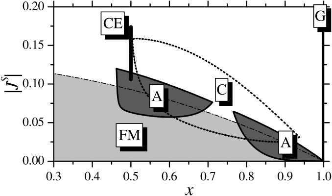
Figure 7: The areas of local stability of the main collinear phases with respect to the spin canting in the degenerate double exchange model (from Ref. [38]).

The position and the order of the main magnetic phases with respect to the hole-doping has clear similarity with the experimental phase diagram (Fig. 4).

The origin of the CE-type AFM phase requires special comment, because canonically it was attributed to the charge ordering of the Mn³⁺ and Mn⁴⁺ ions [1], and this point of view was dominating for many years. The modern view on the problem is that CE is the regular magnetic phase, whose properties can be understood in the degenerate DE model similar to other magnetic states [26, 35, 39]. The insulating behavior of this phase is related with the topology of one-dimensional zigzag FM chains. This also explains why the CE phase exists in the very narrow region close to $x$$=$$0.5$, i.e. when the Fermi energy falls into the band gap. More generally, any periodic one-dimensional zigzag object composed of the $e_{g}$ orbitals will behave as a band insulator at certain commensurate values of the electron density [26, 51].

5.1.3 Implication to the CMR Effect

The magnetic origin of the CE phase has many implications to the CMR effect and readily explains why the insulating state of some manganites can be easily destroyed by the external magnetic field. However, it would not be right to say that CMR is exclusively related with the existence of the CE phase. It is a more general phenomenon inherent to the DE physics. Below we will consider two such possibility.

1. According to the form of the DE Hamiltonian (12), the transfer interactions are forbidden between antiferromagnetically coupled sites. Therefore, from the viewpoint of transport properties, the A-type AFM phase behaves as an insulator in the $z$-directions and as a metal in the $xy$-plane. The A state can be continuously transformed to the spin-canted state [38] by applying the external magnetic field. The spin-canting unblocks the hopping interactions and gradually decreases the resistivity along $z$. This is the basic idea of the so-called ”spin-valve” effect, observed in the A-type AFM Nd_0.45Sr_0.55MnO₃ [52].

The unique aspect of the CE phase is that it has a band gap, and therefore is insulating in all the directions, including the direction of propagation of the FM zigzag chains. This predetermines rather distinguished behavior of the CE phase in the magnetic field. As it was pointed out before, the stability of the CE phase is directly related with the existence of the band gap. Similar to the A-type AFM phase, the external magnetic field leads to the canting of spins also in the CE phase. The basic difference is that starting with certain angle such canting will close the band gap. Then, the CE phase will become unstable and the system will abruptly transform to the metallic FM phase, which is favored by the magnetic field. The phenomenon is well know as the ”melting of the charge-ordered state”, which accompanied by the abrupt drop of the resistivity [34].

2. Typical theories of the second type are based on the following observations [53]:

• The total energy of the DE model may have several local minima corresponding to different FM and AFM phases, which may exist in the same range of the hole-doping. This also implies the first-order character of the phase boundaries [50]. The concrete example is the region close to $x$$=$$0.5$ shown in Fig. 7.

• Some of these phases are insulating due to the special (zigzag) geometry of the AFM pattern.

The situation is schematically illustrated in Fig. 8.

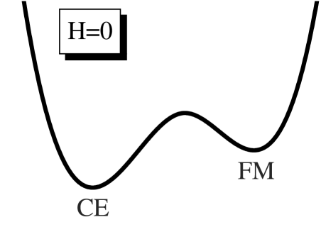
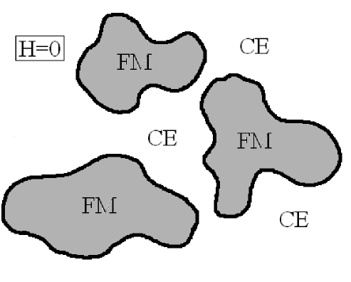
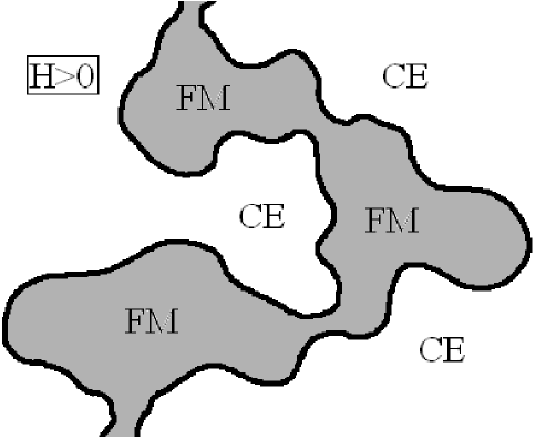
Figure 8: Schematic view on the percolative scenario of the CMR effect. Top: Local minima of the double exchange energy corresponding to the insulating CE and metallic FM phases. The relative position of these minima is controlled by the magnetic field $H$. Bottom: mixed-phase state realized at the finite temperature. The magnetic field increases the amount of the FM phase, and above the percolation threshold forms the conducting FM path.

At $T$$=$$0$ and without field, the system is trapped in the insulating CE-type AFM ground state. The next minimum, corresponding to the FM metallic state should be located within the energy range accessible by the external magnetic field. At the finite temperature and neglecting interactions between different phases, the system will be represented by the mixture of these two states, due to the configuration mixture entropy. The relative amount of these states will depend on the temperature $T$ and the magnetic field $H$. The latter controls the relative position of the CE and FM minima. Without field, the CE phase will dominate, while the FM phase will form metallic islands in the insulating sea. The application of the magnetic field will increase the amount of the of the FM phase. At some point, which is called the percolation threshold, the FM islands become connected by forming the conducting FM paths throughout the spacemen. This will correspond to the sharp drop of the resistivity.

Since many interesting (and, presumably, the most practical) phenomena of perovskite manganites are related with the existence of zigzag AFM structures, it is very important to understand the behavior of these structures, and especially the way how they will evolve with the temperature, in the magnetic field, or upon the change of the crystal structure. We would like to close this section by listing some interesting and not completely resolved problems in this direction.

• The existence of two transition temperatures, $T_{\rm N}$ and $T_{\rm CO}$, which are typically attributed to the onset of Néel AFM and charge ordering, respectively. In reality, both transitions are probably magnetic and $T_{\rm N}$ corresponds to the order-disorder transition which takes place only between FM zigzag chains and largely preserves the coherent motion of spins within the chains, while $T_{\rm CO}$ corresponds to the transition to the totally disordered PM state [55].

• Appearance of incommensurate charge and orbital superstructures just below $T_{\rm CO}$ [56].

• Effects of cation disorder and appearance of new zigzag superlattices upon artificial ordering of $R$ and $D$ elements in some three-dimensional manganites [57].

5.1.4 Role of Rare-earth, Alkaline-earth, and Oxygen and States

In this section we will briefly discuss the influence of the $R$, $D$, and oxygen states on the interatomic magnetic interactions in $R_{1-x}D_{x}$MnO₃ in the context of revisions in the form of these interactions, which were recently considered by Bruno [20]. We will concentrate on the behavior of the cubic FM phase of the virtual-crystal alloy La_0.7Ba_0.3MnO₃, and treat the problem of interatomic magnetic interactions using the frozen spin wave approximation supplemented with the LSDA. In the FM phase, the magnetic Mn sites polarize neighboring La/Ba and oxygen sites. The typical distribution of the magnetic moments amongst different sites is $\mu_{\rm Mn}$$=$$3.48$, $\mu_{\rm La/Ba}$$=$$0.08$, and $\mu_{\rm O}$$=$$0.05$ $\mu_{B}$. Our main concern will be the role played by $\mu_{\rm La/Ba}$ and $\mu_{\rm O}$ in the spin dynamics of La_1-xBa_xMnO₃.

We assume that the cone-angle of the spin wave does not depend on the atomic site: $\theta_{\bm{\tau}}$$\equiv$$\theta$. The phase of the spin wave is modulated as ${\bf q}\cdot\bm{\tau}$ with $\bm{\tau}$ running over all Mn, O, and La/Ba sites. Then, for each ${\bf q}$ we calculate the second derivative of the total energy with respect to $\theta$ using the magnetic force theorem. The derivative can be also used to estimate the magnon spectrum in the FM state:

$$\omega_{\bf q}=\frac{2}{\mu}\left.\frac{d^{2}E({\bf q},\theta)}{d\theta^{2}}\right|_{\theta=0}$$

($\mu$ being the FM moment). We consider two possibility:

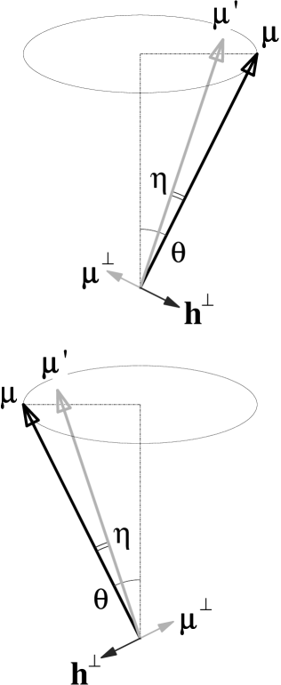
Figure 9: Typical situation realized in frozen spin wave calculations for ${\bf q}$$=$$(0,0,\pi)$. $\{\bm{\mu}\}$ is the constrained distribution of the magnetic moments. $\{\bm{\mu}^{\prime}\}$ is the distribution of magnetic moments obtained after solution of Kohn-Sham equations with the rotated effective fields. Generally, the spins $\{\bm{\mu}^{\prime}\}$ are canted towards the ground state configuration by the angle $\eta$, and have the components $\{\bm{\mu}^{\perp}\}$, which are perpendicular to $\{\bm{\mu}\}$. The constraining fields $\{{\bf h}^{\perp}\}$ are included in order to compensate $\{\bm{\mu}^{\perp}\}$.

• Rigid constraint, obtained by rotating the KS effective field and enforcing the directions of the spin magnetic moments at each site to follow exactly the form of the spin wave. The latter is achieved by applying the perpendicular constraining fields $\{{\bf h}^{\perp}_{\bm{\tau}}\}$ (Fig. 9), which can be estimated using the response-type arguments [20]. The fields $\{{\bf h}^{\perp}_{\bm{\tau}}\}$ affect the KS orbitals $\{\psi_{i}\}$, and through the change of these orbitals, correct the form of the spin-magnetization density (2). However, they do not contribute explicitly to the total energy change (5).

• Relaxed constraint, obtained after rotation of the KS effective fields.

Results of these calculations are shown in Fig. 10.

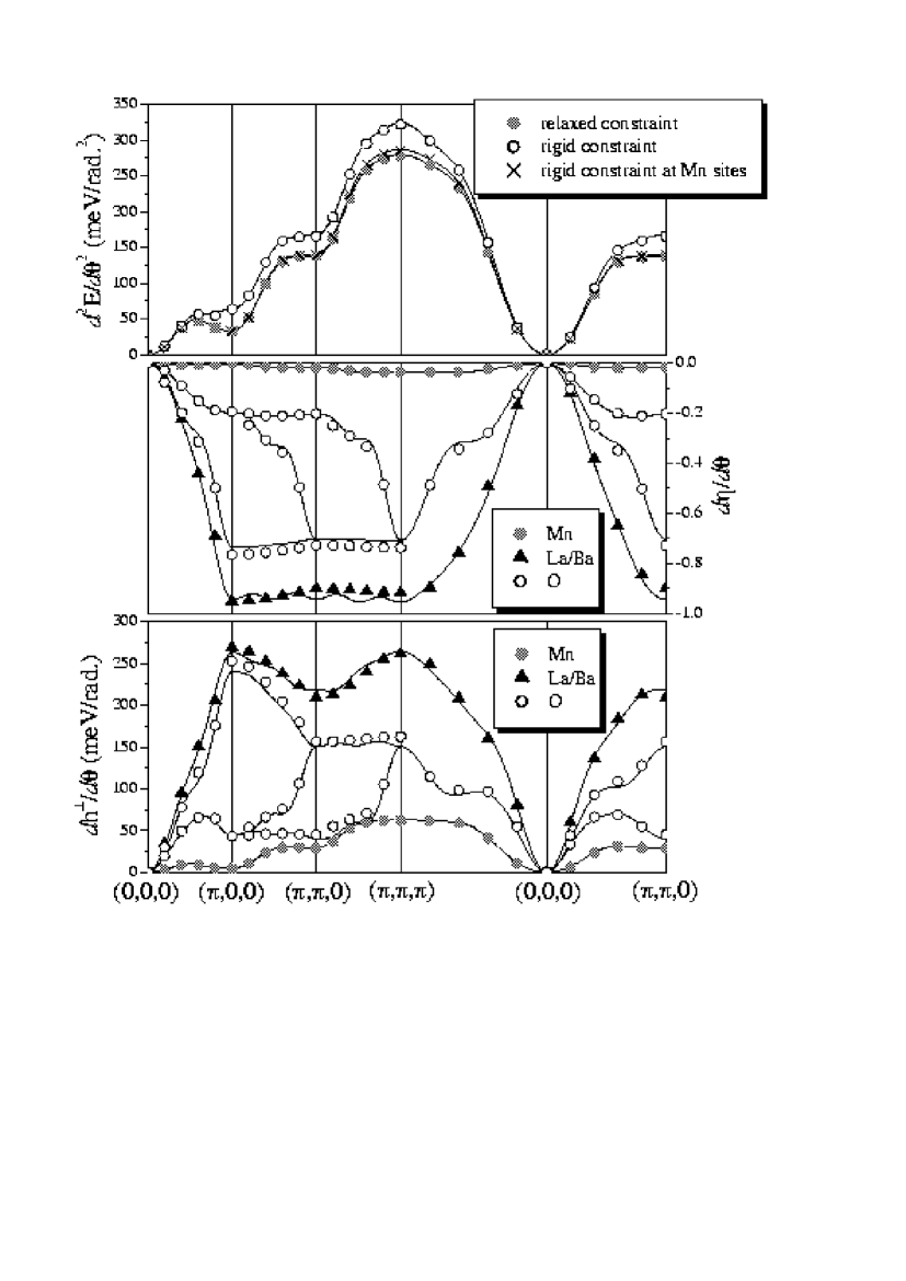
Figure 10: Results of frozen spin wave calculations for La_0.7Ba_0.3MnO₃: second derivatives of the total energy (which specify the form of the magnon dispersion) obtained by rotating the Kohn-Sham effective fields (relaxed constraint) and by applying additional perpendicular constraining fields $\{{\bf h}^{\perp}_{\bm{\tau}}\}$ (rigid constraint) at all sites and the Mn sites only; the parasitic canting of the magnetic moments in the relaxed constraint calculations; and the perpendicular magnetic field applied in order to compensate this canting. Symbols show the calculated points, and the solid lines are results of an interpolation.

The magnon dispersion has a characteristic form, which is manifested in the pronounced softening at the Brillouin zone boundaries [58]. The origin of this softening is related with the behavior of interatomic magnetic interactions, and can be understood on the basis of realistic electronic structure calculations [25]. It has a direct implication to the stability of the FM state and the form of the magnetic phase diagram versus the hole-doping [26].

In this section, our main concern will be a little bit different. As it is seen in Fig. 10, the application of the constraining fields $\{{\bf h}^{\perp}_{\bm{\tau}}\}$ can significantly affect the magnon dispersion. For example, around $(\pi,0,0)$, $\omega_{\bf q}$’s calculated using two different schemes can differ by factor two. The most interesting question is where this difference comes from. The simple rotation of the KS effective fields by the angle $\theta$ causes the parasitic canting of spins off the constrained directions by the angles $\{\eta_{\bm{\tau}}\}$, which are proportional to $\theta$ if the latter is small (see Fig. 9). However, this canting can be very different at different magnetic sites. Indeed, $\eta_{\bm{\tau}}$ is of the order of $\theta$ at the La/Ba and oxygen sites, and almost negligible at the Mn sites. Therefore, the fields $\{{\bf h}^{\perp}_{\bm{\tau}}\}$, which are introduced in order to correct this canting will be the largest at the La/Ba and oxygen sites, and the smallest at the Mn sites. An attempt to apply ${\bf h}^{\perp}_{\bm{\tau}}$ only at the Mn sites has a negligible effect on the magnon dispersion. These results rise several important questions, which still need to be understood.

$\bullet$ There is a large intrinsic uncertainty in the behavior of spin magnetization at the La/Ba and oxygen sites, and especially in the form, in which these sites contribute to the spin dynamics of La_1-xBa_xMnO₃ and similar compounds. The problem may be directly related with the definition of the adiabaticity concept, underlying the frozen spin wave approach. According to this concept, the magnetic systems have two characteristic time scales. The spin directions are typically regarded as the slow variables, while the internal electronic degrees of freedom are the fast ones, which self-consistently follow the instantaneous orientational distribution of the spin-magnetization density. From this point of view, the La/Ba and oxygen sites have clearly a dual character. On the one hand, neither of them can be regarded as the source of magnetism in these systems. On the other hand, both of them carry a significant weight of the spin-magnetization density, mainly due to the hybridization with the magnetic Mn sites. Then, how the La/Ba and oxygen states shall be treated? In principle, one may have several possibilities.

1. The La/Ba and oxygen sites are magnetic and shell be treated on the same level as the Mn sites, by applying independent constraint conditions for the slow-varying directions of the La/Ba and oxygen spins. This would correspond to the appearance of additional magnon branches in the frozen spin wave calculations. Clearly, this scenario can be sorted out from the beginning, because both La/Ba and oxygen moments are induced by the hybridization with the Mn sites and cannot be totally independent from the latter.

2. The contribution of La/Ba and oxygen states is purely electronic, which implies that these degrees of freedom are ”fast” and self-consistently follow the distribution of the spin magnetic moments at the Mn sites. This would roughly correspond to the relaxed constraint conditions in the spin-wave calculations shown in Fig. 10.

3. An intermediate situation when the electronic degrees of freedom at the La/Ba and oxygen sites are not ”sufficiently fast” so that the magnon dispersion shall be averaged over several intermediate configurations of the La/Ba and oxygen spins. This is the most interesting scenario, which is however only a speculation. If true, the magnon dispersion in FM manganites should have an intrinsic bandwidth, which should be of the same order of magnitude as the difference between ”rigid” and ”relaxed” calculations shown in Fig. 10. In fact, the strong magnon broadening has been observed experimentally in several FM manganites [58], though it is of course premature to make a direct connection between this broadening and the behavior of La/Ba and oxygen states considered in this section.

$\bullet$ The non-collinear distribution of magnetic moments at the La/Ba and oxygen sites can interfere with other (extrinsic) factors, such as randomness effects caused by the cation disorder. Then, the chemical disorder may lead to the orientational spin disorder at the La/Ba and oxygen sites, which may also contribute to the magnon broadening associated with the randomness [59].

5.2 Double Perovskites

Ordered double perovskites, like Sr₂FeMoO₆ and Sr₂FeReO₆, is another interesting class of compounds [60]. They exhibit fairly large magneto-resistance effect, which coexists with relatively high magnetic transition temperature (415 and 401 K for Sr₂FeMoO₆ and Sr₂FeReO₆, respectively). The latter factor presents a great advantage over CMR manganites, and opens a way to technological applications of these compounds in devices operating at the room temperature.

At the first sight, the double perovskites crystallize in a simple crystal structure. It can be regarded as the cubic SrFeO₃, in which every second Fe is replaced by Mo or Re (Fig. 11).

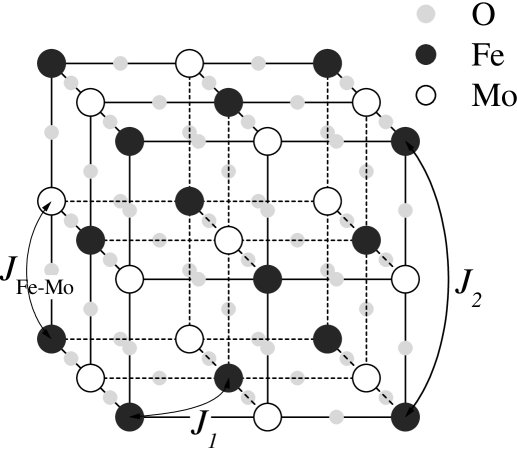
Figure 11: Positions of Fe, Mo, and oxygen sites in ordered double perovskite Sr₂FeMoO₆. Arrows show the main magnetic interactions responsible for properties of this compound.

However, there are two fundamental problems:

1. Anti-site defects. Typically, certain percent of atoms from the nominally Fe sublattice interchanges with the same amount of atoms from the Mo sublattice. The number of such defects in the best available single-crystalline samples of Sr₂FeMoO₆ is about 8% [61].

2. Fine details of the crystal structure. Typically, the information about directions and magnitudes of the oxygen displacement is either unknown or rather controversial.

The extraordinary properties of Sr₂FeMoO₆ and Sr₂FeReO₆ are usually attributed to the half-metallic electronic structure expected in the FM state. In this sense, the double perovskites are typically considered as an example of relatively simple and well established physics.

In this section, we will discuss the behavior of interatomic magnetic interactions in Sr₂FeMoO₆ and argue that this point of view must be largely revised. Particularly, we will show that the half-metallic electronic structure is incompatible with stability of the FM ground state. Therefore, there should be some additional mechanism which stabilizes the FM state and presumably destroys the half-metallic character of the electronic structure. We propose that the unique properties of the double perovskites are directly related with the above-mentioned defects and uncertainties of the crystal structure [62].

A rough idea about the problem can be obtained from rather simple considerations of the electronic structure of Sr₂FeMoO₆ (Fig. 12), which suggests that similar to the CMR manganites there are two competing interactions which define the form of the magnetic ground state in this compound.

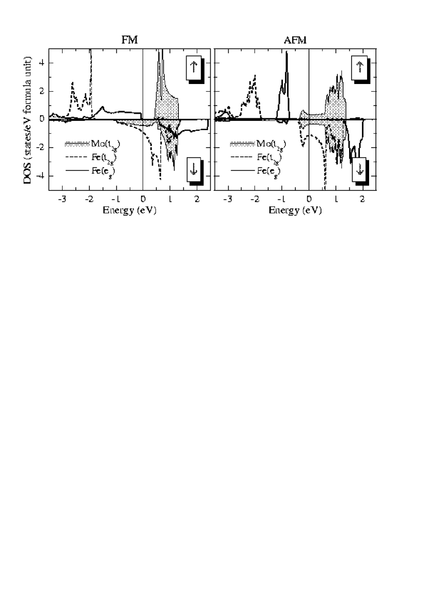
Figure 12: Local densities of states corresponding to the ferromagnetic (left) antiferromagnetic (right) alignment of Fe spins in ordered Sr₂FeMoO₆, in LSDA. The Fermi level is at zero.

1. It is true that the electronic structure of the hypothetical FM phase of Sr₂FeMoO₆ is half-metallic: the Fermi level crosses the hybrid $t_{2g}$ band in the $\downarrow$-spin channel and falls in the gap between Fe($e_{g}$) and Mo($t_{2g}$) bands in the $\uparrow$-spin channel. The partly-filled $\downarrow$-spin $t_{2g}$ band will generally be the source of FM interactions, due to the double exchange mechanism considered in Sec. 3.1, which will be somewhat modified by the fact that the transfer interactions between spin-polarized Fe($t_{2g}$) orbitals are indirect and operate via nonmagnetic Mo($t_{2g}$) states [63]. This interaction will also polarizes the Mo($t_{2g}$) states antiferromagnetically with respect to the Fe sublattice.

2. The half-filled Fe($e_{g}$) states should generally contribute to AFM interactions. Typically, this contribution is expected to be small, because in the double-perovskite structure, the neighboring Fe sites are separated by the long O-Mo-O paths. A very rough idea about the strength of these interactions can be obtained from the comparison of densities of the Fe($e_{g}$) states in the FM and (type-II [6]) AFM phases: if these interaction were weak, the bandwidth would not depend on the magnetic state. However, the direct calculations show the opposite trend and the Fe($e_{g}$) band considerably shrinks in the case of the AFM alignment.

A simple estimate of the relative strength of the FM and AFM contributions, irrespective on their decomposition onto the interatomic magnetic interactions, can be obtained from the one-electron (band) energies

$$E_{b}=\int\varepsilon{\cal N}(\varepsilon)d\varepsilon$$

(${\cal N}$ being the total density of states) calculated separately for the $e_{g}$ and $t_{2g}$ bands in the FM and AFM phases. These energies are listed in Table 3.

Table 3: One-electron energies associated with the hybrid $t_{2g}$ band located near the Fermi level and the occupied Fe($e_{g}$) band in the FM and AFM states of Sr₂FeMoO₆.

band	FM	AFM
$t_{2g}$	-1.8	-1.7
$e_{g}$	-4.6	-4.7

One can clearly see that in the AFM state, the energy loss associated with the hybrid $t_{2g}$ band is totally compensated by the energy gain associated with the Fe($e_{g}$) band. This example shows that the problem is indeed very subtle and the half-metallic electronic structure obtained in the FM state does not necessary guarantee that this state will be locally stable and realized as the ground state. It does not explain the high value of the magnetic transition temperature either.

The conclusion is supported by direct calculations of interatomic magnetic interactions using both frozen spin wave and Green’s function methods.

1. The FM state appears to be unstable with respect to the non-collinear spin-spiral alignment realized at certain ${\bf q}$’s, for which $\frac{d^{2}}{d\theta^{2}}\left.E({\bf q},\theta)\right|_{\theta=0}$$<$$0$ (Fig. 13).

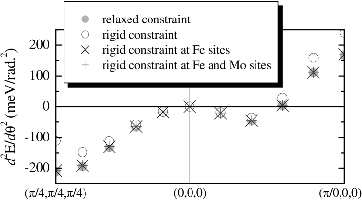
Figure 13: Results of frozen spin wave calculations for ordered Sr₂FeMoO₆ (see Fig. 10 for details).

The second derivative of the total energy was calculated using several different approximations, similar to the analysis of the spin-wave dispersion of La_0.7Sr_0.3MnO₃ undertaken in Sec. 5.1.4: by imposing the rigid constraint on the directions of spin magnetic moments at all sites of Sr₂FeMoO₆, and only at the Fe and Mo ones. Similar to the La_0.7Sr_0.3MnO₃ case, the main effect of the constraining fields $\{{\bf h}^{\perp}_{\bm{\tau}}\}$ is associated with the Sr and oxygen sites, whereas the contributions of the Fe and Mo sites are negligible. The ”rigid constraint” can be regarded as the most consistent check for the local stability of the FM state, when the application of the magnetic force theorem is strictly justified and the second derivative of the total energy can be rigorously expressed through the change of the KS single-particle energies. Fig. 13 shows that it may correct to a certain extent the values of the second derivatives at the Brillouin zone boundary. However, it does not change the principal conclusion and the FM state remains unstable in the large portion of the Brillouin zone [62].

2. The second derivatives of the total energy can be mapped onto the Heisenberg model $\frac{d^{2}}{d\theta^{2}}\left.E({\bf q},\theta)\right|_{\theta=0}$$=$$J_{0}$$-$$J_{\bf q}$. The mapping gives us parameters of magnetic interactions in the reciprocal space $\{J_{\bf q}\}$, which can be further transformed to the real space. The real-space parameters, listed in Table 4, provide a complementary piece of information which allows to rationalize results of frozen spin wave calculations and present them in terms of competition between FM NN and AFM next-NN interactions in the Fe sublattice (correspondingly $J_{1}$ and $J_{2}$ in Table 4).

Table 4: Parameters of magnetic interactions in the real space obtained in the (relaxed) frozen spin wave (SW) and Green’s function (GF) calculations near the FM and AFM states of Sr₂FeMoO₆ (in meV). Two values of $J_{1}$ in the case of the AFM alignment correspond to nearest-neighbor interactions between Fe sites having the same (the first number) and opposite (the second number) spins in the type-II antiferromagnetic structure.

method	$J_{1}$	$J_{2}$	$J_{\rm Fe-Mo}$
SW (FM)	9.3	-26.9	$-$
GF (FM)	6.2	-21.5	-1.2
SW (AFM)	16.4, 18.6	-15.2	0

The AFM interaction $J_{2}$ clearly dominates and readily explains why the FM state becomes unstable. An additional piece of information can be obtained from Green’s function calculations, which allow to estimate the direct Fe-Mo interaction $J_{\rm Fe-Mo}$. However, this interaction is not particularly strong and does not alter the main conclusion about stability of the FM state.

3. If the FM state is unstable, what is the true magnetic ground state of the ordered Sr₂FeMoO₆? The question is not simple, because the AFM phase appears to be also unstable, as it is expected for small concentrations of ($t_{2g}$) carriers moving in the AFM background of localized ($e_{g}$) spins and interacting with the latter via the strong intra-atomic Hund’s coupling [7]. This fact is also related with the magnetic-state dependence of interatomic magnetic interactions, which leads to the reversed inequality $J_{1}$$>$$|J_{2}|$ for parameters calculated in the AFM state (Table 4). Therefore, the true ground state of the chemically ordered Sr₂FeMoO₆ should lie in-between the FM and AFM states. The character of interatomic magnetic interactions suggests that probably it is a spin-spiral with ${\bf q}$$||$$[111]$.

The FM ordering can be stabilized by the anti-site defects or the local lattice distortions [62]. However, both mechanisms will destroy the half-metallic character of the electronic structure of Sr₂FeMoO₆. This is an irony of the situation. From the electronic structure point of view, the most efficient way to stabilize the ferromagnetism is to create holes in the $\uparrow$-spin Fe($e_{g}$) band, by shifting the Fermi level to the lower energy part of the spectrum, and thereby activate a very effective channel for the FM DE interactions associated with the $e_{g}$ states, similar to the CMR manganites.

Let us give a rough estimate for this effect. The width of the Fe($e_{g}$) band ($W$) in Sr₂FeMoO₆ is about 2 eV (Fig. 12), which is approximately two times smaller than the typical $e_{g}$ bandwidth in FM manganites. Therefore, the DE and SE interactions in Sr₂FeMoO₆, being proportional to $W$ and $W^{2}$, will be correspondingly two and four times smaller in comparison with the same interactions in manganites. The latter can be estimated as $J^{D}\simeq 80$ and $J^{S}\simeq-70$ meV, respectively [26]. Therefore, the partial depopulation of the $\uparrow$-spin Fe($e_{g}$) band in Sr₂FeMoO₆ leads the following estimate for next-nearest-neighbor coupling: $J_{2}\simeq\frac{1}{2}J^{D}+\frac{1}{4}J^{S}\simeq 20$ meV, which easily explains the appearance of ferromagnetism in this compound.

Thus, the half-metallic electronic structure realized in the FM state of the ordered double perovskites is a spurious effect since it is largely incompatible with stability of this FM state. It also implies that the 100% ordered double perovskites cannot be ferromagnetic. The latter observation is qualitatively consistent with the behavior of Sr₂FeWO₆, where almost perfect ordering of Fe and W coexists with an AFM ground state [64].

The quantitative theory of ferromagnetism in Sr₂FeMoO₆ and Sr₂FeReO₆ is still missing. The exceptionally high value of the Curie temperature is one of the main puzzles, which is probably related with the extrinsic inhomogeneities (anti-site defects, local lattice distortions, grain boundaries) existing in the samples. The magneto-resistive behavior is based on the percolative scenario, and is not necessary related with the half-metallic character of the electronic structure. The main difference from CMR manganites is that neither FM nor AFM states are locally stable and cannot be the total energy minima in the case of double perovskites. Therefore, the extrinsic inhomogeneity seems to be indispensable in order to stabilize the FM islands and form the two-pase state similar to the one depicted in Fig. 8. Then, the negative magneto-resistance may occur if the size of these islands can be easily controlled by the external magnetic field.

Finally, our analysis was based on the electronic structure obtained in LSDA, which may be imperfect. The role of Coulomb correlations on the top of LSDA is rather unclear. It is also unclear whether the Coulomb correlations alone can stabilize the FM state. On the one hand, the on-site $U$ enters the denominator for the SE interactions and therefore suppress the AFM contribution associated with the Fe($e_{g}$) states. On the other hand, it may change the relative position of the Fe and Mo states and thereby suppress the FM DE interactions associated with the hybrid $t_{2g}$ band [62]. We expect that the LSDA band structure depicts the main problems of the double perovskites, though the concrete details may depend on the Coulomb correlations on the top of this picture.

5.3 $A_{2}$Mo₂O₇ ($A$$=$ Y, Gd, and Nd) Pyrochlores

Pyrochlores with the chemical formula $A_{2}$Mo₂O₇ ($A$ being the divalent element) is one of the rare examples of magnetic oxides on the basis of $4d$ elements. The magnetic phase diagram of $A_{2}$Mo₂O₇ is controlled by the averaged ionic radius $\langle r_{A}\rangle$ of the $A$-sites. This dependence is very puzzling (Fig. 14) [66, 67, 68, 69].

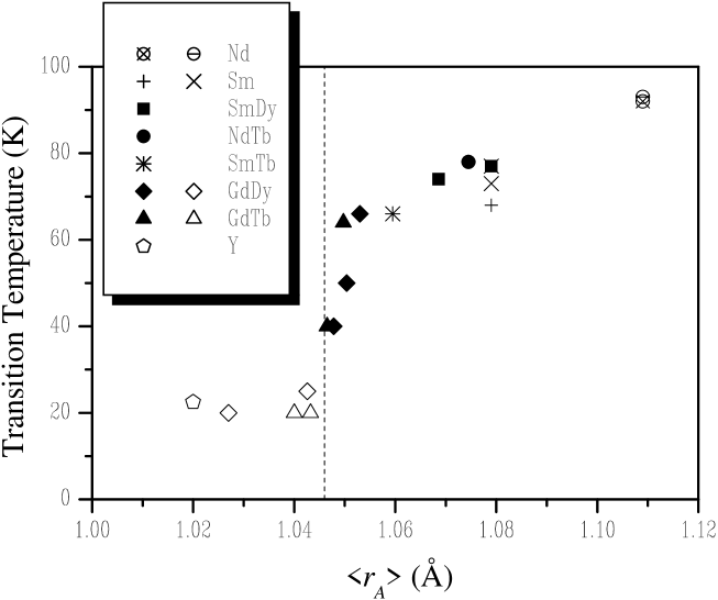
Figure 14: Experimental phase diagram of $A_{2}$Mo₂O₇: transition temperature against the averaged ionic radius. The dotted line shows the boundary between normal ferromagnetic (right) and spin-glass (left) behavior.

Large $\langle r_{A}\rangle$ ($>$$R_{c}$$\sim$$1.047$) stabilizes the ferromagnetic (FM) ground state. Typical examples of the FM pyrochlores are Nd₂Mo₂O₇ and Gd₂Mo₂O₇. The Curie temperature ($T_{C}$) is of the order of 80 K and slowly increases with $\langle r_{A}\rangle$. Smaller $\langle r_{A}\rangle$ ($<$$R_{c}$) give rise to the spin-glass (SG) behavior. The characteristic transition temperature to the SG state is of the order of 20 K. The canonical example of the SG compounds is Y₂Mo₂O₇ [70]. Intuitively, it is clear that such a behavior should be related with the change of the NN exchange coupling, which becomes antiferromagnetic in the SG region. The pyrochlore lattice supplemented with the AFM exchange interactions presents a typical example of geometrically frustrated systems with an infinitely degenerate magnetic ground state [71], which probably predetermines the SG behavior. The FM-SG transition in Mo pyrochlores is closely related with the metal-insulator transition. All compounds which reveal the SG behavior are small-gap insulators. However, the opposite statement is generally incorrect and in different compounds the ferromagnetism is known to coexist with the metallic as well as the insulating behavior [69]. In this section we will try to understand which parameter of the crystal structure controls the sign of the NN magnetic interactions, and which part of the electronic structure is responsible for the FM and AFM interactions in these compounds.

5.3.1 Main Details of Crystal and Electronic Structure

The pyrochlores $A_{2}$Mo₂O₇ crystallize in a face-centered cubic structure with the space group $Fm\overline{3}d$, in which $A$ and Mo occupy correspondingly $16d$ and $16c$ positions, and form interpenetrating sublattices of corner-sharing tetrahedra. There is only one internal parameter which may control the properties of $A_{2}$Mo₂O₇. That is the coordinate $u$ of the O $48f$ sites.

The single Mo tetrahedron is shown in Fig. 15.

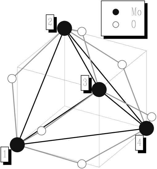
Figure 15: Positions of the Mo and O $48f$ sites in the pyrochlore lattice.

Four Mo sites are located at $\bm{\tau}_{1}$$=$$(0,0,0)$, $\bm{\tau}_{2}$$=$$(0,\frac{1}{4},\frac{1}{4})$, $\bm{\tau}_{3}$$=$$(\frac{1}{4},0,\frac{1}{4})$, and $\bm{\tau}_{4}$$=$$(\frac{1}{4},\frac{1}{4},0)$, in units of cubic lattice parameter $a$. Each Mo site has sixfold O $48f$ coordination. The oxygen atoms specify the local coordinate frame around each Mo site. Around 1, it is given by

$${\cal R}_{1}^{\alpha\beta}=\frac{1+(1-8u)\delta_{\alpha\beta}}{\sqrt{64u^{2}-32u+6}},$$ (13)

where $\alpha,\beta$$=$ $x$, $y$, or $z$. $u$$=$$\frac{5}{16}$ corresponds to the perfect octahedral environment, while $u$$>$$\frac{5}{16}$ gives rise to an additional trigonal contraction of the local coordinate frame. Similar matrices associated with the sites 2, 3, and 4 can be obtained by the $180^{\circ}$ rotations of $\widehat{\cal R}_{1}$ around $x$, $y$, and $z$, respectively.

Structural parameters of $A_{2}$Mo₂O₇ (taken from Refs. [66, 67, 68, 69, 70]) are listed in Table 5.

Table 5: Structural parameters of $A_{2}$Mo₂O₇ ($A$$=$ Y, Nd, and Gd): the cubic lattice parameter $a$ (in Å), positions of O $48f$ sites $[u,\frac{1}{8},\frac{1}{8}]$ (units of $a$), the distances Mo-Mo (in Å), and the angles Mo-O-Mo (in degrees).

compound	$a$	$u$	$d_{\rm Mo-Mo}$	$\angle$Mo-O-Mo
Y2Mo2O7	10.21	0.33821	3.6098	127.0
Gd2Mo2O7	10.3356	0.33158	3.6542	130.4
Nd2Mo2O7	10.4836	0.32977	3.7065	131.4

Corresponding densities of states, obtained in LSDA are shown in Figs. 16 and 17.

Figure 16: Total and partial densities of states of Nd₂Mo₂O₇ in the local-spin-density approximation. The Mo($t_{2g}$) states are located near the Fermi level (chosen as zero of energy). The Mo($e_{g}$) states emerge around 4 eV.

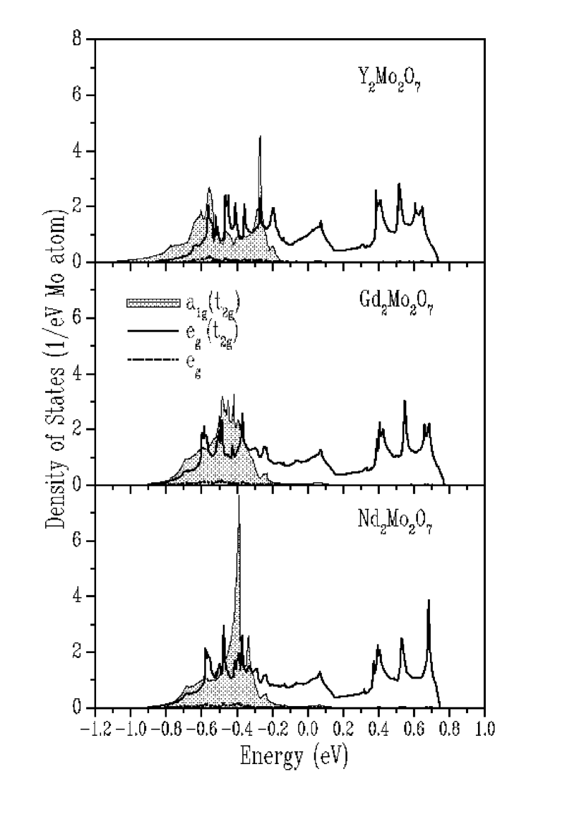
Figure 17: Mo($t_{2g}$) states in the local coordinate frame, split into the one-dimensional $a_{1g}$ and two-dimensional $e_{g}^{\prime}$$=$$e_{g}$($t_{2g}$) representations by the local trigonal distortion.

In the local coordinate frame, the Mo($4d$) orbitals are split into the triply-degenerate $t_{2g}$ and doubly-degenerate $e_{g}$ states. Twelve $t_{2g}$ bands are located near the Fermi level and well separated from the rest of the spectrum. Interestingly enough that all three compounds $A_{2}$Mo₂O₇ ($A$$=$ Y, Gd, and Nd) are ferromagnetic, even in LSDA, that is rather unusual for the $4d$ oxides, perhaps except the well know example of SrRuO₃ [73]. The trigonal distortion and the different hybridization with the O($2p$) states will further split the Mo($t_{2g}$) states into the one-dimensional $a_{1g}$ and two-dimensional $e_{g}^{\prime}$ representations. The crystal structure affects the Mo($t_{2g}$) bandwidth via two mechanisms (see Table 5).

1. The Mo-O-Mo angle, which decreases in the direction Nd$\rightarrow$Gd$\rightarrow$Y. Therefore, the interactions between Mo($t_{2g}$) orbitals which are mediated by the O($2p$) states will also decrease.

2. The lattice parameter $a$ and the Mo-Mo distance, which decrease in the direction Nd$\rightarrow$Gd$\rightarrow$Y by 2.6%. This will increase the direct interactions between extended Mo($4d$) orbitals.

Generally, these two effects act in the opposite directions and partly compensate each other. For example, the width of the $e_{g}^{\prime}$ band is practically the same for all three compounds (Fig. 17). On the other hand, the $a_{1g}$ orbitals, whose lobes are the most distant from all neighboring oxygen sites are mainly affected by the second mechanism, and the $a_{1g}$ bandwidth will increase in the direction Nd$\rightarrow$Gd$\rightarrow$Y. As we will see below, this effect plays a crucial role in the stabilization of AFM interactions in Y₂Mo₂O₇, which predetermines SG behavior.

Thus, despite an apparent complexity of the crystal structure, the pyrochlores $A_{2}$Mo₂O₇ present a rather simple example of the electronic structure and in order to understand the nature of fascinating electronic and magnetic properties of these compounds, we need to concentrate on the behavior of twelve well isolated Mo($t_{2g}$) bands.

In this section we consider results of model Hartree-Fock calculations [75], which combine fine details of the electronic structure for these bands, extracted from LSDA, and the on-site Coulomb interactions among the Mo($4d$) electrons, treated in the most general rotationally invariant form [13].

5.3.2 Effects of Crystal Structure and On-Site Coulomb Interactions on the Interatomic Exchange Coupling

According to the LSDA calculations for the FM state (Fig. 17), the $\uparrow$-spin $a_{1g}$ band is fully occupied and the Fermi level crosses the doubly-degenerate $e_{g}^{\prime}$ band. Therefore, it is clear that at some point the Coulomb $U$ will split the $e_{g}^{\prime}$ band and form an insulating state with the spontaneously broken $Fm\overline{3}d$ symmetry. Such situation occurs between $U$$=$ 2.0 and 2.5 eV for all considered compounds (Fig. 18).

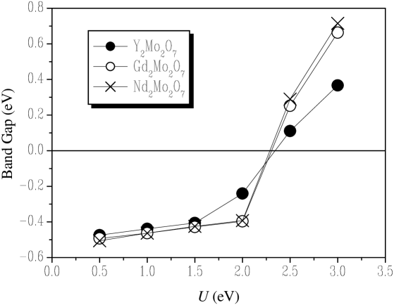
Figure 18: The band gap as a function of Coulomb $U$. For $U$$\leq$$2.0$ eV there is an overlap between bands, corresponding to the negative value of the band gap, while $U$$\geq$$2.5$ eV opens the real gap.

Typical densities of states in the insulating phase are shown in Fig. 19.

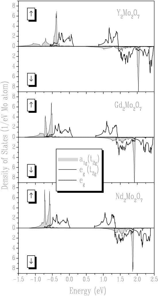
Figure 19: Distribution of the Mo($4d$) states obtained in model Hartree-Fock calculations for $U$$=$$3.0$ eV.

The insulating behavior is accompanied by the change of the orbital ordering (the distribution of the Mo($4d$) electron densities). In the metallic state, it comes exclusively from the local trigonal distortions of the oxygen octahedra and represents the alternating $a_{1g}$ orbital densities in the background of degenerate $e_{g}^{\prime}$ orbitals (Fig. 20).

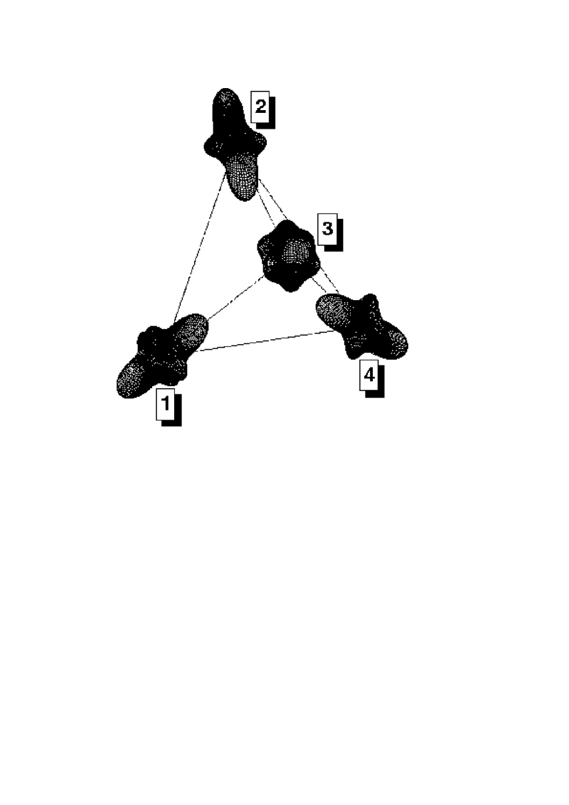
Figure 20: Orbital ordering in Nd₂Mo₂O₇ for $U$$=$$1.5$ eV.

In the insulating state, the orbital ordering is determined not only by the local trigonal distortions, but also by the form of SE interactions between NN Mo sites, and tends to minimize the energy of these interactions [8]. Two typical examples for the FM and AFM (obtained after the flip of magnetic moments at the sites 2 and 3) phases are shown in Fig. 21.

Figure 21: Orbital ordering in Y₂Mo₂O₇ for $U$$=$$3.0$ eV. Left panel: ferromagnetic phase. Two orbital sublattices are shown by black and gray colors. Right panel: antiferromagnetic phase. Two spin sublattices are show by black and gray colors.

As expected for the FM spin ordering [8], the $e_{g}^{\prime}$ orbitals tend to order ”antiferromagnetically” and form two Mo sublattices. Clearly, this orbital ordering breaks the $Fm\overline{3}d$ symmetry: if the sites belonging to the same sublattice can still be transformed to each other using the symmetry operations of the $Fm\overline{3}d$ group, the sites belonging to different sublattices – cannot. This will generally lead to the anisotropy of electronic properties, including the NN magnetic interactions. The AFM spin ordering coexists with the FM orbital ordering. It breaks the $Fm\overline{3}d$ symmetry in the spin sector, but not in the orbitals one.

Results for NN magnetic interactions are shown in Fig. 22, as a function of $U$.

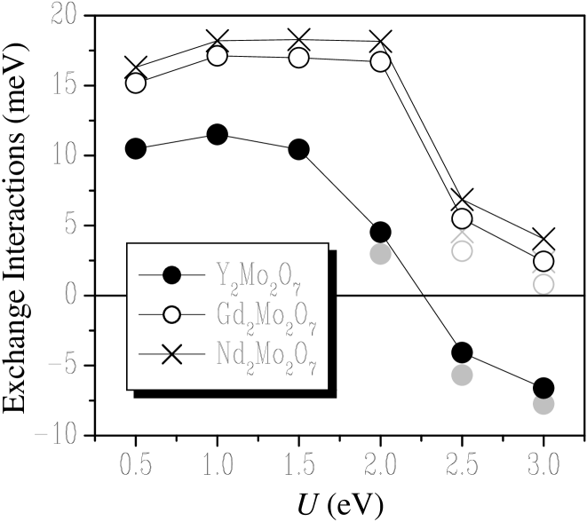
Figure 22: Nearest-neighbor exchange interactions calculated in the ferromagnetic state. The orbital ordering realized for large $U$ breaks the $Fm\overline{3}d$ symmetry, that leads to the inequality $J_{12}$$=$$J_{13}$$\neq$$J_{14}$. Two such parameters, $J_{12}$ and $J_{14}$, are shown by dark and light symbols, respectively.

We note the following.

1. $J_{\bm{\tau}\bm{\tau}^{\prime}}$, which are ferromagnetic for small $U$, exhibit a sharp drop at the point of transition into the insulating state.

2. There is a significant difference between Nd/Gd and Y based compounds: in the case of Y, the exchange parameters are almost rigidly shifted towards negative values, so that the NN coupling become antiferromagnetic in the insulating phase, while it remains ferromagnetic in the case of Nd and Gd.

The behavior can be easily understood by considering partial $a_{1g}$ and $e_{g}^{\prime}$ contributions to the NN exchange coupling, calculated after transformation to the local coordinate frame at each site of the system (Fig. 23).

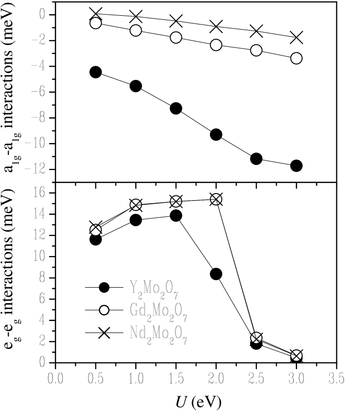
Figure 23: Contributions of $a_{1g}$ and $e_{g}^{\prime}$ orbitals (coming from the $t_{2g}$ manifold in the local coordinate frame) to the exchange constant $J_{14}$.

Large FM $e_{g}^{\prime}$-$e_{g}^{\prime}$ interaction in the metallic regime is related with the double exchange (DE) mechanism, which is the measure of the kinetic energy for the itinerant $\uparrow$-spin $e_{g}^{\prime}$ electrons. As long as the system is metallic, the DE interactions are not sensitive to the value of $U$, and the FM coupling will prevail. In the insulating state, the $e_{g}^{\prime}$ electrons are localized at the atomic orbitals. This reduces the kinetic energy and suppresses the DE interactions, that explain the sharp drop of $J_{\bm{\tau}\bm{\tau}^{\prime}}$ (Fig. 22).

The main difference between Y and Nd/Gd based compounds is related with the $a_{1g}$-$a_{1g}$ interaction. Since the $\uparrow$-spin $a_{1g}$ band is fully occupied and the $\downarrow$-spin band is empty, this interaction is antiferromagnetic due to the superexchange mechanism. Since the SE coupling is proportional to the square of the $a_{1g}$ bandwidth, this interaction will be the largest in the case of Y, that explains the AFM character of the total exchange coupling realized in this compound for large $U$.

This example clearly shows at the importance of Coulomb $U$ in the problem interatomic magnetic interactions of Mott insulators: it is absolutely indispensable in order to open the gap between occupied and unoccupied states, and suppress the FM DE interactions. Only in this case the total coupling between neighboring Mo sites can become antiferromagnetic, which is a necessary precondition for the SG behavior. On the contrary, the metallic state of Mo pyrochlores will always coexist with the ferromagnetism. Therefore, it is not right to say that the energy gap is not a ground-state property and therefore does not need to be present in the Kohn-Sham quasi-particle spectrum of the SDFT. The present example shows exactly the opposite: the energy gap may determine not only the value, but also the sign of interatomic magnetic interactions, which are the ground-state properties.

6 Concluding Remarks

In this review we tried to formulate some framework for the analysis of interatomic magnetic interactions in the transition-metal oxides and give some hints and ideas illustrating how this analysis should be generally done or at least started with on the basis of realistic electronic structure calculations. It is based on the fundamental magnetic force theorem, which allows to connect the problem of interatomic magnetic interactions in solids with the (generally auxiliary) single-particle spectrum obtained from the solution of Kohn-Sham equations in the spin-density-functional theory for the ground state.

The straightforward application of this theorem is seriously hampered by the fact that in realistic calculations, SDFT is supplemented with some approximations, which are not always adequate for TMO. Nevertheless, in many cases the electronic structure calculations can provide the basic idea or at least some useful input information for the analysis of interatomic magnetic interactions in TMO, which (perhaps with some imaginations!) can be transformed to a realistic semi-quantitative model. This point of view was illustrated for a number of popular nowadays compounds, such as CMR manganites, double perovskites Sr₂Fe$M$O₆ ($M$$=$ Mo, Re), and pyrochlores $A_{2}$Mo₂O₇ ($A$$=$ Y, Gd, and Nd).

It would be unfair to say that this strategy is universal and can be directly applied to all possible types of TMO. In some sense, we were lucky that the realistic information about the electronic structure of the considered compounds can be obtained already on the level of LSDA:

• It gives a rough idea about the competition of double exchange and superexchange interactions in CMR manganites and double perovskites.

• It allows to identify the electronic states, which are mainly responsible for the physics of Mo-pyrochlores and well separated from the rest of the spectrum, so that the next step connecting the LSDA calculations with the degenerate Hubbard model becomes basically a matter of routine.

Unfortunately, such a generalization is not always possible and there is a wide class of magnetic TMO, which still presents a very challenging problem for the first-principles electronic structure calculations. This group includes many nickelates and cuprates. These systems are especially complicated because of two reasons:

• For many of them, the standard LSDA calculations erroneously lead to the nonmagnetic ground state (the most famous example is La₂CuO₄ [77]). Therefore, it is difficult to make any conjectures basing on the LSDA.

• All these compounds are of the charge-transfer type. In this case, the semi-empirical LDA$+$$U$ calculations may not be very reliable either.

In order to proceed with the realistic description of electronic and magnetic properties of these materials, the development of new methods of electronic structure calculations, which would go beyond LSDA and get rid of several empirical features of the LDA$+$$U$ approach is a very important task.

References

- [1] Goodenough, J.B. 1955, Phys. Rev. 100, 564.
- [2] Anderson, P.W. and Hasegawa, H. 1955, Phys. Rev. 100, 675.
- [3] Kanamori, J. 1959, J. Phys. Chem. Solids 10, 87.
- [4] Anderson, P.W. 1959, Phys. Rev. 115, 2.
- [5] Oguchi, T., Terakura, K., and Williams, A.R. 1983, Phys. Rev. B 28, 6443.
- [6] Terakura, K., Oguchi, T., Williams, A.R., and Kübler, J. 1984, Phys. Rev. B 30, 4734.
- [7] De Gennes, P.-G. 1960, Phys. Rev. 118, 141.
- [8] Kugel, K. I. and Khomskii, D. I. 1982, Usp. Fiz. Nauk 136, 621.
- [9] Hohenberg, P., and Kohn, W. 1964, Phys. Rev. 136, B864; Kohn, W., and Sham, L.J. 1965, Phys. Rev. 140, A1133; von Bath, U., and Hedin, L. 1972, J. Phys. C: Solid States Phys. 5, 1629.
- [10] Gunnarsson, O. 1976, J. Phys. F: Metal Phys. 6, 587; Janak, J.F. 1977, Phys. Rev. B 16, 255.
- [11] Anisimov, V.I., Zaanen, J., and Andersen, O.K. 1991, Phys. Rev. B 44, 943.
- [12] Solovyev, I.V., Dederichs, P.H., and Anisimov, V.I. 1994, Phys. Rev. B 50, 16861.
- [13] Solovyev, I.V., Liechtenstein, A.I., and Terakura, K. 1998, Phys. Rev. Lett. 80, 5758.
- [14] Andersen, O.K. 1975, Phys. Rev. B 12, 3060; Gunnarsson, O., Jepsen, O., and Andersen, O.K. 1983, Phys. Rev. B 27, 7144; http://www.mpi-stuttgart.mpg.de/andersen/.
- [15] Talman, J.D., and Shadwick, W.F. 1976, Phys. Rev. A 14, 36.
- [16] Kotani, T., and Akai, H. 1996, Phys. Rev. B 54, 16502; Kotani, T. 1998, J. Phys.: Condens. Matter 10, 9241.
- [17] Aryasetiawan, F., and Gunnarsson, O. 1998, Rep. Prog. Phys. 61, 237.
- [18] Solovyev, I.V., and Terakura, K. 1998, Phys. Rev. B 58, 15496.
- [19] Vignale, G., and Rasolt, M. 1987, Phys. Rev. Lett. 59, 2360; Vignale, G., and Rasolt, M. 1988, Phys. Rev. B 37, 10685; Rasolt, M., and Vignale, G. 1990, Phys. Rev. Lett. 65, 1498.
- [20] Bruno, P. 2003, Phys. Rev. Lett. 90, 087205.
- [21] Liechtenstein, A.I., Katsnelson, M.I., Antropov, V.P., and Gubanov, V.A. 1987, J. Magn. Magn. Matter. 67, 65.
- [22] Nordström, L., and Singh, D.J. 1996, Phys. Rev. Lett. 76, 4420; Oda, T., Pasquarello, A., and Car, R. 1998, Phys. Rev. Lett. 80, 3622; Bylander, D.M., Niu, Q., and Kleinman L. 2000, Phys. Rev. B 61, R11875.
- [23] Halilov, S.V., Eschrig, H., Perlov, A.Y., and Oppeneer, P.M. 1998, Phys. Rev. B 58, 293.
- [24] Herring, C. 1966, in Magnetism, Vol. IV, G. Rado and H. Suhl (Ed.), Academic Press, New York, London; Sandratskii, L.M. 1986, Phys. Status Sol. B 136, 167.
- [25] Solovyev, I.V., and Terakura, K. 1999, Phys. Rev. Lett. 82, 2959.
- [26] Solovyev, I.V., and Terakura, K. 2003, in Electronic Structure and Magnetism of Complex Materials, D. J. Singh and D. A. Papaconstantopoulos (Eds.), Springer, Berlin.
- [27] Zaanen, J., and Sawatzky, G.A. 1987, Can. J. Phys. 65, 1262.
- [28] Blackman, J.A., and Elliott, R.J. 1969, J. Phys. C: Solid States Phys. 2, 1670; Bulaevskii, L.N, and Panyukov, S.V. 1986, JETP Lett. 43, 240; Lang, P., Nordström, L., Wildberger, K., Zeller, R., Dederichs, P.H., and Hoshino, T. 1996, Phys. Rev. B 53, 9092; Levy, P.M., Maekawa, S., and Bruno, P. 1998, Phys. Rev. B 58, 5588.
- [29] Solovyev, I.V. 1999, Phys. Rev. B 60, 8550.
- [30] Lines, M.E., and Jones, E.D. 1965, Phys. Rev. 139, A1313; Kohgi, M., Ishikawa, Y., and Endoh, Y. 1972, Solid State Commun. 11, 391; Pepy G. 1974, J. Phys. Chem. Solids 35, 433.
- [31] Held, K., Keller, G., Eyert, V., Vollhardt, D., and Anisimov, V.I. 2001, Phys. Rev. Lett. 86, 5345; Savrasov, S.Y. and Kotliar, G. 2003, Phys. Rev. Lett. 90, 056401.
- [32] Kuwahara, H., Okuda, T., Tomioka, Y., Asamitsu, A., and Tokura, Y. 1998, in Science and Technology of Magnetic Oxides, M. Hundley, J. Nickel, R. Ramesh, and Y. Tokura (Eds.). MRS Symposia Proceedings No. 494, Materials Research Society, Pittsburg.
- [33] Imada, M., Fujimori, A., and Tokura, Y. 1998, Rev. Mod. Phys. 70, 1039.
- [34] Tokura, Y. (Ed.) 2000, Colossal Magnetoresistive Oxides, Gordon and Breach Science Publishers, Tokyo.
- [35] Dagotto, E., Hotta, T., and Moreo, A. 2001, Phys. Rep. 344, 1.
- [36] Mahadevan, P., Shanthi, N., and Sarma, D.D. 1997, J. Phys.: Condens. Matter 9, 3129; Papaconstantopoulos, D.A., and Pickett, W.E. 1998, Phys. Rev. B 57, 12751.
- [37] van den Brink, J., and Khomskii, D. 1999, Phys. Rev. Lett. 82, 1016.
- [38] Solovyev, I.V., and Terakura, K. 2001, Phys. Rev. B 63, 174425.
- [39] Solovyev, I.V., and Terakura, K. 1999, Phys. Rev. Lett. 83, 2825; Solovyev, I.V. 2001, Phys. Rev. B 63, 174406.
- [40] Kino, H., Aryasetiawan, F., Miyake, T., Solovyev, I., Ohno, T., and Terakura, K. 2003, Physica B (in press).
- [41] Lee, J., Yu, J., and Terakura, K. 1998, J. Korean Phys. Soc. 33, S55.
- [42] Murakami, Y., Kawada, H., Kawata, H., Tanaka, M., Arima, T., Moritomo, Y., and Tokura, Y. 1998, Phys. Rev. Lett. 80, 1932.
- [43] Andersen, O.K., Liechtenstein, A.I., Jepsen, O., and Paulsen, F. 1995, J. Phys. Chem. Solids 56, 1573.
- [44] Slater, J.C., and Koster, G.F. 1954, Phys. Rev. 94, 1498.
- [45] Müller-Hartmann, E., and Dagotto, E. 1996, Phys. Rev. B 54, R6819.
- [46] Solovyev, I.V. 2003, Phys. Rev. B 57, 014412.
- [47] Maezono, R., Ishihara, S., and Nagaosa, N. 1998, Phys. Rev. B 58, 11583.
- [48] Fang, Z., Solovyev, I.V., and Terakura, K. 2000, Phys. Rev. Lett. 84, 3172.
- [49] Shen, S.Q. 2001, Phys. Rev. Lett. 86, 5842.
- [50] Yunoki, S., Hotta, T., and Dagotto, E. 2000, Phys. Rev. Lett. 84, 3714.
- [51] Hotta, T., Takada, Y., and Koizumi, H. 1998, Int. J. Mod. Phys. B 12, 3437.
- [52] Kuwahara, H., Okuda, T., Tomioka, Y., Asamitsu, A., and Tokura, Y. 1999, Phys. Rev. Lett. 82, 4316.
- [53] Moreo, A., Mayr, M., Feiguin, A., Yunoki, S., and Dagotto, E. 2000: Phys. Rev. Lett. 84, 5568; Mayr, M., Moreo, A., Vergés, J.A., Arispe, J., Feiguin, A., and Dagotto, E. 2001, Phys. Rev. Lett. 86, 135.
- [54] Nagaev, E.L. 1996, Physics-Uspekhi 39, 781; and references therein.
- [55] Solovyev, I.V. 2003, e-print cond-mat/0212608.
- [56] Chen, C.H., and Cheong, S-W. 1996, Phys. Rev. Lett. 76, 4042; Chen, C.H., Mori. S, and Cheong, S-W. 1999, Phys. Rev. Lett. 83, 4792; Jirák, Z., Damai, F., Hervieu, M., Martin, C., Raveau, B., André, G., and Bourée, F. 2000, Phys. Rev. B 61, 1181; Kajimoto, R., Yoshizawa, H., Tomioka, Y., and Tokura, Y. 2001, Phys. Rev. B 63, 212407.
- [57] Arima, T., Akahoshi, D., Oikawa, K., Kamiyama, T., Uchida, M., Matsui, Y., and Tokura, Y. 2002, Phys. Rev. B 66, 140408.
- [58] Hwang, H.Y., Dai, P., Cheong, S-W., Aeppli, G., Tennant, D.A., and Mook, H.A. 1998, Phys. Rev. Lett. 80, 1316; Fernandez-Baca, J.A., Dai, P., Hwang, H.Y., Kloc, C., and Cheong, S-W. 1998, Phys. Rev. Lett. 80, 4012.
- [59] Motome, Y., and Furukawa, N. 2002, J. Phys. Soc. Jpn. 71, 2002.
- [60] Kobayashi, K.-I., Kimura, T., Sawada, H., Terakura, K., and Tokura, Y. 1998, Nature (London) 395, 677; Kobayashi, K.-I., Kimura, T., Tomioka, Y., Sawada, H., Terakura, K., and Tokura, Y. 1999, Phys. Rev. B 59, 11159.
- [61] Tomioka, Y., Okuda, T., Okimoto, Y., Kumai, R., Kobayashi, K.-I. and Tokura, Y. 2000, Phys. Rev. B 61, 422.
- [62] Solovyev, I.V. 2002, Phys. Rev. B 65, 144446.
- [63] Kanamori, J. and Terakura, K. 2001, J. Phys. Soc. Jpn. 70, 1433.
- [64] Kobayashi, K.-I., Okuda, T., Tomioka, Y., Kimura, T., and Tokura, Y. 2000, J. Magn. Magn. Matter. 218, 17.
- [65] Singh, D.J. 2003, in Electronic Structure and Magnetism of Complex Materials, D.J. Singh and D.A. Papaconstantopoulos (Eds.), Springer, Berlin.
- [66] Katsufuji, T., Hwang, H.Y., and Cheong, S-W. 2000, Phys. Rev. Lett. 84, 1998.
- [67] Moritomo, Y., Xu, Sh., Machida, A., Katsufuji, T., Nishibori, E., Takata, M., Sakata, M., and Cheong, S-W. 2001, Phys. Rev. B 63, 144425.
- [68] Taguchi, Y., Ohgushi, K., and Tokura, Y. 2002, Phys. Rev. B 65, 115102.
- [69] Iikubo, S., Yoshii, S., Kageyama, T., Oda, K., Kondo, Y., Murata, K., and Sato, M. 2001, J. Phys. Soc. Jpn. 70, 212.
- [70] Reimers, J.N., Greedan, J.E., and Sato, M. 1988, J. Solid State Chem. 72, 390; Gardner, J.S., Gaulin, B.D., Lee, S.-H., Broholm, C., Raju, N.P., and Greedan, J.E. 1999, Phys. Rev. Lett. 83, 211.
- [71] Reimers, J.N. 1992, Phys. Rev. B 45, 7287.
- [72] Booth, C.H., Gardner, J.S., Kwei, G.H., Heffner, R.H., Bridges, F., and Subramanian, M.A. 2000, Phys. Rev. B 62, R755; Keren, A., and Gardner, J.S. 2001, Phys. Rev. Lett. 87, 177201.
- [73] Singh, D.J. 1996, J. Appl. Phys. 79, 4818.
- [74] Anisimov, V.I., Korotin, M.A., Zölfl, M., Pruschke, T., Le Hur, K., and Rice, T.M. 1998, Phys. Rev. Lett. 80, 5758.
- [75] Solovyev, I.V. 2003, Phys. Rev. B 97, 174406.
- [76] Solovyev, I., Hamada, N., and Terakura, K. 1996, Phys. Rev. B 53, 7158.
- [77] Pickett, W.E. 1989, Rev. Mod. Phys. 61, 433.