Density of states of a binary Lennard-Jones Glass

Abstract

We calculate the density of states of a binary Lennard-Jones glass using a recently proposed Monte Carlo algorithm. Unlike traditional molecular simulation approaches, the algorithm samples distinct configurations according to self-consistent estimates of the density of states, thereby giving rise to uniform internal-energy histograms. The method is applied to simulate the equilibrium, low-temperature thermodynamic properties of a widely studied glass former consisting of a binary mixture of Lennard-Jones particles. We show how a density-of-states algorithm can be combined with particle identity swaps and configurational bias techniques to study that system. Results are presented for the energy and entropy below the mode coupling temperature.

I Introduction

The transition from a liquid to an amorphous solid that sometimes occurs upon cooling remains one of the largely unresolved problems of statistical physics Ediger et al. (1996); Debenedetti and Stillinger (2001). At the experimental level, the so-called glass transition is generally associated with a sharp increase in the characteristic relaxation times of the system, and a concomitant departure of laboratory measurements from equilibrium. At the theoretical level, it has been proposed that the transition from a liquid to a glassy state is triggered by an underlying thermodynamic (equilibrium) transition Mezard and Parisi (1999); in that view, an “ideal” glass transition is believed to occur at the so-called Kauzmann temperature, $T_{K}$. At $T_{K}$, it is proposed that only one minimum-energy basin of attraction is accessible to the system. One of the first arguments of this type is due to Gibbs and diMarzio Gibbs and DiMarzio (1958), but more recent studies using replica methods have yielded evidence in support of such a transition in Lennard-Jones glass formers Mezard and Parisi (1999); Coluzzi et al. (2000a); Grigera and Parisi (2001). These observations have been called into question by experimental data and recent results of simulations of polydisperse hard-core disks, which have failed to detect any evidence of a thermodynamic transition up to extremely high packing fractions Santen and Krauth (2000). One of the questions that arises is therefore whether the discrepancies between the reported simulated behavior of hard-disk and soft-sphere systems is due to fundamental differences in the models, or whether they are a consequence of inappropriate sampling at low temperatures and high densities.

Different, alternative theoretical considerations have attempted to establish a connection between glass transition phenomena and the rapid increase in relaxation times that arises in the vicinity of a theoretical critical temperature (the so-called “mode-coupling” temperature, $T_{MCT}$), thereby giving rise to a “kinetic” or “dynamic” transition Götze and Sjögren (1992). In recent years, both viewpoints have received some support from molecular simulations. Many of these simulations have been conducted in the context of models introduced by Stillinger and Weber and by Kob and Andersen  Kob and Andersen (1995); such models have been employed in a number of studies that have helped shape our current views about the glass transition Sastry et al. (1998); Sciortino et al. (1999); Donati et al. (1999); Coluzzi et al. (2000a, b); Yamamoto and Kob (2000). The particular model considered here consists of a binary mixture of Lennard-Jones particles, with composition 80% $A$ and 20% $B$. A total of 250 particles is employed in our calculations. The interaction parameters between particles of species $A$ and $B$ are $\epsilon_{AA}=1.0$ and $\sigma_{AA}=1.0$, $\epsilon_{BB}=0.5$ and $\sigma_{BB}=0.88$, and $\epsilon_{AB}=1.5$ and $\sigma_{AB}=0.8$. The density is $1.204\sigma_{AA}^{-3}$. Recently, a crystal structure at extremely low energies has been reported for a variant of this system Middleton et al. (2001).

High-precision data are available for the thermodynamic properties of this model at intermediate to high temperatures Kob and Andersen (1995); Yamamoto and Kob (2000); Coluzzi et al. (2000b). A series of careful simulations have placed the mode coupling temperature at $T_{MCT}=0.435$ and the Kauzmann temperature somewhere in the range $T_{K}=0.26-0.31$ Yamamoto and Kob (2000); Sciortino et al. (1999); Coluzzi et al. (2000b). Note, however, that literature studies have generally avoided direct simulations below $T_{MCT}$; available estimates of $T_{K}$ have been produced after making several assumptions regarding the potential energy landscape and by extrapolation (to low temperatures) of liquid-state data generated at higher temperatures (above $T_{MCT}$). An exception is provided by a recent report for a related model Grigera and Parisi (2001), where simulations of small systems, directly at low temperatures, suggest that an anomaly in the heat capacity $c_{v}$ arises at $T_{K}$; $c_{v}$ is reported to increase with decreasing temperature, and to exhibit a sharp drop at $T_{K}$. The drop becomes more pronounced as the system size is increased.

Simulations near a glass transition are notoriously difficult, and their results must be considered with caution. On the one hand, the relevant time scales below $T_{MCT}$ are too long to be sampled by conventional molecular dynamics simulations. Monte Carlo techniques, on the other hand, have been used only rarely to simulate glass formers; furthermore, it has been difficult to establish to what extent available studies have succeeded in sampling relevant regions of phase space, particularly at low temperatures and elevated densities. In this work, we use a novel Monte Carlo sampling technique to arrive at direct estimates of the thermodynamic properties of a model glass former down to temperatures well below $T_{MCT}$.

II Simulation Methods

Recently, Wang and Landau have proposed an iterative method to estimate the density of states of a Potts lattice system from a Monte Carlo simulation Wang and Landau (2001a, b). The random-walk algorithm is based on the idea of entropic sampling, with a self-consistent update of the density of states. It has proven to be remarkably efficient for lattice systems, simple liquids Yan et al. (2002), proteins Rathore and de Pablo (2002); Rathore et al. (2003), and liquid crystals Kim et al. (2002); it is tempting to apply it in the context of a glass-forming liquid. In this contribution we combine it with biased sampling techniques, and we use it to generate direct estimates of the density of states of the glass-former described above.

In a conventional canonical-ensemble simulation, different states of the system are visited with probability $\Omega(E)e^{-E/k_{B}T}$, where $\Omega(E)$ is the density of states (or degeneracy) of the system, $k_{B}$ is Boltzmann’s constant, and $T$ is the temperature. In contrast, in the random-walk scheme adopted here, the density of states $\Omega(E)$ is estimated directly by producing a uniform, or “flat” histogram of energies, i.e. by coercing the system to visit all energy states with equal probability. In this study we have chosen to maintain a constant density and constant number of particles; extensions to other physical ensembles and to expanded ensembles have also been pursued recently Yan et al. (2002); Kim et al. (2002); Calvo (2002). Trial moves are generated by means of simple translations of the particles and by identity interchanges Grigera and Parisi (2001). The acceptance of such interchanges is enhanced using configurational bias. The resulting trial configurations are accepted with probability Jain and de Pablo (2002)

$$p=\text{min}\Big{\{}1,\frac{W^{R}_{new}\Omega^{\prime}(E_{old})}{W^{R}_{old}\Omega^{\prime}(E_{new})}\Big{\}}$$ (1)

where the prime indicates that this is a transient, momentary “best estimate” of the density of states. Biased moves are performed according to a Rosenbluth type algorithm; $W^{R}$ is the Rosenbluth weight of the corresponding state. In the original version by Wang and Landau $W^{R}$ was set to unity for all states. The configurational bias identity swap consists of the following steps: First a pair on unlike particles is chosen at random. After direct interchange of their positions, the smaller particle $B$ will fit in the cavity formerly occupied by the larger particle $A$. The opposite is only seldom true, thereby leading to negligible acceptance rates at low energies and high densities. In order to enhance the acceptance rate, $N_{CCB}=12-100$ trial positions are explored for the $B$ particle around the position formerly occupied by the $A$ particle. We then apply configurational bias ideas to these $N_{CCB}$ positions. There are now two possible ways to calculate the Rosenbluth factors. In the first of these, the energy of the states can be used directly (as is done in standard configurational bias Monte Carlo) de Pablo et al. (1992); Frenkel and Smit (1996). To this end, a fictitious temperature $T_{F}$ is introduced for calculation of the Rosenbluth factor $W^{R}_{i}$ for state $i$

$$W^{R}_{i}=\frac{\exp(-\beta_{F}E_{i})}{\sum_{j}\exp(-\beta_{F}E_{j})}.$$ (2)

Note that this fictitious temperature is not the temperature of the system, although in conventional configurational bias simulations it is set to the system temperature. Alternatively, one can avoid using a fictitious temperature by calculating a set of $W_{R}$ using the density of states itself as a bias.

$$W^{R}_{i}=\frac{\Omega_{i}}{\sum_{j}\Omega_{j}}.$$ (3)

Both variants (using $T_{F}=0.5-1$) behave similarly. The acceptance rate is extremely small (it drops to less than $10^{-6}$ as the effective temperature approaches $T_{g}$), but it is sufficient to perform simulations over extended amounts of computer time. The effective temperature $T_{\text{eff}}$ of a state with energy $E$ is defined as the temperature where $\langle E_{pot}\rangle_{T_{\text{eff}}}=E$.

The density of states is not known á priori; it is initially set to unity throughout the entire energy range. The calculations begin by defining an energy range in which to determine $\Omega(E)$. Whenever an energy state $E$ is visited, the density of states $\Omega^{\prime}(E)$ corresponding to that energy is multiplied by a constant $f$, i.e. $\Omega^{\prime}(E)\rightarrow f\Omega^{\prime}(E)$. Since the density of states varies over many orders of magnitude, it is convenient to work with its logarithm, which corresponds to the entropy as a function of energy $S(E)=-k_{B}\ln\Omega(E)$. The entropy is updated by adding a constant $\ln f$.

A histogram of energies $h(E)$ is also constructed and updated after every trial move. The density of states is updated continuously throughout the simulation, until the recorded energy histogram $h(E)$ is sufficiently flat. Note that in actual practice it is not possible to generate a perfectly flat histogram; in this work, flatness is considered to be attained if the minimum of $h(E)$ is at least 0.9 times the average value $\overline{h(E)}$. Having reached a “flat-histogram” condition, the simulation sequence is repeated: the energy histogram is erased, and the new value of $\ln f$ is set to half the “old” value. Note that this choice is arbitrary, and any monotonically decreasing function should work. The initial value of $\ln f$ was set to unity, and the final value was $\ln f=10^{-5}$, which corresponds to 18 iterations. The factor $\ln f$ controls the convergence of $\Omega^{\prime}(E)$ to the true value, $\Omega(E)$; as $\ln f$ decreases (i.e. as the simulation proceeds) the calculations per iteration become increasingly long.

To improve efficiency, it is useful to conduct multiple simulations in overlapping energy ranges. These ranges must be relatively narrow; otherwise, given the rapidly varying nature of $\Omega(E)$, the calculations can be prohibitively long. The energy ranges employed here correspond to $E_{\text{max}}-E_{\text{min}}=200-400$, or $(E/N)_{\text{max}}-(E/N)_{\text{min}}=1.0-2.0$ per particle. In order to generate $\Omega(E)$ over a wide energy range, neighboring energy windows were constructed in such a way as to overlap by half their width; every region of the energy axis is covered by at least two independent simulations. Two sets of independent simulations with energy windows of 200 or 400 units wide were pursued here. At low energies, convergence was only possible with relatively narrow energy ranges. The lowest energy range employed here starts at $E=-1860$ ($E/N=-7.44$), which is slightly above the range of estimated intrinsic energies for this system Sciortino et al. (1999) and well above the crystal energies Middleton et al. (2001). After the density of states converged to within a certain accuracy the update of $\Omega(E)$ was stopped. A simple multicanonical run was then employed, where the inverse of the DOS was used as the weighting function. After a long run (25 million steps) the density of states was corrected by adding the logarithm of the final histogram. This was necessary as we did not run the simulations to update factors of $f=\exp(10^{-8})$ as in the original work by Wang and Landau Wang and Landau (2001a, b). It was verified during the course of the simulation that the logarithmic energy histograms kept increasing homogeneously (Figure 1a). This was monitored by observing that the logarithms of the histograms taken at different points in time during the final run are filled homogeneously. In a theoretically ideal situation, the different (logarithmic) histograms would be parallel to each other. However, the stochastic nature of the simulation leads to departures from parallel behavior. Nonetheless, we see that the system never gets “trapped” in a certain energy region without visiting the others. This ensures that the system readily moves back and forth between high and low energy regions of phase space, which is analogous to moving through temperatures in other types of simulations. In the case of continuous degrees of freedom this additional monitoring is important.

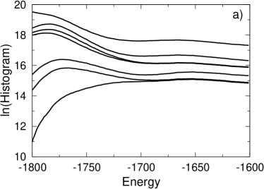
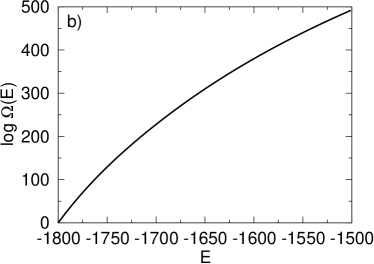
Figure 1: a) Logarithm of the energy histogram in the final run without updating the weights in different stages of the simulation. The curves are parallel to each other. b) Logarithm of the density of states over the decisive energy range [-1800,-1500].

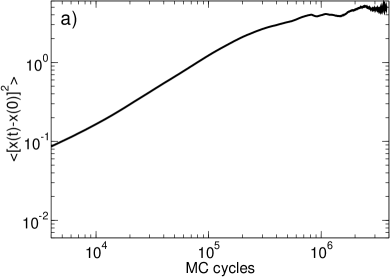
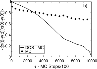
Figure 2: a) Average mean-squared displacement in the final multicanonical run (see text). The length of the simulation box is 5.96. The mean-squared displacement is calculated in the original box so it apparently levels off approaching the box size. b) Position autocorrelation function from Monte Carlo simulations and from molecular dynamics at $T=0.45$.

In order to provide an assessment of the correlation time of the random-walk method, the mean squared displacement of the particles was also measured. It is observed that in the final multicanonical run approximately 2 million cycles are necessary for the mean-squared displacement to be comparable to the box length (in one MC cycle each particle is moved once). The simulations presented here are at least 10 times that length (cf. Figure 2). A positional autocorrelation function can be defined as

$$C_{pos}(t)=\langle(\vec{x}_{i}(t_{0}+t)-\vec{x}_{j}(t_{0}+t))(\vec{x}_{i}(t_{0})-\vec{x}_{j}(t_{0}))\rangle_{i,j,t_{0}}.$$ (4)

This measure of relaxation is more stringent than the mean-square displacement as it eliminates the possibility that blocks of particles might be moving together without too much mutual rearrangement. This function decays to zero within the simulation lengths considered here. Figure 2 also compares this function to that obtained from molecular dynamics runs at $T=0.45$. To the best of our knowledge, the longest runs reported in the literature Yamamoto and Kob (2000) for the system considered here have lasted $10^{5}\tau$ ($\tau$ is the usual dimensionless Lennard-Jones time, which typically corresponds to 100 timesteps). In $10^{5}\tau$, this function decays to about 70% of its initial value. The scale employed in Figure 2 assumes that the computational requirements for one MD timestep are comparable to those of one MC cycle.

In regions of overlap, the density of states corresponding to each window can only differ by a constant, which depends on the (arbitrary) number of histogram entries. The density of states over the entire energy range of interest is constructed by shifting local estimates of $\ln\Omega(E)$ (corresponding to individual windows) until they coincide, in the middle of the overlap region.

The global density of states is therefore known to within a constant. Since internal energies are known exactly, the excess free energy of the system can be calculated as a function of $T$ according to

$$\beta\langle F(T)^{\text{ex}}\rangle=-\ln\;\sum_{E}\Omega(E)\;e^{-\beta E},$$ (5)

where the brackets denote an ensemble average and where $\beta=1/k_{B}T$. Similarly, the average internal energy of the system is given by

$$\beta\langle E(T)^{\rm ex}\rangle=\frac{\sum_{E}E\;\Omega(E)\;e^{-\beta E}}{\sum_{E}\Omega(E)\;e^{-\beta E}},$$ (6)

and the entropy can simply be determined from $\langle S\rangle=(\langle U\rangle-\langle F\rangle)/T$. Note that the total entropy also comprises an ideal-mixing contribution of the form $1-\ln\rho-x_{A}\ln x_{A}-x_{B}\ln x_{B}$, where $x_{A}$ represents the mole fraction of species $A$ in the mixture. There is a second way to access properties, directly from the microcanonical ensemble. For example, the internal energy as a function of temperature can be derived by differentiation of the entropy (i.e. $k_{B}\ln\Omega(E)$) with respect to energy and and subsequent inversion of that curve. This relies on the microcanonical definition of temperature, namely $T=\langle\frac{dS}{dE}\rangle^{-1}$.

III Results

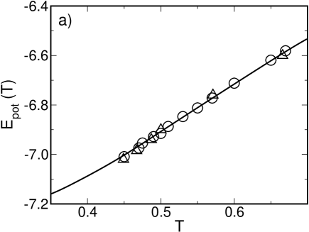
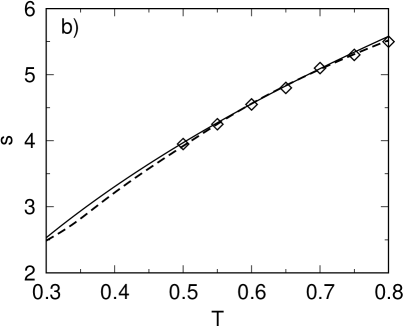
Figure 3: a) Energy per particle calculated by canonical MC (circles), and density of states (solid line). Triangles are literature values Yamamoto and Kob (2000). b) Entropy per particle. The dashed line shows the total entropy (excess plus ideal) determined from the density of states. The symbols are literature results Coluzzi et al. (2000b). The solid line is a fit to the literature data of the form $S=10.27*T^{0.4}-3.81$.

Figure 3a shows the average internal energy of the binary Lennard-Jones glass former. Results by Yamamoto et al. Yamamoto and Kob (2000) obtained by replica exchange Molecular Dynamics are also shown in that figure. The agreement between the two sets of data is quantitative. At temperatures below $T_{MCT}$ we have performed additional, extensive simulations using biased-sampling ideas and parallel-tempering techniques. More specifically, the algorithms developed for these additional calculations use two-dimensional parallel tempering in temperature Marinari and Parisi (1992); Tesi et al. (1996); Hansmann (1997); Wu and Deem (1999); Yan and de Pablo (1999) and Hamiltonian Bunker and Dünweg (2001), and identity swap moves Grigera and Parisi (2001) augmented with configurational bias sampling de Pablo et al. (1992). These techniques permit simulations at temperatures below $T_{MCT}$, but become increasingly sluggish as temperature is decreased. Still, the agreement for the energy generated by those simulations and the Density of States technique is also good, thereby providing further consistency tests for the results presented here.

The entropy of the binary Lennard-Jones glass former is shown in Fig. 3b as a function of temperature. The points in the figure represent literature data generated by thermodynamic integration Coluzzi et al. (2000b); the entropies simulated in this work have been shifted by a constant to make them coincide with those data in the range $0.5<T<0.8$. The agreement between our results and those of Coluzzi et al. is excellent. In order to arrive at an estimate of the Kauzmann temperature, these authors extrapolate the liquid phase entropy below $T=0.5$ using an expression of the form $S=aT^{0.4}+b$. We find that such a functional form is in good agreement with our simulations; at lower temperatures, however, minor but systematic departures from our results are observed. This would be indicative of a slightly higher Kauzmann temperature than that reported in the literature ($T_{K}\approx 0.3$) Sciortino et al. (1999); Coluzzi et al. (2000b), as the simulated entropy decays more rapidly than that anticipated by extrapolation.

IV Discussion

The density of states as a function of temperature does not show any unexpected behavior over the entire energy region considered in this work. Its logarithm simply becomes steeper with decreasing energy (see Figure 1b), reflecting the fact that the number of accessible states becomes smaller. The system could conceivably undergo a gas-liquid (or gas-glass) phase transition at very low temperatures. To address this point we have also determined the pressure. Our results suggest that such a transition can occur at $T\approx 0.2$, where the pressure of the glass becomes equal to that of the gas $p\approx 0$. For the same system (but without cutoff corrections), Coluzzi and Parisi estimated such a transition at $T\approx 0.3$. The occurrence of a demixing transition can be ruled out by the shape of the various pair distribution functions (not shown here), which remain qualitatively unchanged in the range $0.2<T<0.6$. A very similar system has been found to crystallize at such low temperatures Middleton et al. (2001). However, crystallization is avoided in our calculations by restricting the simulations to energy ranges above those of the crystal. Moreover, crystallization has only been found in constant pressure simulations. The volume is kept constant in this work, thereby leading to frustration of crystallization.

The results presented in this work suggest that a Monte Carlo technique based on the concept of entropic sampling is capable of generating high-accuracy estimates of the equilibrium density of states of a binary Lennard-Jones glass former, down to temperatures below the mode coupling temperature, a region of temperature that previous studies of glass-forming liquids have avoided. With further refinement of the algorithm discussed in this work Yan and de Pablo (2003), we expect that reliable simulations in the near vicinity of the reported Kauzmann temperature will become possible.

References

- Ediger et al. (1996) M. D. Ediger, C. A. Angell, and S. R. Nagel, J Phys Chem 100(31), 13200 (1996).
- Debenedetti and Stillinger (2001) P. G. Debenedetti and F. H. Stillinger, Nature 410(6825), 259 (2001).
- Mezard and Parisi (1999) M. Mezard and G. Parisi, Phys Rev Lett 82(4), 747 (1999).
- Gibbs and DiMarzio (1958) J. H. Gibbs and E. A. DiMarzio, J Chem Phys 28(3), 373 (1958).
- Coluzzi et al. (2000a) B. Coluzzi, G. Parisi, and P. Verrocchio, Phys Rev Lett 84(2), 306 (2000a).
- Grigera and Parisi (2001) T. S. Grigera and G. Parisi, Phys Rev E 63, 045102(R) (2001).
- Santen and Krauth (2000) L. Santen and W. Krauth, Nature 405(6786), 550 (2000).
- Götze and Sjögren (1992) W. Götze and L. Sjögren, Rep Prog Phys 55(3), 241 (1992).
- Kob and Andersen (1995) W. Kob and H. C. Andersen, Phys. Rev. E 51(5), 4626 (1995).
- Sastry et al. (1998) S. Sastry, P. G. Debenedetti, and F. H. Stillinger, Nature 393(6685), 554 (1998).
- Sciortino et al. (1999) F. Sciortino, W. Kob, and P. Tartaglia, Phys. Rev. Lett. 83(16), 3214 (1999).
- Donati et al. (1999) C. Donati, S. C. Glotzer, P. H. Poole, W. Kob, and S. J. Plimpton, Phys Rev E 60(3), 3107 (1999).
- Coluzzi et al. (2000b) B. Coluzzi, G. Parisi, and P. Verocchio, J Chem Phys 112(6), 2933 (2000b).
- Yamamoto and Kob (2000) R. Yamamoto and W. Kob, Phys Rev E 61(5), 5473 (2000).
- Middleton et al. (2001) T. F. Middleton, J. Hernandez-Rojas, P. N. Mortenson, and D. J. Wales, Phys Rev B 64(18), 184201 (2001).
- Wang and Landau (2001a) F. Wang and D. P. Landau, Phys. Rev. Lett. 86(10), 2050 (2001a).
- Wang and Landau (2001b) F. Wang and D. P. Landau, Phys Rev E 64(5), 056101 (2001b).
- Yan et al. (2002) Q. Yan, R. Faller, and J. J. de Pablo, J Chem Phys 116(20), 8745 (2002).
- Rathore and de Pablo (2002) N. Rathore and J. J. de Pablo, J Chem Phys 116(16), 7225 (2002).
- Rathore et al. (2003) N. Rathore, T. A. Knotts, and J. J. de Pablo, J Chem Phys 118(9), 4285 (2003).
- Kim et al. (2002) E. B. Kim, R. Faller, Q. Yan, N. L. Abbott, and J. J. de Pablo, J Chem Phys 117(16), 7781 (2002).
- Calvo (2002) F. Calvo, Mol Phys 100(21), 3421 (2002).
- Jain and de Pablo (2002) T. S. Jain and J. J. de Pablo, J Chem Phys 116(16), 7238 (2002).
- de Pablo et al. (1992) J. J. de Pablo, M. Laso, and U. W. Suter, J. Chem. Phys. 96(3), 2395 (1992).
- Frenkel and Smit (1996) D. Frenkel and B. Smit, Understanding Molecular Simulation: From Basic Algorithms to Applications (Academic Press, San Diego, CA, 1996).
- Marinari and Parisi (1992) E. Marinari and G. Parisi, Europhys. Letters 19(6), 451 (1992).
- Tesi et al. (1996) M. C. Tesi, E. J. J. van Rensburg, E. Orlandini, and S. G. Whittington, J Stat. Phys. 82(1-2), 155 (1996).
- Hansmann (1997) U. H. E. Hansmann, Chem. Phys. Lett. 281(1-3), 140 (1997).
- Wu and Deem (1999) M. G. Wu and M. W. Deem, Mol. Phys. 97(4), 559 (1999).
- Yan and de Pablo (1999) Q. Yan and J. J. de Pablo, J. Chem. Phys. 111(21), 9509 (1999).
- Bunker and Dünweg (2001) A. Bunker and B. Dünweg, Phys. Rev. E 63, 016701 (2001).
- Yan and de Pablo (2003) Q. Yan and J. J. de Pablo, Phys Rev Lett 90(3), 035701(1 (2003).