Ensemble dependence in the Random transverse-field Ising chain.

Abstract

In a disordered system one can either consider a microcanonical ensemble, where there is a precise constraint on the random variables, or a canonical ensemble where the variables are chosen according to a distribution without constraints. We address the question as to whether critical exponents in these two cases can differ through a detailed study of the random transverse-field Ising chain. We find that the exponents are the same in both ensembles, though some critical amplitudes vanish in the microcanonical ensemble for correlations which span the whole system and are particularly sensitive to the constraint. This can appear as a different exponent. We expect that this apparent dependence of exponents on ensemble is related to the integrability of the model, and would not occur in non-integrable models.

I Introduction

In the study of the critical behavior of disordered systems, it is usual to pick the random variables from some distribution. This allows sample-to-sample fluctuations in the sum of the interactions (e.g. nearest neighbor) of order $\sqrt{N}$. We will call this the canonical ensemble of disorder, by analogy with the canonical ensemble of statistical mechanics which allows fluctuations in the energy. It is sometimes of interest to complete this analogy and define a microcanonical ensemble of the disorder in which there is a strict constraint, for example by fixing exactly the sum of the (e.g. nearest neighbor) interactions in each sample. Our experience from conventional statistical mechanics tells us that in the thermodynamic limit the choice of ensembles does not matter but it is not very clear that this is also true for random systems, especially for the case of quantum phase transitions.

In this paper we will study the simplest disordered model with a quantum phase transition, the random transverse-field Ising chain (RTFIC) Fisher (1995); Fisher and Young (1998) with the Hamiltonian:

$${\cal H}=-\sum_{i=1}^{L-1}J_{i}\sigma^{z}_{i}\sigma^{z}_{i+1}-\sum_{i=1}^{L}h_{i}\sigma^{x}_{i}.$$ (1)

where $J_{i}>0$ and $h_{i}>0$ are random variables chosen from distributions $\rho(h)$ and $\pi(J)$ with averages $[\ln h]_{\rm av},~{}[\ln J]_{\rm av}$ and variances ${\rm var}(\ln h),~{}{\rm var}(\ln J)$. We use free boundary conditions, so the sum for the $J_{i}$ stops at $L-1$.

Let us define the two ensembles, microcanonical and canonical, precisely for this model. For the canonical ensemble the $h_{i}$ and $J_{i}$ are chosen randomly. A parameter which characterizes the deviation from criticality is $\bar{\delta}$ where

$$\bar{\delta}=\frac{[\ln h]_{\rm av}-[\ln J]_{\rm av}}{{\rm var}(\ln h)+{\rm var}(\ln J)},$$ (2)

For the microcanonical ensemble we constrain the $h_{i}$ and $J_{i}$ such that the parameter

$$\delta=\frac{1}{L-1}\frac{\sum_{i=1}^{L}\ln h_{i}-\sum_{i=1}^{L-1}\ln J_{i}-[\ln h]_{\rm av}}{{\rm var}(\ln h)+{\rm var}(\ln J)}$$ (3)

is set to a prescribed value for each sample. The last term in the numerator, which is not necessary to get the asymptotic behavior, corrects for there being one more $h_{i}$ than $J_{i}$ with free boundary conditions. It ensures that $\bar{\delta}=[\delta]_{\rm av}$ even for a finite system. In the canonical ensemble, the fluctuations in $\delta$ from sample to sample are $O(1/\sqrt{L})$. It is known that a phase transition occurs in this model at $\bar{\delta}=0$. All our numerical results in the paper will be at the critical point.

Pazmandi et al.Pazmandi et al. (1997) have argued that it is precisely the $O(1/\sqrt{L})$ fluctuations which lead to the bound on the finite size correlation length exponentChayes et al. (1986, 1989); Harris (1974) $\nu\geq 2/d$. Further, they argue that exponents in the microcanonical ensemble need not satisfy this bound. In addition, Igloi and RiegerIgloi and Rieger (1998) claim that the exponents of the RTFIC can depend on the choice of ensemble. In this paper our main goal is to investigate these claims through a detailed study of the zero-temperature critical properties of the RTFIC.

Using the Jordan-Wigner transformation, the Hamiltonian of the RTFIC can be mapped to a free-fermion problem and this mapping is particularly useful in the context of numerical computations. It can be shown that various physical quantities can be expressed in a straightforward way in terms of the eigenvalues and eigenstates of the free Hamiltonian, which are easy to evaluate numerically. These have been discussed by several authors in earlier papers Young and Rieger (1996); Igloi and Rieger (1998) and we will not repeat the derivations here but will use those results in our numerical calculations. In this paper we look at the surface and bulk magnetizations, the end-to-end correlation function and the energy gap. For the surface magnetization, the free fermion method leads to a simple form and it is possible to obtain some detailed results analytically. We first discuss this in Sec. II and then present numerical results for various other quantities in Secs. III and IV. Our conclusions are summarized in Sec. V.

II Surface Magnetization

The simplest quantity to calculate is the surface magnetization, $m^{s}$, which is defined with free boundary conditions in which we fix $\sigma^{z}$ at one end, $i=L$ say, to be $+1$. The surface magnetization is then the expectation value of $\sigma^{z}$ at the other end ($i=1$). This is equivalent to deleting the transverse field on site $L$, so $\sigma^{z}_{L}$ commutes with the Hamiltonian and the ground state is exactly doubly degenerate, and calculating the expectation value of $\sigma^{z}_{1}$ in the ground state with $\sigma^{z}_{L}=1$. Let us denote this state by $|\tilde{0}\rangle$ and so

$$m_{s}=\langle\tilde{0}|\sigma^{z}_{1}|\tilde{0}\rangle.$$ (4)

This has a simple formPeschel (1984); Igloi and Rieger (1998), namely:

$$m^{s}=\left[1+\sum_{i=1}^{L-1}\prod_{j=1}^{i}\left({h_{j}\over J_{j}}\right)^{2}\right]^{-1/2}.$$ (5)

Igloi and Rieger Igloi and Rieger (1998) used this to numerically compute the distributions of $B=-\log(m^{s})$, $P_{c}(B)$ and $P_{mc}(B)$, in the two ensembles.

However it is also possible to obtain the distribution functions analytically Fisher for $L\to\infty$ and we rederive those results here. First consider the canonical case. Let $x_{l}=(h_{l}/J_{l})^{2}$. Then from Eq. (5) we get

$$B_{L} = \frac{1}{2}\ln\left[1\!+x_{1}(1\!+x_{2}(1\!+x_{3}(1\!+\!\ldots(1+x_{L-1})\ldots)))\right]$$ (6)

$$= \frac{1}{2}\ln[1+x_{1}e^{2B_{L-1}}]$$

$$\approx \frac{1}{2}\ln x_{1}+B_{L-1}\,.$$

The above approximation is good most of the time since $B_{L}$ is expected to be order $L^{1/2}$. For small $B_{L}$ we notice that the increment in $B_{L}$ is always positive and so $B_{L}$ can never become negative. This and Eq. (6) means that $B_{L}$ can be effectively described by a biased random walk (in which $L$ is the time variable) with a reflecting wall at the origin. It is convenient to introduce a scaled length variable

$$\ell=L\frac{{\rm var}(\ln h)+{\rm var}(\ln J)}{2},$$ (7)

in terms of which the probability distribution $P^{c}(B,L)$ can be written as

$$P^{c}(B,L)=\widetilde{P}(B,\ell).$$ (8)

Then in the continuum limit, it is easy to see that $\widetilde{P}(B,\ell)$ satisfies the following equation:

$$\frac{\partial\widetilde{P}}{\partial\ell}=\frac{\partial^{2}\widetilde{P}}{\partial B^{2}}-2\bar{\delta}\,\frac{\partial\widetilde{P}}{\partial B},$$ (9)

where $\bar{\delta}$ is given by Eq. (2). The reflecting boundary condition is imposed by requiring the current at the origin $B=0$ to be zero, thus $[\frac{\partial\tilde{P}}{\partial B}-2\bar{\delta}\tilde{P}]_{B=0}=0$. This problem is mathematically equivalent to Brownian motion in a gravitational field and its solution, for identical boundary conditions, is discussed in Ref. Chandrasekhar, 1943. With the initial condition $\tilde{P}(B,L=0)=\delta(B)$ we find that the solution of the above equation isFisher :

$$P^{c}(B,L)=\widetilde{P}(B,\ell)=$$ (10)

$$\theta(B)\left[\frac{1}{(\ell\pi)^{1/2}}e^{-(B-2\ell\bar{\delta})^{2}/4\ell}-\bar{\delta}\,e^{2\bar{\delta}B}{\rm erfc}\left(\frac{B+2\bar{\delta}\ell}{2\ell^{1/2}}\right)\right].$$

where $\rm{erfc}$ is the complementary error function.

For the microcanonical ensemble the distribution $P^{mc}(B,L)$ can be found using the result that it is related to $P^{c}(B,L)$ through the general transformation Eq. (36). One then getsFisher :

$$P^{mc}(B,L)=2\theta(B)\,\theta(B-2\delta\ell)\left(\frac{B}{\ell}-\delta\right)e^{-\frac{B^{2}}{L}+2B\delta}.$$ (11)

Note that $P^{c}(B,L)$ is a function of the two scaling variables $b=B/\ell^{1/2}$ and $\bar{\delta}\ell^{1/2}$, and similarly $P^{mc}(B,L)$ is a function of $\delta\ell^{1/2}$ as well as $b$. According to finite size scaling, the scaling variable associated with the deviation from criticality ($\delta$ or $\bar{\delta}$ here) should be proportional to $L^{1/\nu}$. Hence Eqs. (10) and (11) show that the true correlation length, as determined from finite size scaling, is $\nu=2$.

Now that we have the complete distributions for $B=-\ln(m^{s})$ we can calculate the mean surface magnetization. Even though we find that $[-\ln(m^{s})]_{\rm av}\sim L^{1/2}$ in both ensembles, the behaviour of the mean of $m^{s}$ (rather than its log) is quite different in the two ensembles. This is because $m^{s}=e^{-B}$ and so the main contribution to $m^{s}$ comes from the behaviour of $P(B)$ at small $B$ (i.e. from rare samples with $m^{s}\approx 1$). For large $L$ we find the following asymptotic forms for the mean magnetization. In the canonical case:

$$[m^{s}]_{\rm av}^{c}=\frac{e^{-\bar{\delta}^{2}\ell}}{(\pi\ell)^{1/2}}-\bar{\delta}\,{\rm erfc}[\bar{\delta}\ell^{1/2}]$$ (12)

while in the microcanonical ensemble we get:

$$[m^{s}]_{\rm av}^{mc} = \frac{2}{\ell}-2\delta\qquad\quad(\delta<0)$$ (13)

$$= e^{-2\delta\ell}(2\delta+\frac{1}{\ell})\quad(\delta>0).$$

For $\bar{\delta}\ell^{1/2}\gg 1$, Eq. (12) gives $[m^{s}]_{\rm av}^{c}\sim\exp(-\ell/\xi_{c})$ where $\xi_{c}=1/\bar{\delta}^{2}$, in agreement with $\nu=2$ deduced earlier. However, for the microcanonical distribution with $\delta\ell\gg 1$, we have $[m^{s}]_{\rm av}^{mc}\sim\exp(-\ell/\xi_{mc})$ with $\xi_{mc}=1/\delta$. This looks like an apparent correlation length exponent of 1 rather than 2. However, it is worth investigating the origin of this discrepancy between the apparent exponents in the two ensembles. For both ensembles the scaling variable is $\delta$ (or $\bar{\delta}$)$\,L^{1/2}$. In the canonical ensemble, the distribution in Eq. (10) has a constant weight at $B=0$, which leads to the expected $\xi_{c}=1/\bar{\delta}^{2}$. However, for the microcanonical ensemble, there is a “hole” in the distribution for $B<2\delta\ell$. The average is dominated by the part of the distribution with the smallest $B$, so this difference in the distributions for small $B$ accounts for the difference in the behavior of the average. Since the weight of the distribution for the microcanonical ensemble vanishes at small $B$, we argue that the amplitude of the expected $1/\delta^{2}$ divergence of the correlation length for $[m^{s}]_{\rm av}^{mc}$ is zero, and that the resulting behavior, $\sim 1/\delta$, is really a correction to scaling. In the rest of this paper we shall reinforce the conclusion that $\nu=2$ in both ensembles but with the leading amplitude vanishing, in the microcanonical case, for certain quantities which are particularly sensitive to the microcanonical constraint. This point of view is different from that of Igloi and RiegerIgloi and Rieger (1998) who argue that $\nu$ is different for the two ensembles.

For $L\to\infty$ and $\delta$ (or $\bar{\delta}$)$\,<0$, we get $[m_{s}]_{\rm av}=-2\delta$ in both ensembles, giving a magnetic exponent $\beta=1$. At the critical point we find that the mean magnetization decays with system size as:

$$[m^{s}]_{\rm av}^{c} \sim \frac{1}{L^{1/2}}$$ (14)

$${[m^{s}]}_{\rm av}^{mc} \sim \frac{1}{L}.$$ (15)

From finite size scaling we expect a decay $\sim{L^{-\beta/\nu}}$ where $\nu$ is the correlation length exponent. While this might suggest that $\nu=2$ in the canonical ensemble and $\nu=1$ in the microcanonical case, we feel, as discussed above, that a more consistent picture is that the amplitude of the leading divergence of the correlation length appropriate to $[m^{s}]_{\rm av}^{mc}$ vanishes for the microcanonical ensemble and that the true exponent is $\nu=2$ in both cases.

III Bulk magnetization

In the previous section we saw that the correlation length exponent for the surface magnetization seems, at first glance, to be different in the canonical and microcanonical ensembles, but we argued that the correct interpretation is that the exponents are the same, $\nu=2$, but the amplitude of the expected divergence of certain quantities is actually zero for the microcanonical ensemble. In this section we strengthen this argument by investigating the magnetization in the bulk of the sample, when a spin at the end is fixed. We see the same exponent $\nu=2$ in both ensembles, clearly indicating that a correlation length with a $\nu=2$ divergence does exist for the microcanonical ensemble. Its absence in the surface magnetization presumably indicates that the leading amplitude vanishes for this quantity.

We again consider an open chain with the spin at one end fixed to $\sigma^{z}_{L}=1$ and look at the magnetization at the middle of the chain

$$m=\langle\tilde{0}|\sigma^{z}_{L/2}|\tilde{0}\rangle.$$ (16)

Using the free fermion method this can be expressed as the determinant of a matrix whose elements are expressed in terms of eigenstates of a quadratic Hamiltonian. We evaluate this numerically and compute both the mean of the bulk magnetization and also its distribution in the two different ensembles. Here we will only examine the data at the critical point.

Since the spin at one end is fixed, there are equal numbers of $h_{i}$ and $J_{i}$, so the definition of $\delta$ in Eq. (3) is slightly modified, which leads to the condition

$$\sum_{i=1}^{L-1}\left(\ln h_{i}-\ln J_{i}\right)=0$$ (17)

for criticality (i.e. $\delta=0$) in the microcanonical ensemble. We set $J=1$ and allow $h$ to take values $2$ and $1/2$. In the canonical case each $h_{i}$ takes one of its two values with equal probability. In the microcanonical case exactly half of the sites, chosen at random, are assigned $h=2$ and the other half are assigned $h=1/2$, which clearly satisfies Eq. (17).

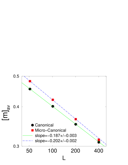
Figure 1: Mean of the bulk magnetization, as defined Eq. (16), for different system sizes, evaluated in the two ensembles. The expected slope from finite size scaling is $\beta/\nu\simeq 0.191$.

The numerical results for the decay of the mean magnetization with system size are shown in Fig. 1. The mean is seen to behave similarly in both ensembles and the system-size decay is consistent with the form expected from finite-size scaling $[m]_{\rm av}\sim L^{-\beta/\nu}$ with $\beta=(3-5^{1/2})/2$ and $\nu=2$, so that $\beta/\nu\simeq 0.191$.

We now look at the distribution of $m$. We use the variable $b=-\ln(m)/L^{1/2}$ since this has good scaling properties. The details of the distributions of $m$, shown in Figs. 2, 3, and 4, are different in the two ensembles; in particular the microcanonical distribution falls off faster at large argument. However, as can be seen in Fig. 4, the behaviour at small values of the argument is the same in both ensembles, which leads to the same asymptotic behaviour for $[m]_{\rm av}$.

Thus, unlike the surface magnetization, the bulk magnetization shows the same critical behaviour in both ensembles. In particular, the results of this section indicate that there is a correlation length which diverges with exponent $\nu=2$ in the microcanonical ensemble. It is not seen in the surface magnetization $m^{s}$, for which the correlation length diverges less strongly with an exponent $\nu=1$, but this must simply indicate that the amplitude of the $\nu=2$ divergence vanishes for $m^{s}$.

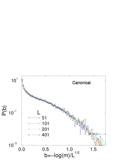
Figure 2: The distribution of the bulk-magnetization for different system sizes for the canonical ensemble.

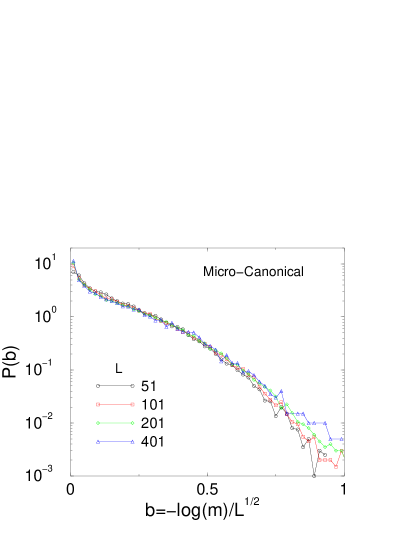
Figure 3: The distribution of the bulk-magnetization for different system sizes for the microcanonical ensemble.

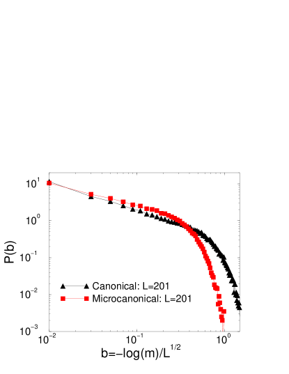
Figure 4: Comparison of the distributions of the bulk-magnetization in the two ensembles for a chain of length $L=201$. On this log-log plot they appear to have the same slope at small values of the argument. However, at large argument, the microcanonical distribution falls off faster.

IV End-to-end correlations and gaps

In this section we investigate numerically the energy gap $\Delta$ and the end-to-end correlation function

$$C_{1L}=\langle 0|\sigma^{z}_{1}\sigma^{z}_{L}|0\rangle$$ (18)

in the canonical and microcanonical ensembles to compare the results of the two ensembles with each other and with analytical resultsFisher and Young (1998) for the canonical ensemble.

We take the following rectangular distribution for the bonds and fields at the critical point

$$\pi(J) = \left\{\begin{array}[]{ll}1&\mbox{for $0<J<1$}\\ 0&\mbox{otherwise}\end{array}\right.$$ (21)

$$\rho(h) = \left\{\begin{array}[]{ll}1&\mbox{for $0<h<1$}\\ 0&\mbox{otherwise.}\end{array}\right.$$ (24)

which gives

$$[\ln h]_{\rm av} = -1,\qquad{\rm var}(\ln h)=1$$

$${[}\ln J]_{\rm av} = -1,\qquad{\rm var}(\ln J)=1.$$ (25)

From this it follows that

$$\ell=L,$$ (26)

where $\ell$ is defined in Eq. (7). We use free boundary conditions without constraining either of the end spins. From Eqs. (3) and (25) the condition for criticality in the microcanonical ensemble is

$$\sum_{i=1}^{L}\ln h_{i}-\sum_{i=1}^{L-1}\ln J_{i}=-1\quad\mbox{(microcan.)}\,.$$ (27)

We initially generate the $h_{i}$ and $J_{i}$ in an unconstrained way, as for the canonical ensemble, but then rescale $h_{i}$ by an appropriate factor so that the above condition is satisfied.

The distributions of $C_{1L}$ and $\Delta$ were studied earlier by Fisher and YoungFisher and Young (1998) and we summarize some of their main results for $L\to\infty$:

$$[C_{1L}]_{\rm av}^{c} \sim \frac{1}{L}$$ (28)

$${[}\Delta]_{\rm av}^{c} \sim L^{1/6}\exp\left[-\frac{3}{2}\left(\frac{\pi^{2}L}{2}\right)^{1/3}\right]$$ (29)

$$\ln(\Delta)-\ln(C_{1L}) = \sum_{i=1}^{L}\ln(h_{l})-\sum_{i=1}^{L-1}\ln(J_{l}).$$ (30)

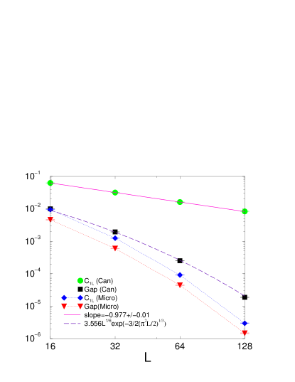
Figure 5: Plot of the mean values of the end-to-end correlation function $C_{1,L}$ and the energy gap $\Delta$ for both the canonical and microcanonical ensembles. In the canonical case, the fits are close to those predicted analytically and given in Eqs. (28) and (29). For microcanonical ensemble, the lines are just guides to the eye.

In Fig. 5 we compare the system size dependence of the average correlation function and the gap in the two ensembles. For the canonical case, the data agree well with the analytic predictions in Eqs. (28) and (29), as was also found in Ref. Fisher and Young, 1998. However, if we fit the data for the gap to Eq. (29) adjusting only the overall amplitude the $\chi^{2}$ is 150 which is very high. Hence there must be systematic corrections to Eq. (29) which are larger for the sizes studied than the, very small, statistical errors.

For the microcanonical ensemble, the data for both $[C_{1L}]_{\rm av}^{mc}$ and $[\Delta]_{\rm av}^{mc}$ in Fig. 5 appear to decay as stretched exponentials, and we will discuss fits to this data below.

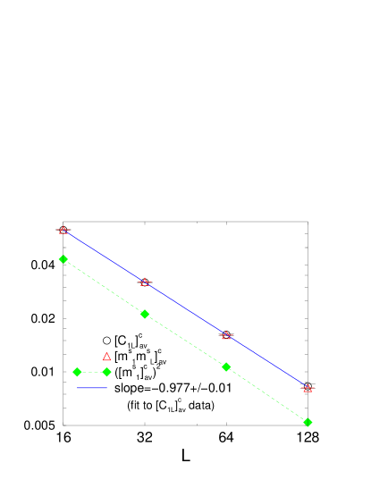
Figure 6: Plot of the mean correlation function $[C_{1,L}]_{\rm av}^{c}$ versus system size compared with $[m_{1}^{s}m_{L}^{s}]_{\rm av}^{c}$ and $([m_{1}^{s}]_{\rm av}^{c})^{2}$, for the canonical ensemble. The $([m_{1}^{s}]_{\rm av}^{c})^{2}$ data falls as $1/L$ as expected from Eq. (14).

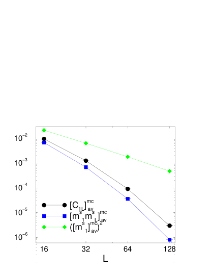
Figure 7: Plot of the mean correlation function $[C_{1,L}]_{\rm av}^{mc}$ versus system size compared with $[m_{1}^{s}m_{L}^{s}]_{\rm av}^{mc}$ and $([m_{1}^{s}]_{\rm av}^{mc})^{2}$, for the microcanonical ensemble. The data for $([m_{1}^{s}]_{\rm av}^{mc})^{2}$ decays as $1/L^{2}$ as expected from Eq. (15).

Interestingly, the value of $[C_{1L}]_{\rm av}$ is found to be close to $[m_{1}^{s}m_{L}^{s}]_{\rm av}$, where $m^{s}_{1}$ ($m^{s}_{L}$) is the surface magnetization at site $1$ ($L$) with the spin at site $L$ ($1$) fixed. This can be seen in Figs. 6 and 7 where we plot both these quantities, as well as $[m_{1}^{s}]_{\rm av}^{2}$, for different system sizes. Especially in the canonical case, $[C_{1L}]_{\rm av}$ and $[m_{1}^{s}m_{L}^{s}]_{\rm av}$ are almost indistinguishable. Note that for the microcanonical, but not the canonical, ensemble $[m_{1}^{s}]_{\rm av}^{2}$ is much greater than $[m_{1}^{s}m_{L}^{s}]_{\rm av}$. The reason for this is that $[m_{1}^{s}]_{\rm av}$ is dominated by a few rare samples where the bonds are bigger than the fields at the free end (and hence, for the microcanonical ensemble, must be less than the fields at the other end because of the constraint). Hence for these samples $m_{L}^{s}$ is smaller than typical in the microcanonical ensemble.

Since $[C_{1L}]_{\rm av}$ and $[m_{1}^{s}m_{L}^{s}]_{\rm av}$ behave similarly we can obtain a better estimate for the decay law in the microcanonical case. This is because $m_{1}^{s}m_{L}^{s}$ can be obtained directly from Eq. (5) and thus be accurately computed numerically for bigger systems. We assume the same form as in the exact result for the gap in the canonical case, Eq. (29), i.e. $aL^{p}\exp(-bL^{\mu})$, and take $\mu=1/3$ the same value as in Eq. (29). The data shown in Fig. 8 is fitted to $aL^{p}\exp(-bL^{1/3})$ by varying $a$ and $b$ for several (fixed) values of $p$. The minimum $\chi^{2}$ of 3.9, which is quite acceptable for three degrees of freedom, is obtained for $p\simeq 0.44$. It we assume that $p=1/6$, as for the canonical case, then $\chi^{2}=1380$ which is extremely high. However, we noted for the canonical case, that there appear to be corrections to the scaling form in Eq. (29). Hence we cannot rule out the possibility that $p=1/6$ also for the microcanonical ensemble.

From Figs. 5 and 7, it seems plausible that $[m_{1}^{s}m_{L}^{s}]_{\rm av}^{\rm mc},~{}[C_{1L}]_{\rm av}^{\rm mc}$ and $[\Delta]_{\rm av}^{\rm mc}$ all vary in the same way in the microcanonical ensemble. If this is so then the data for the gap is consistent with the stretched exponential form $aL^{1/6}\exp(-bL^{1/3})$, for both canonical and microcanonical ensembles, though there are some systematic corrections to this for the range of sizes that can be studied. This is known to be exact for the canonical ensemble, see Eq. (29). It would be interesting to see if the dependence of gap on system size could be determined analytically for the microcanonical ensemble using random walk arguments.

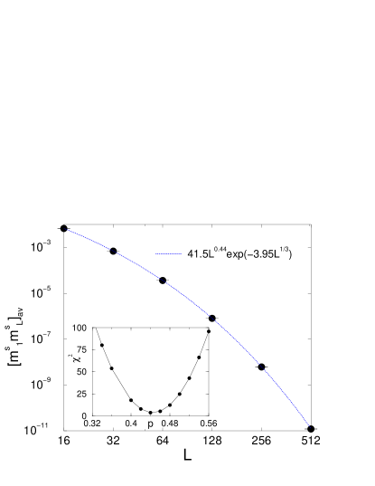
Figure 8: Plot of $[m_{1}^{s}m_{L}^{s}]_{\rm av}^{mc}$ against $L$ for different system sizes, for the microcanonical ensemble. A best fit to the form $aL^{p}e^{-bL^{1/3}}$ with $p=0.44$ ($\chi^{2}=3.9$) is shown. The inset plots $\chi^{2}$ against $p$.

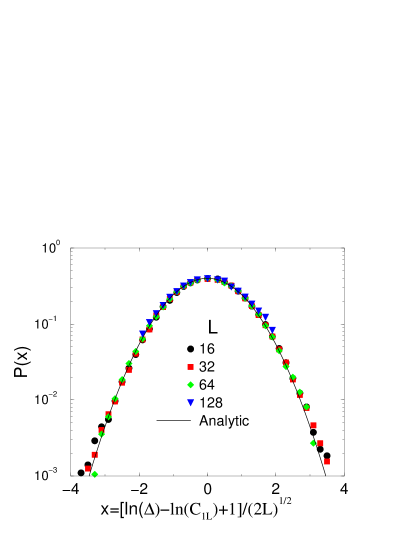
Figure 9: Distribution of $[\ln(\Delta)-\ln(C_{1L})+1]/(2L)^{1/2}$ for the canonical case. The analytic form, deduced from Eq. (30), is a Gaussian with variance unity. This is shown by the solid line.

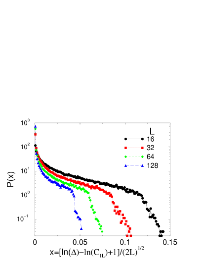
Figure 10: Distribution of $[\ln(\Delta)-\ln(C_{1L})+1]/(2L)^{1/2}$ for the microcanonical case. Equations (27) and (30) predict that $\ln(\Delta)-\ln(C_{1L})+1$ should be identically zero in the thermodynamic limit. The data seems to be tending towards this for large $L$.

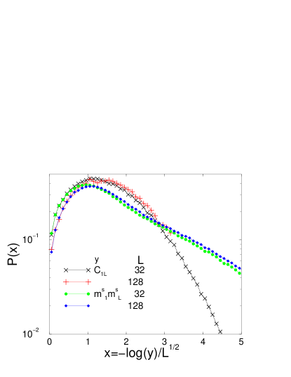
Figure 11: Probability distributions of $C_{1L}$ and $m_{1}^{s}m_{L}^{s}$ for system sizes $L=32$ and $128$ for the canonical ensemble.

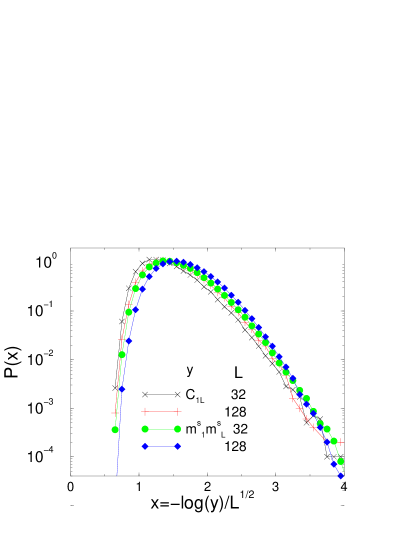
Figure 12: Probability distributions of $C_{1L}$ and $m_{1}^{s}m_{L}^{s}$ for system sizes $L=32$ and $128$ for the microcanonical ensemble.

The distribution of the difference $\ln(\Delta)-\ln(C_{1L})+1$ is plotted in Figs. 9 and 10. In the canonical case, Eqs. (30) and (25) predict a Gaussian distribution with zero mean and standard deviation $\sqrt{2L}$ for large $L$. Fig. 9 shows that this works very well for the full range of sizes studied numerically. Equations (27) and (30) predict that $\ln(\Delta)-\ln(C_{1L})+1$ should be identically zero in the microcanonical ensemble for $L\to\infty$ and hence its distribution should be a delta function at the origin. Indeed the distribution in Fig. 10 is narrow and sharply peaked at zero with a width which deceases as $L$ increases, consistent with these expectations.

Finally we look at the distributions of $C_{1L}$ and $m_{1}^{s}m_{L}^{s}$. The scaling variables are Fisher and Young (1998) $\lambda=-\ln(C_{1L})/L^{1/2}$ and $d=-\ln(m_{1}^{s}m_{L}^{s})/L^{1/2}$ and relevant plots are shown in Figs. 11 and 12 for the canonical and microcanonical ensembles respectively. We see that in the canonical case the overall distributions of $\lambda$ and $d$ are different at large arguments, but they match very accurately at small values of the argument leading to the same behavior for the averages $[C_{1L}]_{\rm av}^{c}$ and $[m_{1}^{s}m_{L}^{s}]_{\rm av}^{c}$ shown in Fig. 6. In the microcanonical case, the overall distributions are quite similar but the agreement at small values of the argument is not as good as in the canonical case. This leads to a greater difference, shown in Fig. 7 between the averages $[C_{1L}]_{\rm av}^{mc}$ and $[m_{1}^{s}m_{L}^{s}]_{\rm av}^{mc}$ than in the canonical case.

To summarize this section, for the canonical ensemble, the end-to-end correlation function $[C_{1L}]_{\rm av}$ falls off at criticality with a power of $L$, as predicted analytically, Eq. (28). However, for the microcanonical ensemble it falls off much faster, as a stretched exponential function of distance. The average gap, $[\Delta]_{\rm av}$ falls off with a stretched exponential form at criticality in both ensembles, with probably the same dependence on $L$.

V Discussion

In this paper we have looked numerically at the finite size dependence of various quantities for the random transverse field Ising chain (RTFIC) at criticality, for both the canonical and microcanonical ensembles of disorder. For quantities that span the system, $m^{s}$ and $C_{1L}$, finite size scaling appears, at first glance, to indicate different correlation length exponents for the two ensembles: $\nu=2$ for canonical and $\nu=1$ for the microcanonical. However, in contrast to Igloi and RiegerIgloi and Rieger (1998), we conclude that the correct interpretation is that the true scaling exponent is the same for the two ensembles, $\nu=2$, but that the amplitude for the leading $\nu=2$ piece is zero, in the microcanonical ensemble, for quantities that span the system and are thus sensitive to the microcanonical constraint. Our reasons for this are two-fold:

1. For the quantity we calculated that does not span the system, the “bulk” magnetization $m$, the same correlation length exponent $\nu=2$ was found for both ensembles, indicating that there is a correlation length in the microcanonical ensemble which diverges with the larger exponent $\nu=2$. Hence, if this is not seen for quantities which span the system, the explanation must be that the amplitude is zero, not that this larger length scale does not exist.

2. The analytical expressions for the distribution of the surface magnetization $m^{s}$, first obtained by FisherFisher , show that the scaling variable is $\bar{\delta}L^{1/2}$ (canonical) and $\delta L^{1/2}$ (microcanonical) demonstrating that the true correlation length exponent is $\nu=2$ in both cases.

Our interpretation of the data implies that the inequalityChayes et al. (1986, 1989) $\nu\geq 2/d$ is satisfied (as an equality) for the RTFIC, in contrast to the conclusion of Pazmandi et al.Pazmandi et al. (1997).

We have also looked at the energy gap between the ground state and first excited state at criticality. For both the canonical and microcanonical ensembles, a stretched exponential decay describes the data. For the canonical case, the exponent $\mu$ (the power of $L$ in the exponential) is exactlyFisher and Young (1998) 1/3, and our numerical data are consistent with $\mu=1/3$ for the microcanonical case too.

The present model, the RTFIC, is integrable and thus relatively simple. In particular, the existence of the simple analytical expression for the surface magnetization $m^{s}$, Eq.(5), is surely related to the integrable nature of the model. Furthermore, the microcanonical constraint $\prod h_{i}=\prod J_{i}$ enters directly in this expression. Thus one can plausibly see how the constraint might affect quantities which span the system and cause amplitudes for these quantities to vanish. However, for non-integrable models, including models in higher dimensions, one would not expect the microcanonical constraint to enter in a direct way even for quantities which span the whole system. Thus it seems unlikely to us that there would be even an apparent difference in the critical behavior of non-integrable models in the two ensembles. We also note that the microcanonical and canonical ensembles of disorder have been investigated for finite-$T$ transitions in random systems by Aharony et al.Aharony et al. (1998) They find no difference asymptotically between the critical behavior and finite-size effects of the canonical and microcanonical ensembles (which they term grand canonical and canonical respectively).

Appendix A

Measurements made in the two ensembles are in fact related to each other by a simple transformation at large $L$. To see this note that

$$\delta=\sum_{i=1}^{L}\xi_{i},$$ (31)

where

$$\xi_{i}=\frac{1}{L}\frac{\ln h_{i}-\ln J_{i}}{{\rm var}(\ln h)+{\rm var}(\ln J)}.$$ (32)

Thus $\delta$ is a sum of $L$ uncorrelated random numbers $\xi_{i},~{}i=1,...L$ with mean

$$[\xi_{i}]_{av}=\bar{\delta}/L$$ (33)

and variance

$$[\xi_{i}^{2}]_{av}-[\xi_{i}]_{av}^{2}=\frac{1}{L^{2}}\frac{1}{{\rm var}(\ln h)+{\rm var}(\ln J)}\,.$$ (34)

Using the central limit theorem and the definition of $\ell$ in Eq. (7) we find that, in a canonical realization with given $\bar{\delta}$ the probability, $P_{\bar{\delta}}(\delta)$, of obtaining the precise value $\delta$ is

$$P_{\bar{\delta}}(\delta)=\left(\frac{\ell}{\pi}\right)^{1/2}e^{-\ell(\delta-\bar{\delta})^{2}},$$ (35)

for $L\to\infty$.

Now let $P^{c}(A,\bar{\delta})$ and $P^{mc}(A,\delta)$ be the probability distributions of some observable $A$ in the canonical and microcanonical ensembles respectively. The two are related by

$$P^{c}(A,\bar{\delta})=\int_{-\infty}^{\infty}P^{mc}(A,\delta)P_{\bar{\delta}}(\delta)\,d\delta.$$ (36)

Correspondingly, expectation values in the two ensembles are related by

$$[A]_{\rm av}^{c}(\bar{\delta})=\int_{-\infty}^{\infty}[A]_{\rm av}^{mc}(\delta)\,P_{\bar{\delta}}(\delta)\,d\delta.$$ (37)

References

- Fisher (1995) D. S. Fisher, Critical behavior of random transverse-field Ising spin chains, Phys. Rev. B. 51, 6411 (1995).
- Fisher and Young (1998) D. S. Fisher and A. P. Young, Critical behavior of random transverse-field Ising spin chains, Phys. Rev. B. 58, 9131 (1998).
- Pazmandi et al. (1997) F. Pazmandi, R. T. Scalettar, and G. T. Zimanyi, Revisiting the theory of finite size scaling in disordered systems: can be less than , Phys. Rev. Lett. 79, 5130 (1997).
- Chayes et al. (1986) J. T. Chayes, L. Chayes, D. S. Fisher, and T. Spencer, Finite-size scaling and correlation lengths for disordered systems, Phys. Rev. Lett. 57, 2999 (1986).
- Chayes et al. (1989) J. T. Chayes, L. Chayes, D. S. Fisher, and T. Spencer, Correlation length bounds for disordered Ising ferromagnets, Commun. Math. Phys. 120, 501 (1989).
- Harris (1974) A. B. Harris, Effect of random defects on the critical behaviour of Ising models, J. Phys. C 7, 1671 (1974).
- Igloi and Rieger (1998) F. Igloi and H. Rieger, Random transverse Ising spin chain and random walks, Phys. Rev. B 57, 11404 (1998).
- Young and Rieger (1996) A. P. Young and H. Rieger, A numerical study of the random transverse-field-Ising spin chain, Phys. Rev. B. 53, 8486 (1996).
- Peschel (1984) I. Peschel, Surface magnetization in inhomogeneous two-dimensional Ising lattices, Phys. Rev. B. 30, 6783 (1984).
- (10) D. S. Fisher, unpublished results.
- Chandrasekhar (1943) S. Chandrasekhar, Stochastic problems in physics and astronomy, Rev. Mod. Phys. 15, 1 (1943).
- Aharony et al. (1998) A. Aharony, A. B. Harris, and S. Wiseman, Critical disordered systems with constraints and the inequality , Phys. Rev. Lett. 81, 252 (1998).