Quantification of Sleep Fragmentation Through the Analysis of Sleep-Stage Transitions

Study Objectives: We introduce new quantitative approaches to study sleep-stage transitions with the goal of addressing the two following questions: (i) Can the new approaches provide more information on the structure of sleep-stage transitions? (ii) How does sleep fragmentation in patients with sleep apnea affect the structure of sleep-stage transitions?
Design: We analyze hypnograms and compare normal subjects and sleep apnea patients using numerous measures, including the percentage of sleep time for each stage, probability distributions of the duration of each stage, the sleep-stage transition matrix, and a measure of the asymmetry of this matrix.
Setting: N/A
Subjects: 197 normal subjects and 50 obstructive sleep apnea patients recruited in the SIESTA project.
Results: We find that the time percentage for wake stage is identical for sleep apnea subjects and for normal subjects, but that the sleep apnea group have a faster decaying distribution of wake duration. Both normal subjects and sleep apnea patients have exponential distributions of duration for all sleep stages and a power law for the wake stage. We also find that there is a loss of preference of transition paths of sleep stages in sleep apnea.
Conclusions: The new approaches proposed here enable us to show that the distribution of sleep and wake duration have different functional forms, indicating fundamental differences in the dynamics between sleep and wake control. The difference remains even in the fragmented sleep of sleep apnea. The fragmentation of sleep in sleep apnea results in a shorter wake duration and interrupts the structure of sleep-stage transitions of sleep apnea subjects, causing the loss of certain particular transition paths.

introduction

Analyses of sleep-stage transitions have long been used as diagnostic tools in clinical applications. Such analyses mostly concentrated on the changes in the time percentage for each sleep stage and in other simple statistics such as the total number of arousals during nocturnal sleep  [1, 2]. There have also been several studies focusing on statistical measures such as transition probabilities  [3, 4, 5, 6, 7], but many other statistical properties of sleep-stage transitions have not been considered in a systematic way.

Sleep-stage transitions are sometimes described as having quasi-cyclic behavior (the sleep cycle)  [2], but on top of the periodic patterns, there are many transitions without apparent periodicity (Fig.  1). Indeed, even if one disregards all sleep-stage transitions and considers only the wake stage during sleep, one still finds intriguing statistical properties and no apparent periodicity  [8]. Furthermore, it has been reported that sleep stages correlate with the dynamics of the autonomic nervous system. For example, the correlations and scaling behavior in heart-rate variability depends on sleep stages  [9, 10]. Because sleep-stage transitions are such complex processes, simple statistical measures may not be sufficient to describe their dynamics and uncover any information contained in the fluctuations. Therefore, we study sleep-stage transitions with methods from modern statistical physics and nonlinear dynamics.

Many advanced statistical analyses have been applied to the study of the electroencephalogram (EEG) during sleep  [11, 12, 13, 14], but an important limitation of these methods is that the EEG records only the activity close to the cortex surface, while it is believed that sleep is regulated by neurons in the hypothalamus [15]. Hence, we hypothesize that to study the dynamics of sleep regulation, one must investigate sleep-stage transitions, which contain more global information, including not only the EEG, but also eye movements and muscle tone.

There are two major limitations in the analysis of sleep-stage transitions: The first is the limited number of data points ($\approx 900$ points per night, where each point represents the sleep stage in a epoch of 30 seconds). The second is the discretization of the data into six sleep stages. These limitations constrict the mathematical tools which can be used in the analysis of sleep-stage transitions, so we focus on the distributions of duration of sleep stages, the transition probability matrices, and the degree of asymmetry of these matrices.

We will also address questions regarding the statistical properties that we find: (i) how do these statistical properties change under the influence of sleep disorders, and (ii) which of these properties are fundamental and do not change under the influence of sleep disorders? To this end, we also study subjects with obstructive sleep apnea, who experience fragmented sleep with a reduced amount of slow-wave sleep and more awakenings (Fig.  1c). The sleep fragmentation is characterized by large number of arousals during nocturnal sleep. When arousal periods are longer than 15 seconds within a 30-second epoch of observation, the epoch is classified as a wake stage. The fragmentation of sleep in obstructive sleep apnea arises from respiratory problems  [16, 17]. Therefore, sleep apnea is a good model for studying the effect of external disturbances on sleep-stage transitions.

In the present study, we propose new quantitative approaches to studying sleep-stage transitions. We show that these approaches enable us to find more information on the structure of sleep-stage transitions and enable us to find how sleep fragmentation of sleep apnea affects the structure of the sleep-stage transitions. Thus, the present approach gives us additional insights into the dynamics of sleep and wakefulness.

Methods

A Subjects and Data acquisition

We analyze a database comprising 197 normal subjects and 50 patients with obstructive sleep apnea collected in eight leading European sleep laboratories under the SIESTA project [18]. For each subject, two consecutive nights were recorded with cardiorespiratory polysomnography. Sleep stages were determined according to the Rechtschaffen and Kales criteria [19]: two channels of electroencephalogram (EEG), two channels of electrooculogram (EOG), and one channel of submental electromyogram (EMG) were recorded. Signals were digitized at a minimum of 100 Hz, and a 12-bit resolution, and are scored visually in epochs of 30 seconds for six stages: wakefulness, rapid-eye-movement (REM) sleep, and non-rapid-eye-movement (NREM) sleep stages 1, 2, 3, and 4. Subjects wend to bed at midnight and were allowed to wake up in the morning at their own well. The average sleep time are xxx for healthy subjects and xxxx for sleep apnea subjects. Wake periods prior to the first sleep stage and after the last sleep stage are excluded from the analyses.

We analyze hypnograms of the second night only. In order to eliminate the effect of age on sleep, we choose 48 of 197 normal subjects and 48 of 50 sleep apnea subjects. The reason for removing two sleep apnea subjects from the group is that these two sleep apnea subjects were much older (74) or younger (29) than the other sleep apnea subjects. We select the normal subjects according to the following procedure: We choose normal subjects from sleep laboratories which also provide sleep apnea subjects. The subjects are chosen to match the ages of 48 sleep apnea subjects. After all age-matched subjects have been chosen, we choose normal subjects randomly from other laboratories, also with similar age, until 48 normal subjects have been selected.

We are thus able to choose normal and sleep apnea subjects with matched ages and maximum possible overlap of source laboratories. The selected normal group has an average age of $50.9$ and a standard deviation of $9.4$, while the selected sleep apnea group has an average age of $51.3$ and a standard deviation of $8.9$. We use the entire database of normal subjects in a test of the reliability of our results.

B Coarse-graining of sleep stages

A major difficulty of studying the statistical properties of sleep-stage transitions is inter-scorer reliability, a topic of great concern in the literature [20, 21, 22, 23, 24]. One study reports that the agreement between sleep-stage scorers are in the range of 30%–90%, depending on the sleep stages and ages of subjects [24]. The least reliable scoring occurs for the NREM stage 1, which has only a 38% agreement on average. All other stages, such as wake, slow-wave sleep, and REM sleep, have an average agreement higher than 70%. To minimize scoring uncertainty, we reduce the six scored stages of sleep into four stages: We keep wake and REM stages unchanged, and group stages 1 and 2 into a single stage (light sleep), and stages 3 and 4 into a single stage (slow-wave sleep). The stages, wake, light sleep, slow-wave sleep, and REM sleep are abbreviated as W, L, S, and R, respectively.

C Percentage of sleep time

We define $F_{m}$ to the percentage of total sleep time for sleep stage $m$. We measure $F_{m}$ for each sleep stage for each subject, and then calculate the mean and standard deviation of $F_{m}$ for normal and sleep apnea groups. We apply Student’s t-test to determine the level of significance of the differences in $F_{m}$ between normal and sleep apnea groups.

D Distributions of duration

$F_{m}$ is a useful tool in diagnostic application, but it cannot capture all the information about the sleep-stage transitions. For example, identical values of $F_{m}$ could result from many short periods or from just a few long periods; two situations with different underlying dynamics. Therefore, we study the distributions of the duration of wake and sleep stages for normal and sleep apnea groups. The distribution of duration of events is a useful measure for studying the underlying dynamics of a system. For example, a peak-like distribution indicates the periodic occurrence of events with fluctuations, such as heart beats intervals [25, 26]. An exponential distribution is usually associated with a random process, such as fluorescent decay [27]. A power-law distribution, which has been observed in many systems, such as earthquakes [28], solar flares [29], and rainfall [30], is associated with self-organized criticality [31, 32] or other complex mechanisms  [33]. Thus, in order to quantitatively study how the brain regulates sleep, we consider the distribution of duration of sleep stages.

We first calculate the duration of the separate wake and sleep stages periods for each subject, then pool the data from all subjects and calculate the group’s cumulative distributions of duration for wake, light sleep, slow-wave sleep, and REM sleep, which we denote as $P_{W}(d)$, $P_{L}(d)$, $P_{S}(d)$, and $P_{R}(d)$, respectively (Appendix A).

E Transition probability matrices

The percentage $F_{m}$ and the distribution of duration $P_{m}(d)$ of each sleep stage provide important information about the sleep stages, but they cannot provide temporal information – i.e., time organization of transitions. For example, $P_{m}(d)$ does not reveal any information about the preferred path of the transitions. Hence, we must study the transition probabilities between different sleep stages.

Several types of transition probabilities for sleep stages have been studied  [5, 6, 7]. Here, we consider a new type of transition probability matrix $T$ with elements $T_{mn}$, defined as $T_{mn}=N_{mn}/N$, where $N_{mn}$ is the number of transitions from stage $n$ to stage $m$ during the entire night and $N$ is the total number of transitions. We calculate the matrix $T$ for each subject and then calculate the means and the standard errors of $T_{mn}$ for normal and sleep apnea groups.

The matrix $T$ is particularly useful for the analysis of the local structure of transitions because it measures the transition probability between two consecutive stages. Since there are a large number of short transitions between different sleep stages even for normal subjects (Fig. 1), the transition matrix may be able to reveal hidden patterns in these short transitions.

F The coefficient of asymmetry of transitions

One of the advantages of studying transition probabilities is that one may be able to extract the information about locally preferred paths in the sleep-stage transitions. One important question is: If there are locally preferred paths, are they affected by the sleep fragmentation of the sleep apnea? To answer this question, we introduce the concept of the symmetry of transitions. When the probability of having a transition from state A to state B is equal to the probability of having one from B to A, transitions between A and B are called “symmetric”. On the contrary, if the probability from A to B is not equal to the probability from B to A, the transition is called “asymmetric”, a pattern indicating a preferred local transition path. In order to quantify the asymmetry in the sleep-stage transitions, we introduce the coefficient of asymmetry $A$ (Appendix B), which can be calculated from the transition matrix. $A=0$ corresponds to a completely symmetric matrix, while $A=1$ corresponds to a completely asymmetric matrix. We calculate $A$ for all subjects and perform Student’s t-test to evaluate the significance of the measured differences in $A$ for normal and sleep-apnea groups.

G Test of the reliability of the results

Since sleep stages are scored visually by different experts in each laboratory, it is important to evaluate how much human bias affects the statistical analyses carried out. We compare our results with the data provided by different laboratories. For example, for the fraction $F_{m}$ of total sleep time for a given sleep stage $m$, we calculated $F_{m}$ for each subject, and compare the distribution of $F_{m}$ of normal subjects from one laboratory to the normal subjects from a different laboratory. We also compare $F_{m}$ of normal subjects from one laboratory to the sleep apnea subjects from the same laboratory and from a different laboratory. We perform the same procedure on all other statistical measures calculated in this study. We calculate the $p$ value for Student’s t-test [34] and find the differences between normal and apnea subjects are much more significant ($p<0.05$) than the differences between normal subjects from different laboratories ($p>0.05$).

Results

We first show results for the time percentage $F_{m}$ for each sleep stage for both normal and sleep apnea groups (Fig. 2). We find significant differences between the two groups for stage 1 ($p<0.001$) and also for stage 4 ($p<0.05$). However, there are no significant differences between normal and sleep apnea groups for the wake stage, sleep stage 2, and REM sleep.

In Fig. 3 we show distributions of duration for wake, $P_{W}(d)$, light sleep, $P_{L}(d)$, slow-wave sleep, $P_{S}(d)$, and REM sleep, $P_{R}(d)$, for normal and sleep apnea groups. $P_{W}(d)$ shows a power-law decay $P_{W}(d)\propto d^{-\alpha}$ for both normal and sleep apnea groups, while $P_{L}(d)$, $P_{S}(d)$, and $P_{R}(d)$ all show exponential decays, $P(d)\propto e^{-d/\tau}$.

We compare $P_{W}(d)$, $P_{L}(d)$, $P_{S}(d)$, and $P_{R}(d)$ for normal and sleep apnea subjects and find that (i) $P_{W}(d)$ for sleep apnea group has a larger exponent $\alpha=1.28\pm 0.03$ than the normal group, $\alpha=1.11\pm 0.05$, and (ii) $P_{L}(d)$, $P_{S}(d)$, and $P_{R}(d)$ for the sleep apnea group show a steeper decay in the region $d<5$ min, but their decay time scale $\tau$ in the longer time region are similar to those of the normal group.

We show the transition probability matrices $T$ for the normal and sleep apnea groups in Tables 1a& b. Not surprisingly, for both normal and sleep apnea subjects, we find some transitions are virtually prohibited: (i) there are no $R\rightarrow S$ transitions and only few $S\rightarrow R$ transitions, and (ii) there is no $W\rightarrow S$ transition.

For both the normal and sleep apnea groups, the matrices are asymmetric, but this asymmetry decreases for the sleep apnea group. To quantify the degree of asymmetry for normal and sleep apnea groups, we calculate the coefficient of asymmetry $A$ for the data from each subject and plot distributions of $A$ for normal and sleep apnea groups (Fig. 4). The normal group has a mean $A$ of $0.058\pm 0.004$, while the sleep apnea group has a mean $A$ of $0.034\pm 0.003$.

We perform Student’s t-test to calculate the level of significance of the difference in $A$ between normal and sleep apnea groups, resulting in a $p$ value smaller than $1\times 10^{-5}$.

We also test to see if $A$ changes for elder subjects, who are known to show more arousals during nocturnal sleep  [1]. We choose two groups from our database of 197 normal subjects: young (47 subjects, age: 20–35 years), and old (52 subjects age: 60–75 years). We find that the number of sleep-stage transitions in the older group has a mean of $106\pm 3$, which is significantly larger than the mean of $84\pm 2$ for the young group.

We compare distributions of $A$ between these two groups. The young group has an average $A$ of $0.061\pm 0.005$, while the old group has an average $A$ of $0.051\pm 0.004$. Applying Student’s t-test, we find $p=0.6$.

A comparison of $F_{m}$, $P_{m}(d)$ and $A$ of normal group with sleep apnea group is shown in Table 2.

Discussion

We have proposed new approaches to the characterization of the dynamics of sleep-stage transitions, and found several intriguing properties:

1. We find that for normal subjects, the duration of each sleep stage is characterized by an exponential distribution with specific time scale, and the duration of wake stage is characterized by a power-low distribution suggesting a scale-free dynamics. This finding suggests a fundamental difference between the dynamics of sleep and wakefulness control. It implies that sleep and wakefulness are not just two parts of a sleep-wake control, but that there exist entirely different mechanisms for their regulation in the brain, which supports recent studies in the neuronal level of sleep mechanisms (see, e.g., Ref. [15]).

   Ref. [8] reported that, for normal subjects, the duration of wake periods follows a power-law distribution, $P_{W}(d)\propto d^{-\alpha}$, while the duration of sleep periods follows an exponential distribution, $P(d)\propto e^{-d/\tau}$. As shown in Fig. 3, when we decompose sleep into three stages: light, slow-wave and REM sleeps, all these sleep stages still follow exponential distributions. It is surprising that REM sleep, which can be regarded as somehow similar to wake from a brain activity aspect, clearly follows an exponential distribution of duration as the rest of the sleep stages, which is different from the power-law distribution of duration of the wake stage.

   The same forms of the distributions are observed for sleep apnea patients for all sleep stages (exponential) and for the wake stage (power law). This finding suggests robust mechanisms of sleep and wakefulness controls which do not change with sleep fragmentation in sleep apnea.

2. Our finding that the time percentage $F_{W}$ for the wake stage of the sleep apnea group is not significantly different from that of the normal group appears to contradict the “common” expectation that sleep apnea subjects have more arousals. However, the difference in the wake stage between normal and sleep apnea subjects is clearly observed in the distributions of wake duration $P_{W}(d)$. The difference in the values of the power-law exponent $\alpha$ characterizing $P_{W}(d)$ (Fig. 3) indicates that wake periods for sleep apnea subjects have shorter duration. Since $F_{W}$ is identical, sleep apnea subjects must have a larger number of wake periods. This is a clear indication of the sleep fragmentation one expects for sleep apnea.

   Although the functional form of $P_{L}(d)$, $P_{S}(d)$ and $P_{R}(d)$ is identical for normal and sleep apnea groups, the characteristic time scales are different, except for REM sleep. We find that the most significant change occurs for short duration (Fig. 3b&d). The increasing of slopes in the short duration $d<5$ min, indicates that sleep apnea subjects have many more short stages than normal subjects do, and thus a more fragmented sleep.

   Note that the power-law exponent $\alpha=1.1$ for $P_{W}(d)$ for normal subjects (Fig. 3b). This value is different from what we reported ($\alpha=1.3$) previously  [8]. The reason is that in Ref. [8] our results was based on the database of 20 young subjects with average age of $35.2$, which is different from the average age of $50.9$ of the 48 normal subjects we used in this study. With the choice of young normal subjects from the database we used in the present study, we recover $\alpha=1.3$, which in agreement with the value reported in Ref. [8].

3. From the transition matrix $T$ we find that the transition probabilities between several pairs of stages change with sleep apnea. These changes can be characterized by the coefficient of asymmetry. Both normal and sleep apnea groups have asymmetric transition matrix $T$, but the sleep apnea group exhibits an increase of symmetry. The implication of an asymmetric transition matrix is that the transition process has preferred transition paths. Comparing $T_{RL}$ and $T_{LR}$, we find that there are more transitions from light sleep to REM sleep than from REM sleep to light sleep. We also find, by comparing $T_{WR}$ and $T_{RW}$, that there are more transitions from REM to wake then from wake to REM. These findings indicate that when a $R\rightarrow W$ transition occurs, the sleep control system “prefers” to make a transition to light sleep instead of back to REM (Fig. 5a). The explanation is supported by the values of $T_{LW}$ and $T_{WL}$: there are more $W\rightarrow L$ transitions than $L\rightarrow W$ transitions.

   We find that the matrices exhibit increased symmetry for the sleep apnea group (Fig. 4). This indicates that the sleep-stage transitions of sleep apnea subjects have less local structure. From the distributions of wake duration, we learn that sleep apnea subjects have a larger number of transitions but shorter duration. The increased wake periods, according to transition matrices, increase the symmetry of the matrix by distributing with less preference throughout the night (Fig. 5b).

4. A question one may ask is if the increase of the symmetry is a necessary result of the increase of the number of wake periods? As described in the results section, we calculate $A$ for elderly subjects which have significantly larger number of wake periods during sleep. It is very interesting that although elderly subjects experience a larger number of wake periods, the coefficient of asymmetry does not change significantly ($p=0.06$). This might indicate that the preferred transition path observed in normal subjects is fundamental, and is not significantly affected by age: The increased wake periods do not significantly change the preference of sleep-stage transition in elder subjects, while the increased wake periods in sleep apnea subjects do.

All of our analyses are based on group distributions. However, both normal and sleep apnea groups have broad distributions for many statistical measures. It is not known whether the changes in group distributions are representative of changes in the individual behavior. It is also not known if each individual in the normal group (or in the sleep apnea group) follows the same statistics. To answer the questions, data of at least ten nights from each subject are needed. One can then compare the distribution of statistical measures from data on one subject to the data on another subject.

Furthermore, all the analyses are based on whole-night records. However, sleep is not a homogeneous process. The statistical properties may vary throughout the night  [35, 2, 8]. Hence, it is important to study the changes in $P_{m}(d)$, $T$ and $A$ in the course of the night.

Our findings of the stability of underlying dynamics of sleep-stage transitions between normal and sleep apnea subjects are intriguing. It is important to test if the dynamics changes under pharmacological influences such as sleep-inducing drugs or caffeine, or under different psycho-physiological or pathological conditions such as stress or depression.

Appendix

A. Cumulative distribution of duration

Let $p_{m}(d)$ be the probability density function (i.e. the probability distribution) for the duration $d$ of a given stage $m$ for the group. We study the cumulative distribution $P_{m}(d)$, which is defined as:

$$P_{m}(d)\equiv\int_{d}^{\infty}p_{m}(r)dr\,.$$

Therefore, $P_{m}(d)$ is the probability of having a period of stage $m$ with a duration longer than $d$. The reasons to consider $P_{m}(d)$ instead of $p_{s}(d)$ are: (i) $P_{m}(d)$ gives curves smoother than $p_{m}(d)$ does, making analyses easier. (ii) $P_{m}(d)$ does not lose any information carried in $p_{m}(d)$, and (iii) $P_{m}(d)$ preserve shapes for power-law and for exponential functional forms.

B. The coefficient of asymmetry

The coefficient of symmetry of $A$ is defined as

$$A=\frac{1}{3}\biggl{[}\bigl{(}\frac{T_{WR}-T_{RW}}{T_{WR}+T_{RW}}\bigr{)}^{2}+\bigl{(}\frac{T_{LW}-T_{WL}}{T_{LW}+T_{WL}}\bigr{)}^{2}+\bigl{(}\frac{T_{LR}-T_{RL}}{T_{LR}+T_{RL}}\bigr{)}^{2}\biggr{]}^{1/2},$$

where the $T_{mn}$ are elements in the transition probability matrix defined in the Methods section. For a completely symmetric matrix in which $T_{mn}=T_{mn}$, $A=0$, while for a completely asymmetric matrix in which one of $T_{mn}$ and $T_{nm}$ is equal to $0$, $A=1$.

FIGURE 1

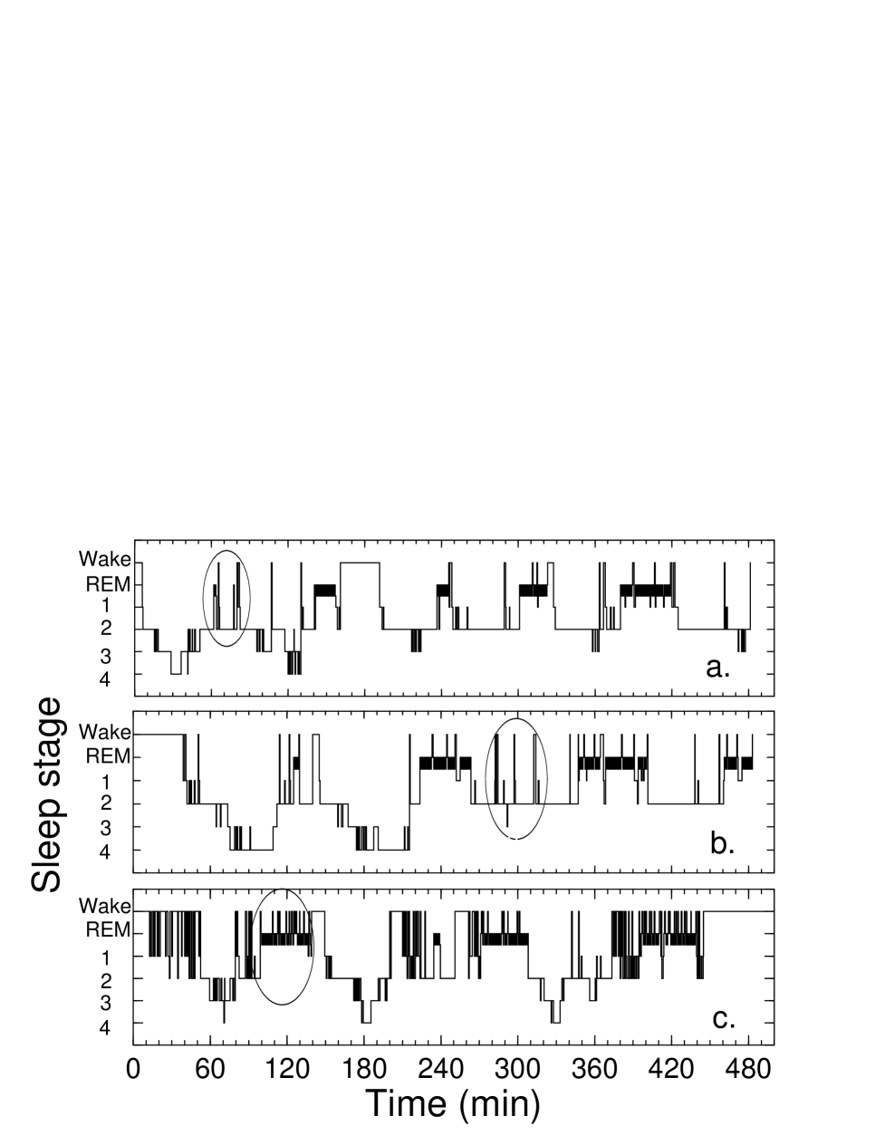
FIG. 1.: Three typical hypnograms for normal subjects (a) and (b), and for a sleep apnea subject (c). There are large number of short sleep-stage transitions as shown in ovals throughout the nights for both normal and sleep apnea subjects. The overall patterns of hypnograms between different normal subjects are also very different. The sleep apnea subject experience fragmented sleep, and shows a much larger number of short transitions than normal subjects do.

FIGURE 2

FIG. 2.: Fraction $F_{m}$ of total sleep time for a given stage $m$. Here we show the average values based on a database of 48 normal subjects and 48 sleep apnea subjects with matched ages. The error bars give uncertainties of the average values. Student’s t-test is performed to measure the significance of the difference between normal and the sleep apnea groups. One asterisk indicates $p<0.05$, and two asterisks indicate $p<0.01$. Sleep stages 1 and 4 display significant differences between normal and sleep apnea subjects, while wake, stage 2, 3 and REM do not display significant differences. Further on we consider only four stages: wake (W), light sleep (L), slow-wave sleep (S), and REM sleep (REM), therefore we show the percentage of total sleep time for these four stages in the inset.

FIGURE 3

Normal

Sleep apnea

FIG. 3.: Cumulative distribution of duration for each sleep stage showing different features for wake stage and sleep stages but similar features for normal and sleep apnea subjects. (a) Semi-logarithmic plot and (b) double-logarithmic plot show curves for the normal group. (c) Semi-logarithmic plot and (d) double-logarithmic plot show curves for the sleep apnea group. For both normal and sleep apnea groups, the distributions for wake follow power-law decays, while the distributions for all sleep stages follow exponential decays. Comparing to the normal group, the sleep apnea group shows larger power-law exponent $\alpha$ for the distribution of wake duration, larger characteristic time scale $\tau$ for the distribution of duration of light sleep, but similar characteristic time scale for the distributions of duration of slow-wave and REM sleep. In order to compare curves of light, slow-wave and REM sleep in the small time region ($d<5$ min) between normal and sleep apnea subjects, power-law functions are fit to the curves of light and slow-wave sleep for $d<5$ min (c & d). Note that the fitting is only for the purpose of comparison. The lack of data points in the region of $d<5$ min makes it difficult to determine the functional form of the distribution for sleep stages in this small-time region. Note that for distributions of all sleep stages, the sleep apnea group shows a steeper decay in the small time region ($d<5$ min).

FIGURE 4

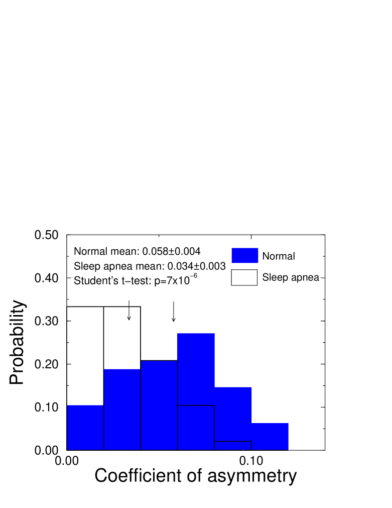
FIG. 4.: Distribution of the coefficient of symmetry (defined in the text) for normal and sleep apnea groups. Arrows indicate means of distributions of normal and sleep apnea groups. The result of Student’s t-test indicates that the observed averages of these two groups are significantly different, suggesting that the sleep apnea group has a significant decrease of the asymmetry as the result of the sleep fragmentation.

FIGURE 5

Normal

Sleep Apnea

FIG. 5.: Illustration of asymmetric sleep-stage transitions. Since wake periods are much shorter than the light, slow-wave and REM sleep periods on average, we assume that the basic structure of sleep-stage transitions are dominated by light sleep, slow-wave sleep and REM sleep. (a) Wake periods can be viewed as spikes distributed throughout the night in light and REM sleep. Because $T_{WR}>T_{RW}$ for normal subjects (cf. Table 2, where $T_{WR}/T_{RW}\approx 5.6$), there is a preference for transitions from REM to wake and then to light sleep, instead of back to REM. (b) For sleep apnea subjects, there is increasing symmetry in transitions (cf. $T_{WR}/T_{RW}\approx 2.6$). Because sleep apnea subjects have more transitions on average, the increased wake periods may distribute in light and REM sleep with less preference throughout the night.

Table 1

a) Transition probability matrix $T_{mn}$ (defined in the text) for normal subjects, where $m$ corresponds to row and $n$ corresponds to column. The numbers in the matrix are means of the group distributions and standard errors of means.
The average number of transitions per night $=96.0\pm 3.2$.

$$\begin{matrix}&&W&&R&&L&&S\\ &&&&&&&&\\ W&&-&&0.050\pm 0.005&&0.182\pm 0.009&&0.016\pm 0.002\\ R&&0.009\pm 0.002&&-&&0.116\pm 0.007&&0.004\pm 0.001&\\ L&&0.237\pm 0.010&&0.073\pm 0.006&&-&&0.139\pm 0.010\\ S&&0.001\pm 0.001&&0.000\pm 0.000&&0.155\pm 0.010&&-\\ \end{matrix}$$

b) Same as above for sleep apnea.
The average number of transitions per night $=123.0\pm 6.2$.

$$\begin{matrix}&&W&&R&&L&&S\\ &&&&&&&&\\ W&&-&&0.042\pm 0.004&&0.217\pm 0.014&&0.008\pm 0.002\\ R&&0.016\pm 0.004&&-&&0.126\pm 0.012&&0.001\pm 0.001\\ L&&0.250\pm 0.014&&0.099\pm 0.011&&-&&0.105\pm 0.010\\ S&&0.001\pm 0.001&&0.000\pm 0.000&&0.114\pm 0.010&&-\\ \end{matrix}$$

Table 2

Table 2. Summary of results of our analysis for (i) the mean time percentage, (ii) the distribution of duration of sleep stages and (iii) the mean degree of asymmetry of the transition probability matrix.

	$\bar{F}_{m}$ (%)					$P_{m}(d)$
Subjects	W	L*	S*	R		W*	L*	S	R	$\bar{A}$*
Normal	10.6	57.3	12.2	17.8		$d^{-1.1}$	$e^{-d/9.9}$	$e^{-d/10.4}$	$e^{-d/9.3}$	0.58
Sleep Apnea	10.1	61.8	8.9	17.0		$d^{-1.3}$	$e^{-d/10.9}$	$e^{-d/10.9}$	$e^{-d/9.2}$	0.34

Symbols: $\bar{F}_{m}$, mean time percentage for stage $m$. $P_{m}(d)$, distribution of duration $d$ of stage $m$. $\bar{A}$, mean degree of asymmetry. Stage $m$ can be wake ($W$), light sleep ($L$), slow-wave sleep ($S$) or REM ($R$).

An asterisk denotes significant difference between normal and sleep apnea groups.

REFERENCES

- [1] Chokroverty S. An overview of sleep. In: Chokroverty S ed. Sleep Disorders Medicine. Boston: Butterworth Heinemann, 1999: 7–20.
- [2] Carskadon MA, Dement WC. Normal Human Sleep: An Overview. In: Kryger MH, Roth T, Dement WC eds. Principles and Practice of Sleep Medicine. Philadelphia: WB Saunders Co, 2000: 15–25.
- [3] Williams R, Agnew H, Webb W. Sleep patterns in young adults: an EEG study. Electroen Clin Neuro 1964; 17: 376-381.
- [4] Brezinova V. The number and duration of the episodes of the various EEG stages of sleep in young and older people. Electroen Clin Neuro 1975; 39: 273-278.
- [5] Kemp B, Kamphuisen HAC. Simulation of human hypnograms using a Markov chain model. Sleep 1986; 9: 405-414.
- [6] Yassouridis A, Steiger A, Klinger A, Fahrmeir L. Modeling and exploring human sleep with event history analysis. J Sleep Res 1999; 8: 25-36.
- [7] Karlsson MO, Schoemaker RC, Kemp B, Cohen AF, van Gerven JMA, Tuk B, Peck CC, Danhof M. A pharmacodynamic Markov mixed-effects model for the effect of temazepam on sleep. Clin Pharmacol Ther 2000; 68: 175-188.
- [8] Lo CC, Amaral LAN, Havlin S, Ivanov PCh, Penzel T, Peter J-H, Stanley HE. Dynamics of sleep-wake transitions during sleep. Europhys Lett 2002; 57: 625-631.
- [9] Ivanov PCh, Bunde A, Amaral LAN, Havlin S, Fritsch-Yelle J, Baevshk RM, Stanley HE, Goldberger AL. Sleep-wake differences in scaling behavior of the human heartbeat: Analysis of terrestrial and long-term space flight data. Europhys Lett 1999; 48: 594-600.
- [10] Bunde A, Havlin S, Kantelhardt JW, Penzel T, Peter JH, Voigt K. Correlated and uncorrelated regions in heart-rate fluctuations during sleep Phys Rev Lett 2000; 85: 3736-3739.
- [11] Fell J, Röschke J, Schaffner C. Surrogate data analysis of sleep electroencephalograms reveals evidence for nonlinearity. BIOLOGICAL CYBERNETICS 1996; 75: 85-92.
- [12] Pradhan N, Sadasivan PK. The nature of dominant Lyapunov exponent and attractor dimension curves of EEG in sleep. COMPUTERS IN BIOLOGY AND MEDICINE 1996; 26: 419-428.
- [13] Pereda E, Gamundi A, Rial R, Gonzalez J. Non-linear behaviour of human EEG: fractal exponent versus correlation dimension in awake and sleep stages. Neurosci Lett 1998; 250: 91-94.
- [14] Fell J, Kaplan A, Darkhovsky B, Röschke J. EEG analysis with nonlinear deterministic and stochastic methods: a combined strategy. Acta Neurobiol Exp 2000; 60: 87-108.
- [15] Saper CB, Chou TC, Scammell TE. The sleep switch: hypothalamic control of sleep and wakefulness. Trends Neurosci 2002; 24: 726-731.
- [16] Strollo PJ, Rogers RM. Current concepts: Obstructive sleep apnea. New Engl J Med 1996; 334: 99-104.
- [17] Robinson A, Guilleminault C. Obstructive sleep apnea syndrome. In: Chokroverty S ed. Sleep Disorders Medicine. Boston: Butterworth Heinemann, 1999: 331–354.
- [18] Klösch G, Kemp B, Penzel T, Schlögl A, Rappelsberger P, Trenker E, Gruber G, Zeitlhofer J, Saletu B, Herrmann WM, Himanen SL, Kunz D, Barbanoj MJ, Röschke J, Värri A, Dorffner G. The SIESTA project polygraphic and clinical database. IEEE Eng Med Biol 2001; 20: 51-57.
- [19] Rechtschaffen A, Kales A. Manual of Standardized Terminology, Techniques, and Scoring System for Sleep Stages of Human Subjects. Los Angeles: California BIS/BRI, University of California; 1968.
- [20] Kelley JT, Reilly EL, Overall JE, Reed K. Reliability of rapid clinical staging of all night EEG. Clin Electroencephalogr 1985; 16: 16-20.
- [21] Kubicki S, Holler L, Berg I, Pastelak-Price C, Dorow R. Sleep EEG evaluation: a comparison of results obtained by visual scoring and automatic analysis with the Oxford sleep stager. Sleep 1989; 12: 140-149.
- [22] Whitney CW, Gottlieb DJ, Redline S, Norman RG, Dodge RR. Reliability of scoring respiratory disturbance indices and sleep staging. Sleep 1998; 21: 749-757.
- [23] Norman RG, Pal I, Stewart C, Walsleben JA, Rapoport DM. Interobserver agreement among sleep scorers from different centers in a large dataset. Sleep 2000; 23: 901-908.
- [24] Kunz D, Danker-Hopfe H, Gruber G, Klösch G, Lorenzo JL, Himanen SL, Kemp B, Penzel T, Röschke J, Dorffner G. Interrater reliability between eight European sleep-labs in healthy subjects of all age groups. J Sleep Res 2000; 9: Supp 1: 106.
- [25] Peng CK, Mietus J, Hausdorff JM, Havlin S, Stanley HE, Goldberger AL. Long-range anti-correlations and Gon-Gaussian behavior of the heartbeat. Phys Rev Lett 1993; 70: 1343-1346.
- [26] Ivanov PCh, Rosenblum MG, Peng CK, Mietus J, Havlin S, Stanley HE, Goldberger AL. Scaling behaviour of heartbeat intervals obtained by wavelet-based time-series analysis. Nature 1996; 383: 323-327.
- [27] Campbell ID, Raymond AD. Biological spectroscopy. Menlo Park: Benjamin/Cummings Pub Co, 1984: 91–125.
- [28] Bak P, Christensen K, Danon L, Scanlon T. Unified scaling law for earthquakes. Phys Rev Lett 2002; 88: art. no. 178501.
- [29] Boffetta G, Carbone V, Giuliani P, Veltri P, Vulpiani A. Power Laws in Solar Flares: Self-Organized Criticality or Turbulence? Phys Rev Lett 1999; 82: 4662-4665.
- [30] Peters O, Hertlein C, Christensen K. A Complexity View of Rainfall. Phys Rev Lett 2002; 88: art. no. 18701.
- [31] Bak P. How nature works : the science of self-organized criticality. New York: Copernicus, 1996.
- [32] Sánchez A, Newman DE, Carreras BA. Waiting-Time Statistics of Self-Organized-Criticality Systems. Phys Rev Lett 2002; 88: 68320.
- [33] Sornette D. Critical phenomena in natural sciences: chaos, fractals, selforganization, and disorder : concepts and tools. Berlin: Springer, 2000: 285-320
- [34] Press WH, Teukolsky SA, Vetterling WT, Flannery BP. Numerical recipes in C. Cambridge: Cambridge University Press; 1994. 616-617
- [35] Born J, Hansen K, Marshall L, Molle M, Fehm HL. Timing the end of nocturnal sleep. Nature 1999; 397: 39-30.