Magnetic phenomena in 5d transition metal nanowires

Abstract

We have carried out fully relativistic full-potential, spin-polarized, all-electron density-functional calculations for straight, monatomic nanowires of the $5d$ transition and noble metals Os, Ir, Pt and Au. We find that, of these metal nanowires, Os and Pt have mean-field magnetic moments for values of the bond length at equilibrium. In the case of Au and Ir, the wires need to be slightly stretched in order to spin polarize. An analysis of the band structures of the wires indicate that the superparamagnetic state that our calculations suggest will affect the conductance through the wires — though not by a large amount — at least in the absence of magnetic domain walls. It should thus lead to a characteristic temperature- and field dependent conductance, and may also cause a significant spin polarization of the transmitted current.

I introduction

There is presently a strong interest in the physics of metal nanowires of atomic dimensions. A freely hanging metallic nanowire is formed when two pieces of material, initially at contact, are pulled away from each other over atomic distances. In the process a connective bridge or neck elongates and narrows. Experimentally, segments of such nanowires have been formed between tips, in particular of Au,kondo2000_helical ; rodrigues2000 but very recently also in break junctions of Pt and Ir.smit2001 . The one-dimensional character of nanowires cause several new physical phenomena to appear, like quantized conductancewees1988 and helical geometries.gulseren1998 ; kondo2000_helical ; tosatti2001_tension With respect to the bulk metal, the freely hanging nanowires are of course unstable and therefore transient objects, which undergo thinning and eventual breaking. Nevertheless, the kinetics leading to that thinning process slows down when reaching special “magic” geometries, where long lifetimes of several seconds have been recorded. The occurrence of magic geometries has been proposed to correspond to local minima of the nanowire effective string tension.tosatti2001_tension Some of these wires are only a few atomic layers thick, but can extend in length up to 15 nm, which corresponds to roughly 50 gold-atom diameters.kondo2000_helical Ultimately thin wires, consisting of only a single atomic strand, so-called monowires — necessarily much shorter than the above mentioned thicker wires — have also been observed.smit2001 ; ohnishi1998 ; yanson1998 Besides these transient objects, another type of nanowires, which are stable, also exist. Structurally stable nanowires can be grown on stepped surfaces, like for example the recently observed Co monatomic chains on Pt substrate,gambardella2002 or inside tubular structures, like the Ag nanowires of micrometer lengths grown inside self-assembled calix[4]hydroquinine nanotubes.heehong2001

An interesting question is of course if, when and how magnetism may appear in nanowires and how — if that is the case — this affects the other properties. Those metals, which are magnetic already in bulk, can be expected to be magnetic also as nanowires, Hund’s rule being reinforced by lower coordination. But may also normally non-magnetic metals magnetize in nanowires form? It has been suggested that even a jellium confined in a thin cylinder may in principle magnetize for certain radii of the cylinder.zabala1998 However, the moment formation is confined to very special radii or electron densities, and the associated energy gain is very small. That is of course so because exchange interactions, as described by Hund’s first rule, are not particularly strong in an $sp$ band metal (e.g., Na or Al), a typical system that might be thought of as a jellium. The situation is radically different for transition metals of the $4d$ and $5d$ series. Because of the partly occupied $d$ orbitals, their ability to magnetize is much stronger and of a fundamentally different nature compared to the jellium. In bulk, the resulting large exchange interactions of these metals are overwhelmed by the large electron kinetic energies, resulting in very large bandwidths and a nonmagnetic ground state.

In the present work, we concentrate on monatomic wires made up of the $5d$ elements Os, Ir, Pt and Au, investigating the possibility of ferromagnetismnote1 in these nanowires. Of these metals, Os and Ir exhibit monolayer magnetism on Au or Ag substrates.blugel1992 ; redinger1995 Os, Ir, and Pt might conceivably develop Hund’s rule magnetism in free-hanging nanowire form, due to their partly empty $d$ shell. Au, on the other hand, is basically an $sp$ metals but with some $d$ orbitals quite close to the Fermi level, making it a borderline case. If strong Hund’s rule magnetism develops in these wires, the number of conductance channels would be greatly influenced, and the results could show up in the form of, e.g., strong and unusual joint magnetic field and temperature dependence in the ballistic conductance.

Of course, thermal fluctuations in nanowires are expected to be very large, which would destroy long range magnetic order in the absence of an external magnetic field. Depending on temperature and on external field, there will nevertheless be two different fluctuation regimes: a slow one and a fast one.

Slow fluctuations such as those attainable at low temperatures and/or in presence of a sufficiently large external field take a nanomagnet to a superparamagnetic state, where magnetization fluctuates between equivalent magnetic valleys, separated by, e.g., anisotropy-induced energy barriers. If the barriers are sufficiently large the nanosystem spends most of the time within a single magnetic valley, and will for many practical purposes behave as magnetic. We may under these circumstances be allowed to neglect fluctuations altogether, and to approximate some properties of the superparamagnetic nanosystem with those of a statically magnetized one. Experimentally, evidence of one-dimensional superparamagnetism with fluctuations sufficiently slow on the time scale of the probe was recently reported for Co atomic chains deposited at Pt surface steps.gambardella2002

At the opposite extreme — a situation reached for example at high temperatures, and in zero external field — the energy barriers are so readily overcome that the magnetic state will be totally washed away by fast fluctuations, leading to a conventional paramagnetic state. A complete description of this high entropy state is beyond scope here, and we have chosen, as is usually done, to approximate it with the conventional $T=0$ nonmagnetic, singlet solution of the Kohn-Sham electronic structure equations.

In this paper we will only deal with straight undimerized wires. This might appear oversimplified, since, for instance, it has been calculated that infinite gold wires have a local energy minimum for a zigzag structure.sanchezportal1999 Similar structures are also possible for the other metals studied here. Our rationale for this simplification of the wire geometry is that wires extended between two tips are inevitably subject to stretching. The simple thermodynamics causing the wire-tip atom flow of atoms and driving the thinningtorres1999 implies a finite string tension.tosatti2001_tension Thus, even if a free-ended wire favored a zigzag structure, this effect will be washed out in the ultimate wire hanging between tips just before breaking of the contact. Moreover possible dimerization of the wires, an issue whose possible relevance is restricted to gold, will not be considered here.

II method

In the present density-functional-baseddft electronic-structure calculations we used the all-electron full-potential linear muffin-tin orbital method (FP-LMTO).wills This method assumes no shape approximation of the potential or wave functions. The calculations were performed using the generalized gradient approximation (GGA).gga As a test, some calculations were also performed using the local density approximation (LDA),lda , giving results very similar to the GGA ones. Further, some calculations were double-checked using the WIEN code,wien97 again with very similar results. We chose an all-electron approach in order to rid our calculations of possible sources of doubt that may arise when using pseudopotentials in the presence of magnetism and in non-standard configurations.

The calculations were performed with inherently three-dimensional codes, and thus the system simulated was an infinite two-dimensional array of infinitely long, straight wires. A one-dimensional Brillouin zone was used, i.e the k-points form a single line, stretching along the $z$-axis of the wire. The Bravais lattice in the $xy$-plane was chosen hexagonal. Furthermore, we used non-overlapping muffin-tin spheres with a constant radius in the calculations of the equilibrium bond lengths $d$. The magnetic moments, bands structures, conductance-channel curves and band widths were calculated using muffin-tin spheres scaling with the bond length. Convergence of the magnetic moment was ensured with respect to k-point mesh density, Fourier mesh density, tail energies, and wire-wire vacuum distance.

We performed both scalar relativistic (SR) calculations, and calculations including the spin-orbit coupling as well as the scalar-relativistic terms. The latter will be referred to as “fully relativistic” (FR) calculations in the following, although we are not strictly solving the full Dirac equation, or making use of current density functional theory. In the FR calculations, the spin axis was chosen to be aligned along the wire direction.

III results and discussion

Table 1: Calculated monowire and bulk equilibrium bond length $d$. Also shown are the calculated magnetic moments per atom, with and without spin-orbit coupling, at the monowire equilibrium bond length. The right-most column displays the experimental ground-state configuration for the free atoms.

	wire	wire	bulk	bulk	moment	moment	free
	$d$ (Å)	$d$ (Å)	$d$ (Å)	$d$ (Å)	($\mu_{B}$)	($\mu_{B}$)	atom
metal	SR	FR	FR	exp.	SR	FR	moment
Os	2.31	2.30	2.76	2.73	1.3	0.3	4 (${}^{5}D_{4}$)
Ir	2.31	2.34	2.75	2.71	0.8	-	3 (${}^{4}F_{9/2}$)
Pt	2.42	2.48	2.79	2.75	-	0.6	2 (${}^{3}D_{3}$)
Au	2.66	2.61	2.90	2.88	-	-	1 (${}^{2}S_{1/2}$)

III.1 Bond lengths and energetics

The chemical bonding in a wire is, of course, quite different from the bonding in a bulk material. In a monowire, there are only two nearest neighbors, and therefore it is expected that the bond length minimizing the total energy be smaller than in the bulk. This is indeed the case, as can be seen in Table 1, where calculated bond lengths for monowires and bulk are listed, together with the experimental bulk values. Our bulk GGA calculations for the equilibrium bond lengths are in very close agreement with the experimental values, and slightly underbonding. Our corresponding LDA calculations (not shown) yield, as expected, slightly shorter bond lengths, and overbond. Our nonmagnetic nanowire calculations compare well with existing ones in Refs. sanchezportal1999, ; torres1999, , and bahn2001, . We should perhaps stress again that, strictly speaking, a tip-suspended wire will not have a quasi-stable configuration at the bond length which minimizes the total energy, but at a slightly larger value since it is rather the string tension than the total energy which should attain a local minimum.tosatti2001_tension Nevertheless, for simplicity, in the remainder of this paper, the bond length which minimizes the total energy will be called the equilibrium bond length.

Table 1 also shows our calculated mean-field magnetic moments at the equilibrium bond lengths. The scalar relativistic calculations (SR) predict the Os and Ir wires to be magnetic at the equilibrium bond length. In contrast, the fully relativistic calculations (FR) predict a much smaller moment for Os compared to the SR calculation, no moment at all for Ir, and then, quite unexpectedly, a substantial moment in the Pt wire. Thus, the spin-orbit coupling is seen to have a profound effect on the existence and magnitude of the magnetic moments.

The rightmost column in Table 1 lists the experimental atomic ground state configuration, showing that the free Os, Ir, Pt and Au atoms have spin moments 4, 3, 2, and 1 $\mu_{B}$, respectively. Thus, the predicted wire moments are much smaller than the magnetic moments of the free atom.

An interesting side question is whether there exists a substantial magnetostrictive effect in the wires, i.e., if the appearance of a magnetic moment in itself causes the equilibrium bond length to increase. Although the calculated wire magnetic moments are quite large in some cases, we find that this has almost no effect on the equilibrium bond length. The calculated equilibrium bond lengths for the magnetic wires are indeed always larger, but only very slightly so, typically one or two hundredths of an Ångström. In fact, the strictive effect of spin-orbit coupling is as large or larger (while still a small effect). For the Os and Au wires, the bond length decreases when the spin-orbit coupling is taken into account, whereas in Ir and Pt it increases. De Maria and Springborgdemaria2000 also calculated a similar decrease of the Au monowire bond length.

Table 2: Energy difference per atom between wire and bulk, and between the ferromagnetic and nonmagnetic wire. SR = scalar relativistic calculation, FR = fully relativistic calculation. NM = nonmagnetic calculation, FM = ferromagnetic calculation.

	$E_{\rm wire}-E_{\rm bulk}$	$E_{\rm NM}-E_{\rm FM}$	$E_{\rm NM}-E_{\rm FM}$
	(eV)	(meV)	(meV)
metal	FR	SR	FR
Os	5.5	18	6
Ir	4.5	43	-
Pt	4.0	-	8
Au	2.3	-	-

In order to analyze the stability of wire formation as well as the stability of the magnetism in the wires, we calculated the energy gain when the wire is allowed to spin polarize, and also the energy difference between wire and bulk. The results are displayed in Table 2. For Au, a bulk atom is around 2 eV more stable than the monowire, whereas for Os, Ir and Pt, this energy difference is about twice as large. This rationalizes why wire formation is easiest in Au. Energy differences between monowire and bulk have been reported earlier for Pt and Au, and our results are in good agreement with those calculations.sanchezportal1999 ; torres1999 ; bahn2001 The energy gain due to spin polarization is of course a much smaller quantity, and differs greatly from element to element. For example, in the scalar relativistic calculations, the energy gain for Ir is much greater than that in Os, although the moment is larger in Os than in Ir. It is also very sensitive to the spin-orbit coupling. In the case of Os, the relative stability of the magnetic solution drops from 18 to 6 meV when spin-orbit coupling is introduced. This drop for the Os wire is to a large extent due to the magnetic moment being much smaller in the FR calculation. Such a small magnetic energy gains suggests that cryogenic temperatures could be required in order for the slow fluctuation regime to be reached, and magnetism to be observable, in these nanowires.

III.2 Magnetic moments

The magnetic moments per atom monowire as a function of bond length are shown in Fig. 1. The solid lines refer to the fully relativistic calculations (FR), and the dotted lines to the scalar relativistic (SR) calculations. The first thing to note is that all the metals studied exhibit a magnetic moment for values of the bond lengths at or close to equilibrium. Ir and Au merely need a slight stretch in order to spin polarize. Another general feature is that the magnetic profiles for the SR and FR calculations are very different.

For instance, the SR calculation for Pt predicts this metal to be magnetic only for stretched wires, whereas the FR calculation predicts it to be magnetic in the whole range of bond lengths studied (2.2 Å to 3.2 Å). Also the Os wire spin polarizes in the whole range of bond lengths studied. Unexpectedly, for this metal the FR calculation predicts the magnetic moment to initially decrease with stretching whereas the SR calculation finds a monotonically increasing magnetic moment.

For Os, Ir and Pt, the magnetic moment reaches a plateau value for very large bond lengths (around and beyond 3.2 Å, so large that the wires are most probably since long broken). The value of this plateau magnetic moment is close to, even if still below, the atomic spin moment. In Au, the situation is quite different from that of the other metals. The Au wire acquires a very small magnetic moment, less than 0.1 $\mu_{B}$ in the FR calculation, for slightly stretched bond lengths. With further stretching, the moment disappears again. Of course, it will eventually reappear at larger (but unphysical) bond lengths, because the free Au atom has a filled $5d$ shell and one unpaired $6s$ electron, giving a pure $s$ moment of 1 $\mu_{B}$.

In order to shed some light onto the mechanisms behind the magnetic profiles displayed in Fig. 1, we will now analyze the electronic structure of the wires, using band structures and the energy positions of $s$ and $d$ levels relative to one another and to Fermi.

III.2.1 Relative positions of $s$ and $d$ levels

A determining factor for the magnetic state of transition metal atoms is the close competition between the $s$ and $d$ states. According to the standard Aufbau principle of orbital filling, the $(n+1)s$ orbitals should fill before the $nd$ orbitals, where $n$ is the principal atomic orbital quantum number. However, this rule is often broken for heavier elements. The reason is that due to relativistic effects influencing the kinetic energy of the orbitals the relevant $s$ and $d$ levels are very close in energy, so which one becomes populated in the end may depend on a number of factors such as the fine balance between the repulsion of the other orbitals in the shell, the energy gained from completing a $d$ shell (if possible), the energy cost associated with populating both orbitals in the $s$ shell, and the form of the orbitals (due to different $n$).

In bulk, on a surface, or in a wire, the situation is further complicated by hybridization and the accompanying broadening of the atomic levels into bands. Magnetism may not even appear at all, since for broad enough bands, the exchange energy gain due to spin polarization cannot match the increased cost in terms of kinetic energy. This is the situation for the bulk $5d$ transition metals and also for wires with very short bond lengths.

In order to quantify the relative positions of the $s$ and $d$ levels for our wires, we plotted the bottom and top of the $s$ and $d$ bands as a function of bond length, see Fig. 2. The bottom and top of a band have been estimated using the Wigner-Seitz rule, so that the top is taken as the energy where the wave function is zero, and the bottom of the band is that where the derivative of the wave function is zero. This qualitative measure of the bandwidth tells us the relative positions of the $s$ and $d$ states, especially for large bond lengths where the bands narrow into atomic-like levels. Calculations must be taken up to very large bond lengths (6 Å), in order to recover the situation close to that of free atoms. As we will see, this analysis of the relative band positions catches the main trends for the wire magnetic moments. In Os and Ir, we see that the $d$ level is slightly above the $s$ level at the atomic limit, with the result that the $s$ shell will fill up, giving the atomic configurations $d^{7}s^{2}$ and $d^{8}s^{2}$, respectively. This matches with the overall tendency of the magnetic moments in Os and Ir to increase as the wire is stretched (at least for large enough bond lengths) in the following way. Two mechanism are at work. The first one, valid as long as the band widths are still substantial, is that as the $d$ band width decreases, the spin polarization within the $d$ shell increases due to exchange. The second mechanism, valid in the atomic limit, is that as the $s$ shell fills up, the number of $d$ electrons decreases, which, equivalently, results in an increased magnetic moment. In Pt, $s$ and $d$ levels are essentially degenerate, and consequently the $s$ shell never fills up completely (atomic configuration $d^{9}s^{1}$). In Au the $d$ level lies clearly beneath the $s$ level, and so the $d$ shell will be fully occupied for large enough bond lengths. This is the reason why the $d$ magnetism in the Au wire disappears at larger bond lengths.

III.2.2 Band structures

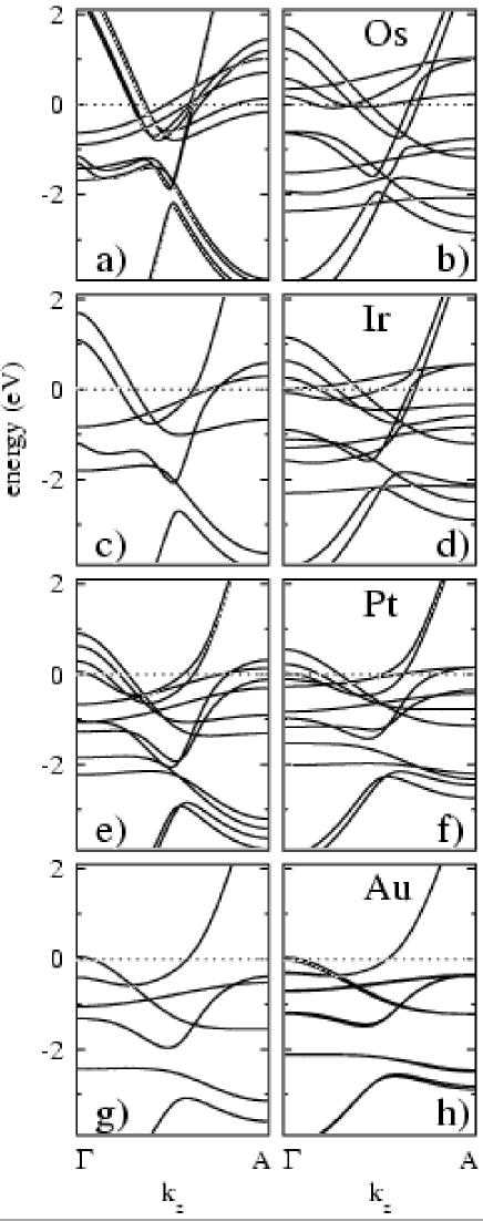
Figure 3: Band structures, along the wire direction, at two different bond lengths (the equilibrium one, and a larger of 2.8 Å) for each element. The Fermi energy is at zero. Band doubling (present in panels a, b, d, e, f, and h) indicates spin splitting due to magnetic order.

Some more detailed insight regarding the shape of the magnetic profiles can be gained by analyzing the band structures, and how they change as a function of bond length. Band structures for two different bond lengths, the equilibrium bond length, and a larger one of 2.8 Å, roughly representing two magnetic regimes, are shown in Fig. 3 for each of our four elements. The bands run from the zone center, $\Gamma$, to the zone edge, A, in the direction of the wire.

The character of the bands close to the Fermi level is of critical importance for the moment formation, and therefore we also show character-resolved bands, see Fig. 4. We found it useful to split up the $d$ character into $d_{z}$, $d_{xz}+d_{yz}$ and $d_{xy}+d_{x^{2}-y^{2}}$, and so, Fig 4 has four panels, displaying separately the $s$, $d_{z}$, $d_{xz}+d_{yz}$ and $d_{xy}+d_{x^{2}-y^{2}}$ characters of the bands. The vertical error bars, or “thickness”, of the bands indicate the relative character weight. The data in Fig 4 has been taken from a calculation for Pt. However, for the other metals, the relative weight of the orbitals for each band is qualitatively similar to the one shown. From Fig. 4, we see that almost all bands in the vicinity of the Fermi level have predominantly $d$ character. In fact, there are only two bands with some $s$ character crossing the Fermi level (see upper left panel in Fig. 4). Of these, the highest lying band crosses the Fermi level halfway between the zone center and zone edge. This band is almost purely $s$ at that crossing. For Ir, Os and Pt, this band actually crosses the Fermi level twice. However, the degree of $s$ character for this band diminishes rapidly as the reciprocal lattice vector approaches the zone center $\Gamma$, i.e., the second crossing is $d$-dominated, as is evident from Fig. 4. The second one of the two $s$-containing bands crosses the Fermi level close to the zone edge (A). At that point, it has some $s$ character, but is in fact dominated by $d_{z}$ character.

At $\Gamma$ and A, both of them critical points by symmetry, all band dispersions are horizontal, giving rise to very sharp band edge van Hove singularities, a feature due to the one-dimensionality of the systems. Since the bands have mostly $d$ character at the edges, the exchange energy gain will be rather large if a band spin-splits so that one of the spin-channel band edges ends up above the Fermi level, and the other one below. Strictly speaking, the spin-orbit coupling will mix the two spin channels so that, in general, an eigenvalue will have both majority and minority spin character. However, in the present calculations, this mixing is so small, typically just a few percent, that it is irrelevant for the qualitative discussion we make here. Thus, if a band edge ends up sufficiently near the Fermi level, we may expect a magnetic moment to develop. While apparently similar to the magnetization of the jellium wire, magnetism here is much more substantial, the $d$ states involving a much stronger Hund’s rule exchange. We now go through all four metals, starting with Os, analyzing how the band edges move as a function of bond length, and how this affects the magnetic state of the wires.

Os: The magnetism in the Os wire has two regimes, one for bond lengths below 2.6 Å, and one for bond lengths above this value. Below 2.6 Å, the magnetic moment actually decreases with increasing bond length. At the equilibrium bond length, only one band edge (of mostly $d_{z}$ character and some $s$ character), at A, has spin-split around the Fermi level (see panel a in Fig 3). This gives rise to a small moment of a few tenths of a $\mu_{B}$. As the bond length increases, this band edge moves downward, through the Fermi level, and the magnetic moment is killed off. At the same time, the band edges (at $\Gamma$ and A) of the rather flat $d_{xy}+d_{x^{2}-y^{2}}$ band come sufficiently close to the Fermi level, causing a large splitting (see panel b). This results in a rapid increase of the magnetic moment, creating the second, large-moment, magnetic regime.

Ir: With one more electron than Os, the bands of the Ir wire lie generally deeper. At the equilibrium bond length, the band edge responsible for the low-moment regime for Os lies well below the Fermi level and is inactive. With increased bond length, the A edge of the flat $d_{xy}+d_{x^{2}-y^{2}}$ band gradually sinks toward the Fermi level and eventually causes a large magnetic splitting. Thus, the whole magnetic regime in Ir is similar to the large-moment regime in Os.

Pt: In Pt, the very same flat $d_{xy}+d_{x^{2}-y^{2}}$ band leading to Hund’s rule magnetism in Os and Ir behaves here in the opposite way. At very small bond lengths (2.2 Å), this band is entirely occupied, and moves upwards (instead of downwards) with increased bond lengths. As the edge at A touches the Fermi level, a magnetic moment develops. Two other bands, a $d_{z^{2}}$-dominated one with band edge at A and a $d_{xz}+d_{yz}$-dominated one with band edge at $\Gamma$ are also important. They are just slightly higher in energy than the first band edge, and with increasing bond length, they move to lower energies. Thus, these three band edges become increasingly degenerate with stretching, and split around the Fermi level at 2.4 Å, causing a rapid increase in the magnetic moment.

Au: For Au, the $d$ bands causing the magnetism in Os, Ir, and Pt lie well below the Fermi level and cannot give rise to a magnetic moment. The magnetically active band edge is at $\Gamma$, and belongs to a band with relatively high dispersion and $d_{xz}+d_{yz}$ character. With increasing bond length, this band edge moves downward, and as it passes through the Fermi level it creates a small magnetic moment. As can be seen in Fig. 3, panel h, the spin splitting of the band edge is really very tiny, and the magnetism in Au is reminiscent of the magnetism of the jellium cylinder, i.e., a band-edge phenomenon rather than Hund’s rule driven spin polarization. Further stretching causes this edge to sink below the Fermi energy, and the magnetic moment consequently disappears. It is not clear at present whether this moment may be of any real physical significance.

III.3 Ballistic conductance channels

As seen from the above discussion of the nanowire band structures, spin-splitting of bands does alter the number of bands — or channels — $n$ crossing the Fermi level. By virtue of the Landauer formula

$$G=\frac{e^{2}}{h}\sum_{i}\tau_{i},$$ (1)

where $\tau_{i}$ is the transmission through channel $i$, the ballistic conductance measured has, in units of $\frac{1}{2}G_{0}=e^{2}/h$, precisely the number of bands $n$ crossing the Fermi level as its upper limit. Thus, the conductance through the wires should be affected by magnetism.

Fig. 5 shows how the number $n$ of conducting channels is influenced by nanowire spin-polarization and bond length. For Os and Pt in their magnetized state at the equilibrium bond length, $n$ is large, 11 and 8, respectively, against 12 and 10 in the nonmagnetic state. Magnetism has decreased the number of channels, but not dramatically so. Should all these channels transmit fully, a large ballistic conductance of $4G_{0}$ for Pt or $5.5G_{0}$ for Os would ensue, to be compared with nonmagnetic values of $5G_{0}$ and $6G_{0}$, respectively.

In reality however most of the open channels have $d$ character. While the conductance of the broad band $s$ channels is generally close to one owing to nearly complete transmission, that of the narrow band $d$ channels is much smaller, with a high reflection at the lead-wire junction, generally dependent on the detailed junction geometry. Of the conductance channels in these metals, two have $s$ character, both in the spin-polarized and nonmagnetic calculations, bringing an expected contribution close to $G_{0}$ to the total conductance. All the other channels have predominantly $d$ character. Their contribution to the conductance is therefore expected to be much smaller than $\frac{1}{2}G_{0}$ per channel. We may thus expect these wires to have a conductance above $G_{0}$ but well below $4G_{0}$ and $5.5G_{0}$, respectively. Since the scattering of the $d$ waves at the junctions depends highly on the geometry, whose details will change at every realization, we also expect the conductance histograms to exhibit peaks that could be both broad and poorly reproducible. For Ir, our calculations indicate that the conductance at the equilibrium bond length should lie between $G_{0}$ and $5G_{0}$. For these three metals, according to our calculations the number of conductance channels decreases — by and large — as the wire is stretched. However, the disappearing channels are always $d$-dominated.

Of the metals Os, Ir and Pt, measured conductance histograms have been published only for Pt so far. Smit et al.smit2002 find a large, broad peak centered around $1.5G_{0}$ and a smaller bump centered around $2.2G_{0}$. The conductance histograms reported by Yansonyanson_thesis are similar in structure, but the positions are shifted, to around $1.7G_{0}$ and $3G_{0}$. Rodrigues et al.rodrigues find a peak centered around $1.4G_{0}$, and in addition a peak at very low conductance, around $0.5G_{0}$.

In the Au wire, we find theoretically four open conductance channels. Two of these are $s$ dominated, just as for the other metals, and two are $d$ dominated. However, the $d$ channels are merely touching the Fermi level, and are therefore expected to have a very marginal effect on the conductance. Experimentally, gold nanowires yield a rather sharp peak between $0.9G_{0}$ and $G_{0}$, confirming that the $d$ influence is probably very small.

IV Conclusions

In conclusion, our calculations suggest that the Os, Ir, and Pt monatomic nanowires should exhibit spontaneous Hund’s rule superparamagnetism for values of the bond length at equilibrium or — in the case of Ir — slightly above. The energy gain connected with the magnetic state is small, less than 10 meV for Os and Pt at the equilibrium bond length. Au nanowires also theoretically magnetize, but the calculated energy gain is an order of magnitude smaller than for the other metals. From a methodological point of view, the spin-orbit coupling is found to be crucial for a correct description of the magnetic state, as is probably the use of all-electron techniques.bahn2001

How might this magnetism be detected experimentally? Merely measuring the conduction through the wire at one single temperture and magnetic field strength will most probably not give conclusive information regarding the magnetic state of the atoms in the wire, since the tranmission through $d$ channels is rather poor and vary greatly with geometry and can hardy be regarded as quantized. A key experiment would be to measure ballistic conductance as a function of temperature and of external magnetic field. At high temperature and zero field the nanowire should be nonmagnetic, due to fast fluctuations. High field and low temperature would take the nanowire to a magnetic, or in any case to a slowly fluctuating superparamagnetic regime. In this transition the number of conductance channels should diminish, and so should the conductance — even if not by very much. At sufficiently low temperatures, the conductance should definitely be field sensitive. Such a behavior would be a clear indication of a superparamagnetic state.

In some situations, more majority bands may cross the Fermi level than do minority bands, leading to partial spin-polarization of the transmitted electron current. If this current could be measured, it would be a very direct way of confirming the existence of a superparamagnetic state.

Fractional conductance peaks have been observed experimentally, for example the $\frac{1}{2}G_{0}$ peak reported by Ono for Ni,ono1999 and very recently by Rodrigues et al. for Co, Pd and Pt,rodrigues at room temperature and zero field. These results are intriguing, since we expect that the $s$ channel alone should yield a conductance larger than that. The peaks observed in Co, Pd, and Pt, centered around $\frac{1}{2}G_{0}$, are rather broad, which suggests that they might not be caused by one single fully transmitting spin-polarized channel, but perhaps by several poorly conducting channels. We discussed in previous work,smogunov1 a possibility to obtain conductance $G_{0}$ from a magnetic transition metal nanowire with a magnetization reversal occurring inside the nanowire. This could further drop to $\frac{1}{2}G_{0}$ in an asymmetrical situation, with a net prevalence of majority spins over minority spins. Although it is not inconceivable that this might occur in Co and Ni, we are unable to explain at the moment how that kind of state could be sustained in Pt, and by extension in Pd too, at the experimental conditions of zero field and room temperature. It would anyway be interesting to see the effect of cooling and of an external field on these results.

Figure 1: Total magnetic moments, both with spin-orbit coupling (FR) and without (SR), per atom as a function of bond length. The dashed vertical line points out the equilibrium bond length.

Figure 2: Bottom and top of the $s$ and $d$ bands as a function of bond length. The Fermi energy is at zero.

Figure 4: Character-resolved band structure for nonspinpolarized Pt, along the wire direction. The Fermi energy is at zero.

Figure 5: The number of open conductance channels as a function of bond length. FM = ferromagnetic calculation; NM = nonmagnetic calculation. The dashed vertical line points out the equilibrium bond length.

- (1) K. Kondo and K. Takayanagi, Science 289, 606 (2000).
- (2) V. Rodrigues, T. Fuhrer, and D. Ugarte, Phys. Rev. Lett. 85, 4124 (2000).
- (3) R. H. M. Smit et al., Phys. Rev. Lett. 87, 266102 (2001)
- (4) B. J. van Wees et al., Phys. Rev. Lett. 60, 848 (1988).
- (5) O. Gülseren, F. Ercolessi, and E. Tosatti, Phys. Rev. Lett. 80, 3775-3778 (1998).
- (6) E. Tosatti et al., Science 291, 288 (2001).
- (7) H. Ohnishi, Y. Kondo, and K. Takayanagi, Nature, 395, 780 (1998).
- (8) A. I. Yanson, et al., Nature 395, 783 (1998).
- (9) P. Gambardella et al., Nature 416, 301 (2002).
- (10) B. H. Hong et al., Science 294, 348 (2001).
- (11) N. Zabala, M. J. Puska, and R. M. Nieminen, Phys. Rev. Lett. 80, 3336 (1998); Comment and Reply, ibid. 82 3000 (1999).
- (12) In the case of Pt, we also performed antiferromagnetic calculations, but found this magnetic configuration to be unstable with respect to ferromagnetic ordering.
- (13) S. Blügel, Phys. Rev. Lett. 68 851 (1992).
- (14) J. Redinger, S. Blügel, and R. Podloucky, Phys. Rev. B 51, 13852 (1995).
- (15) D. Sanchez-Portal, et al., Phys. Rev. Lett. 83, 3884-3887 (1999).
- (16) J. A. Torres et al., Surf. Science 426, L441-L446 (1999).
- (17) P. Hohenberg and W. Kohn, Phys. Rev. 136, B864 (1964); W. Kohn and L. J. Sham, Phys. Rev. 140, A1133 (1965).
- (18) J. M. Wills, O. Eriksson, M. Alouani, and O. L. Price, in Electronic Structure and Physical Properties of Solids, edited by H. Dreyssé (Springer, Berlin, 2000).
- (19) J. P. Perdew, in Electronic Structure of Solids 1991, edited by P. Ziesche and H. Eschrig (Akademie Verlag, Berlin, 1991); J. P. Perdew, K. Burke, and M. Ernzerhof, Phys. Rev. Lett. 77, 3865 (1996); J. P. Perdew, K. Burke, and M. Ernzerhof, Phys. Rev. Lett. 78, 1396 (1997); Y. Zhang and W. Yang, Phys. Rev. Lett. 80, 890 (1998); J. P. Perdew, K. Burke, and M. Ernzerhof, Phys. Rev. Lett. 80, 891 (1998).
- (20) D. M. Ceperley and B. J. Alder, Phys. Rev. Lett. 45, 566 (1980); J. P. Perdew and A. Zunger, Phys. Rev. B23, 5048 (1981).
- (21) P. Blaha, K. Schwarz, and J. Luitz, computer code WIEN97 (Vienna University of Technology, Vienna, 1997), [Improved and updated UNIX version of the original copyrighted WIEN code, which was published by P. Blaha, K. Schwarz, P. Sorantin, and S. B. Trickey, Comput. Phys. Commun. 59, 339 (1990)].
- (22) S. R. Bahn and K. W. Jacobsen, Phys. Rev. Lett. 87, 266101 (2001).
- (23) L. De Maria and M. Springborg, Chem. Phys. Lett. 323, 293 (2000).
- (24) R. H. M. Smit et al., Nature 409, 906 (2002).
- (25) A. I. Yanson, Thesis, Universiteit Leiden, The Netherlands (2001).
- (26) V. Rodrigues, J. Bettini, P. C. Silva, and D. Ugarte, preprint.
- (27) T. Ono, Y. Ooka, H. Miyajima, and Y. Otani, Appl. Phys. Lett. 75, 1622 (1999).
- (28) A. Smogunov, A. Dal Corso, and E. Tosatti, Surf. Science 507, 609 (2002).