Estimating Mutual Information

Abstract

We present two classes of improved estimators for mutual information $M(X,Y)$, from samples of random points distributed according to some joint probability density $\mu(x,y)$. In contrast to conventional estimators based on binnings, they are based on entropy estimates from $k$-nearest neighbour distances. This means that they are data efficient (with $k=1$ we resolve structures down to the smallest possible scales), adaptive (the resolution is higher where data are more numerous), and have minimal bias. Indeed, the bias of the underlying entropy estimates is mainly due to non-uniformity of the density at the smallest resolved scale, giving typically systematic errors which scale as functions of $k/N$ for $N$ points. Numerically, we find that both families become exact for independent distributions, i.e. the estimator $\hat{M}(X,Y)$ vanishes (up to statistical fluctuations) if $\mu(x,y)=\mu(x)\mu(y)$. This holds for all tested marginal distributions and for all dimensions of $x$ and $y$. In addition, we give estimators for redundancies between more than 2 random variables. We compare our algorithms in detail with existing algorithms. Finally, we demonstrate the usefulness of our estimators for assessing the actual independence of components obtained from independent component analysis (ICA), for improving ICA, and for estimating the reliability of blind source separation.

I Introduction

Among the measures of independence between random variables, mutual information (MI) is singled out by its information theoretic background cover-thomas . In contrast to the linear correlation coefficient, it is sensitive also to dependencies which do not manifest themselves in the covariance. Indeed, MI is zero if and only if the two random variables are strictly independent. The latter is also true for quantities based on Renyi entropies renyi , and these are often easier to estimate (in particular if their order is 2 or some other integer $>2$). Nevertheless, MI is unique in its close ties to Shannon entropy and the theoretical advantages derived from this. Some well known properties of MI and some simple consequences thereof are collected in the appendix.

But it is also true that estimating MI is not always easy. Typically, one has a set of $N$ bivariate measurements, $z_{i}=(x_{i},y_{i}),\,i=1,\ldots N$, which are assumed to be iid (independent identically distributed) realizations of a random variable $Z=(X,Y)$ with density $\mu(x,y)$. Here, $x$ and $y$ can be either scalars or can be elements of some higher dimensional space. In the following we shall assume that the density is a proper smooth function, although we could also allow more singular densities. All we need is that the integrals written below exist in some sense. In particular, we will always assume that $0\log(0)=0$, i.e. we do not have to assume that densities are strictly positive. The marginal densities of $X$ and $Y$ are $\mu_{x}(x)=\int dy\mu(x,y)$ and $\mu_{y}(y)=\int dx\mu(x,y)$. The MI is defined as

$$I(X,Y)=\int\!\!\!\int dxdy\;\mu(x,y)\;\log{\mu(x,y)\over\mu_{x}(x)\mu_{y}(y)}\;.$$ (1)

The base of the logarithm determines the units in which information is measured. In particular, taking base two leads to information measured in bits. In the following, we always will use natural logarithms. The aim is to estimate $I(X,Y)$ from the set $\{z_{i}\}$ alone, without knowing the densities $\mu,\mu_{x}$, and $\mu_{y}$.

One of the main fields where MI plays an important role, at least conceptually, is independent component analysis (ICA) robe-ever ; hyvar2001 . In the ICA literature, very crude approximations to MI based on cumulant expansions are popular because of their ease of use. But they are valid only for distributions close to Gaussians and can mainly be used for ranking different distributions by interdependence, much less for estimating the actual dependences. Expressions obtained by entropy maximalization using averages of some functions of the sample data as constraints hyvar2001 are more robust, but are still very crude approximations. Finally, estimates based on explicit parameterizations of the densities might be useful but are not very efficient. More promising are methods based on kernel density estimators moon95 ; steuer02 . We will not pursue these here either, but we will comment on them in Sec. IV.A.

The most straightforward and widespread approach for estimating MI more precisely consists in partitioning the supports of $X$ and $Y$ into bins of finite size, and approximating Eq.(1) by the finite sum

$$I(X,Y)\approx I_{\rm binned}(X,Y)\equiv\sum_{ij}p(i,j)\log{p(i,j)\over p_{x}(i)p_{y}(j)}\;,$$ (2)

where $p_{x}(i)=\int_{i}dx\;\mu_{x}(x)$, $p_{y}(j)=\int_{j}dy\;\mu_{y}(y)$, and $p(i,j)=\int_{i}\int_{j}dxdy\;\mu(x,y)$ – and $\int_{i}$ means the integral over bin $i$. An estimator of $I_{\rm binned}(X,Y)$ is obtained by counting the numbers of points falling into the various bins. If $n_{x}(i)\;(n_{y}(j))$ is the number of points falling into the $i$-th bin of $X$ ($j$-th bin of $Y$), and $n(i,j)$ is the number of points in their intersection, then we approximate $p_{x}(i)\approx n_{x}(i)/N$, $p_{y}(j)\approx n_{y}(j)/N$, and $p(i,j)\approx n(i,j)/N$. It is easily seen that the r.h.s. of Eq.(2) indeed converges to $I(X,Y)$ if we first let $N\to\infty$ and then let all bin sizes tend to zero, if all densities exist as proper (not necessarily smooth) functions. If not, i.e. if the distributions are e.g. (multi-)fractal, this convergence might no longer be true. In that case, Eq.(2) would define resolution dependent mutual entropies which diverge in the limit of infinite resolution. Although the methods developed below could be adapted to apply also to that case, we shall not do this in the present paper.

The bin sizes used in Eq.(2) do not need to be the same for all bins. Optimized estimators fraser-swinney ; darbellay-vajda use indeed adaptive bin sizes which are essentially geared at having equal numbers $n(i,j)$ for all pairs $(i,j)$ with non-zero measure. While such estimators are much better than estimators using fixed bin sizes, they still have systematic errors which result on the one hand from approximating $I(X,Y)$ by $I_{\rm binned}(X,Y)$, and on the other hand by approximating (logarithms of) probabilities by (logarithms of) frequency ratios. The latter could be presumably minimized by using corrections for finite $n_{x}(i)$ resp. $n(i,j)$ grass88 . These corrections are in the form of asymptotic series which diverge for finite $N$, but whose first 2 terms improve the estimates in typical cases. The first correction term – which often is not sufficient – was taken into account in roulston99 ; steuer02 .

In the present paper we will not follow these lines, but rather estimate MI from $k$-nearest neighbour statistics. There exists an extensive literature on such estimators for the simple Shannon entropy

$$H(X)=-\int dx\mu(x)\log\mu(x),$$ (3)

dating back at least to dobrushin ; vasicek . But it seems that these methods have never been used for estimating MI. In vasicek ; dude-meul ; es ; ebrahimi ; correa ; tsyb-meul ; wiecz-grze it is assumed that $x$ is one-dimensional, so that the $x_{i}$ can be ordered by magnitude and $x_{i+1}-x_{i}\to 0$ for $N\to\infty$. In the simplest case, the estimator based only on these distances is

$$H(X)\approx{1\over N-1}\sum_{i=1}^{N-1}\log(x_{i+1}-x_{i})+\psi(1)-\psi(N)\;.$$ (4)

Here, $\psi(x)$ is the digamma function, $\psi(x)=\Gamma(x)^{-1}d\Gamma(x)/dx$. It satisfies the recursion $\psi(x+1)=\psi(x)+1/x$ and $\psi(1)=-C$ where $C=0.5772156\ldots$ is the Euler-Mascheroni constant. For large $x$, $\psi(x)\approx\log x-1/2x$. Similar formulas exist which use $x_{i+k}-x_{i}$ instead of $x_{i+1}-x_{i}$, for any integer $k<N$.

Although Eq.(4) and its generalizations to $k>1$ seem to give the best estimators of $H(X)$, they cannot be used for MI because it is not obvious how to generalize them to higher dimensions. Here we have to use a slightly different approach, due to koza-leon (see also grass85 ; somorjai86 ; the latter authors were only interested in fractal measures and estimating their information dimensions, but the basic concepts are the same as in estimating $H(X)$ for smooth densities).

Assume some metrics to be given on the spaces spanned by $X,Y$ and $Z=(X,Y)$. We can then rank, for each point $z_{i}=(x_{i},y_{i})$, its neighbours by distance $d_{i,j}=||z_{i}-z_{j}||$: $d_{i,j_{1}}\leq d_{i,j_{2}}\leq d_{i,j_{3}}\leq\ldots$. Similar rankings can be done in the subspaces $X$ and $Y$. The basic idea of koza-leon ; grass85 ; somorjai86 is to estimate $H(X)$ from the average distance to the $k$-nearest neighbour, averaged over all $x_{i}$. Details will be given in Sec.II. Mutual information could be obtained by estimating in this way $H(X)$, $H(Y)$ and $H(X,Y)$ separately and using cover-thomas

$$I(X,Y)=H(X)+H(Y)-H(X,Y)\;.$$ (5)

But this would mean that the errors made in the individual estimates would presumably not cancel, and therefore we proceed differently.

Indeed we will present two slightly different algorithms, both based on the above idea. Both use for the space $Z=(X,Y)$ the maximum norm,

$$||z-z^{\prime}||=\max\{||x-x^{\prime}||,||y-y^{\prime}||\},$$ (6)

while any norms can be used for $||x-x^{\prime}||$ and $||y-y^{\prime}||$ (they need not be the same, as these spaces could be completely different). Let us denote by $\epsilon(i)/2$ the distance from $z_{i}$ to its $k$-th neighbour, and by $\epsilon_{x}(i)/2$ and $\epsilon_{y}(i)/2$ the distances between the same points projected into the $X$ and $Y$ subspaces. Obviously, $\epsilon(i)=\max\{\epsilon_{x}(i),\epsilon_{y}(i)\}$.

In the first algorithm, we count the number $n_{x}(i)$ of points $x_{j}$ whose distance from $x_{i}$ is strictly less than $\epsilon(i)/2$, and similarly for $y$ instead of $x$. This is illustrated in Fig. 1a. Notice that $\epsilon(i)$ is a random (fluctuating) variable, and therefore also $n_{x}(i)$ and $n_{y}(i)$ fluctuate. We denote by $\langle\ldots\rangle$ averages both over all $i\in[1,\ldots N]$ and over all realizations of the random samples,

$$\langle\ldots\rangle=N^{-1}\sum_{i=1}^{N}{\sf E}[\ldots(i)]\;.$$ (7)

The estimate for MI is then

$$I^{(1)}(X,Y)=\psi(k)-\langle\psi(n_{x}+1)+\psi(n_{y}+1)\rangle+\psi(N).$$ (8)

Figure 1: Panel (a): Determination of $\epsilon(i)$, $n_{x}(i)$ and $n_{y}(i)$ in the first algorithm, for $k=1$ and some fixed $i$. In this example, $n_{x}(i)=5$ and $n_{y}(i)=3$.
Panels (b),(c): Determination of $\epsilon_{x}(i)$, $\epsilon_{y}(i)$, $n_{x}(i)$ and $n_{y}(i)$ in the second algorithm. Panel (b) shows a case where $\epsilon_{x}(i)$ and $\epsilon_{y}(i)$ are determined by the same point, while panel (c) shows a case where they are determined by different points.

Alternatively, in the second algorithm, we replace $n_{x}(i)$ and $n_{y}(i)$ by the number of points with $||x_{i}-x_{j}||\leq\epsilon_{x}(i)/2$ and $||y_{i}-y_{j}||\leq\epsilon_{y}(i)/2$ (see Figs. 1b and 1c). The estimate for MI is then

$$I^{(2)}(X,Y)=\psi(k)-1/k-\langle\psi(n_{x})+\psi(n_{y})\rangle+\psi(N).$$ (9)

The derivations of Eqs.(8) and (9) will be given in Sec.II. There we will also give formulas for generalized redundancies in higher dimensions,

$$I(X_{1},X_{2},\ldots X_{m}) = H(X_{1})+H(X_{2})+\ldots+H(X_{m})$$ (10)

$$- H(X_{1},X_{2},\ldots X_{m}).$$

In general, both formulas give very similar results. For the same $k$, Eq.(8) gives slightly smaller statistical errors (because $n_{x}(i)$ and $n_{y}(i)$ tend to be larger and have smaller relative fluctuations), but have larger systematic errors. The latter is only severe if we are interested in very high dimensions where $\epsilon(i)$ tends typically to be much larger than the marginal $\epsilon_{x_{j}}(i)$. In that case the second algorithm seems preferable. Otherwise, both can be used equally well.

A systematic study of the performance of Eqs.(8) and (9) and comparison with previous algorithms will be given in Sec.III. Here we will just show results of $I^{(2)}(X,Y)$ for Gaussian distributions. Let $X$ and $Y$ be Gaussians with zero mean and unit variance, and with covariance $r$. In this case $I(X,Y)$ is known exactly darbellay-vajda ,

$$I_{\rm Gauss}(X,Y)=-{1\over 2}\log(1-r^{2})\;.$$ (11)

In Fig. 2 we show the errors $I^{(2)}(X,Y)-I_{\rm Gauss}(X,Y)$ for various values of $r$, obtained from a large number (typically $10^{5}-10^{7}$) of realizations. We show only results for $k=1$, plotted against $1/N$. Results for $k>1$ are similar. To a first approximation $I^{(1)}(X,Y)$ and $I^{(2)}(X,Y)$ depend only on the ratio $k/N$.

The most conspicuous feature seen in Fig. 2, apart from the fact that indeed $I^{(2)}(X,Y)-I_{\rm Gauss}(X,Y)\to 0$ for $N\to\infty$, is that the systematic error is compatible with zero for $r=0$, i.e. when the two Gaussians are uncorrelated. We checked this with high statistics runs for many different values of $k$ and $N$ (a priori one should expect that systematic errors become large for very small $N$), and for many more distributions (exponential, uniform, …). In all cases we found that both $I^{(1)}(X,Y)$ and $I^{(2)}(X,Y)$ become exact for independent variables. Moreover, the same seems to be true for higher order redundancies. We thus have the

Conjecture: Eqs.(8) and (9) are exact for independent $X$ and $Y$, i.e. $I^{(1)}(X,Y)=I^{(2)}(X,Y)=0$ if and only if $I(X,Y)=0$.

We have no proof for this very surprising result. We have numerical indications that moreover

$${|I^{(1,2)}(X,Y)-I(X,Y)|\over I(X,Y)}\leq{\rm const}$$ (12)

as $X$ and $Y$ become more and more independent, but this is much less clean and therefore much less sure.

In Sec.II we shall give formal arguments for our estimators, and for generalizations to higher dimensions. Detailed numerical results for cases where the exact MI is known will be given in Sec.III. In Sec.IV.A we give two preliminary applications to gene expression data and to ICA. Conclusions are drawn in the last section, Sec.V. Finally, some general aspects of MI are recalled in an appendix.

Figure 2: Estimates of $I^{(2)}(X,Y)-I_{\rm exact}(X,Y)$ for Gaussians with unit variance and covariances $r=0.9,0.6,0.3$, and 0.0 (from top to bottom), plotted against $1/N$. In all cases $k=1$. The number of realizations is $>2\times 10^{6}$ for $N<=1000$, and decreases to $\approx 10^{5}$ for $N=40,000$. Error bars are smaller than the sizes of the symbols.

II Formal Developments

II.1 Kozachenko - Leonenko Estimate for Shannon Entropies

We first review the derivation of the Shannon entropy estimate grass85 ; somorjai86 ; koza-leon ; victor , since the estimators for MI are obtained by very similar arguments.

Let $X$ be a continuous random variable with values in some metric space, i.e. there is a distance function $||x-x^{\prime}||$ between any two realizations of $X$, and let the density $\mu(x)$ exist as a proper function. Shannon entropy is defined as

$$H(X)=-\int dx\mu(x)\log\mu(x)\;,$$ (13)

where “log” will always mean natural logarithm so that information is measured in natural units. Our aim is to estimate $H(X)$ from a random sample $(x_{1}\ldots x_{N})$ of $N$ realizations of $X$.

The first step is to realize that Eq.(13) can be understood (up to the minus sign) as an average of $\log\mu(x)$. If we had unbiased estimators $\widehat{\log\mu(x)}$ of the latter, we would have an unbiased estimator

$$\hat{H}(X)=-N^{-1}\sum_{i=1}^{N}\widehat{\log\mu(x_{i})}\;.$$ (14)

In order to obtain the estimate $\widehat{\log\mu(x_{i})}$, we consider the probability distribution $P_{k}(\epsilon)$ for the distance between $x_{i}$ and its $k$-th nearest neighbour. The probability $P_{k}(\epsilon)d\epsilon$ is equal to the chance that there is one point within distance $r\in[\epsilon/2,\epsilon/2+d\epsilon/2]$ from $x_{i}$, that there are $k-1$ other points at smaller distances, and that $N-k-1$ points have larger distances from $x_{k}$. Let us denote by $p_{i}$ the mass of the $\epsilon$-ball centered at $x_{i}$, $p_{i}(\epsilon)=\int_{||\xi-x_{i}||<\epsilon/2}d\xi\mu(\xi)$. Using the trinomial formula we obtain

$$P_{k}(\epsilon)d\epsilon = {(N-1)!\over 1!(k-1)!(N-k-1)!}\;\times$$ (15)

$$\times {dp_{i}(\epsilon)\over d\epsilon}d\epsilon\;\times\ p_{i}^{k-1}\times(1-p_{i})^{N-k-1}$$

or

$$P_{k}(\epsilon)=k{N-1\choose k}\;{dp_{i}(\epsilon)\over d\epsilon}\;p_{i}^{k-1}(1-p_{i})^{N-k-1}\;.$$ (16)

One easily checks that this is correctly normalized, $\int d\epsilon P_{k}(\epsilon)=1$. Similarly, one can compute the expectation value of $\log p_{i}(\epsilon)$

$${\sf E}(\log p_{i}) = \int_{0}^{\infty}d\epsilon\;P_{k}(\epsilon)\log p_{i}(\epsilon)$$ (17)

$$= k{N-1\choose k}\;\int_{0}^{1}dp\;p^{k-1}(1-p)^{N-k-1}\log p$$

$$= \psi(k)-\psi(N)\;,$$

where $\psi(x)$ is the digamma function. The expectation is taken here over the positions of all other $N-1$ points, with $x_{i}$ kept fixed. An estimator for $\log\mu(x)$ is then obtained by assuming that $\mu(x)$ is constant in the entire $\epsilon$-ball. The latter gives

$$p_{i}(\epsilon)\approx c_{d}\epsilon^{d}\mu(x_{i})\;.$$ (18)

where $d$ is the dimension of $x$ and $c_{d}$ is the volume of the $d$-dimensional unit ball. For the maximum norm one has simply $c_{d}=1$, while $c_{d}=\pi^{d/2}/\Gamma(1+d/2)/2^{d}$ for Euclidean norm.

Using Eqs.(17) and (18) one obtains

$$\log\mu(x_{i})\approx\psi(k)-\psi(N)-d\;{\sf E}(\log\epsilon)-\log c_{d}\;,$$ (19)

which finally leads to

$$\hat{H}(X)=-\psi(k)+\psi(N)+\log c_{d}+{d\over N}\sum_{i=1}^{N}\log\epsilon(i)$$ (20)

where $\epsilon(i)$ is twice the distance from $x_{i}$ to its $k$-th neighbour.

From the derivation it is obvious that Eq.(20) would be unbiased, if the density $\mu(x)$ were strictly constant. The only approximation is in Eq.(18). For points on a torus (e.g. when $x$ is a phase) with a strictly positive density one can easily estimate the leading corrections to Eq.(18) for large $N$. One finds that they are $O(1/N^{2})$ and that they scale, for large $k$ and $N$, as $\sim(k/N)^{2}$. In most other cases (including e.g. Gaussians and uniform densities in bounded domains with a sharp cut-off) it seems numerically that the error is $\sim k/N$ or $\sim k/N\log(N/k)$.

II.2 Mutual Informations: Estimator $I^{(1)}(X,Y)$

Let us now consider the joint random variable $Z=(X,Y)$ with maximum norm. Again we take one of the $N$ points $z_{i}$ and consider the distance $\epsilon/2$ to its $k$-th neighbour. Again this is a random variable with distribution given by Eq.(16). Also Eq.(17) holds without changes. The first difference to the previous subsection is in Eq.(18), where we have to replace $d$ by $d_{Z}=d_{X}+d_{Y}$, $c_{d}$ by $c_{d_{X}}c_{d_{Y}}$, and of course $x_{i}$ by $z_{i}=(x_{i},y_{i})$. With these modifications we obtain therefore

$$\hat{H}(X,Y) = \psi(k)-\psi(N)-\log(c_{d_{X}}c_{d_{Y}})$$ (21)

$$- {d_{X}+d_{Y}\over N}\sum_{i=1}^{N}\log\epsilon(i)\;.$$

In order to obtain $I(X,Y)$, we have to subtract this from estimates for $H(X)$ and $H(Y)$. For the latter, we could use Eq.(20) directly with the same $k$. But this would mean that we would effectively use different distance scales in the joint and marginal spaces. For any fixed $k$, the distance to the $k$-th neighbour in the joint space will be larger than the distances to the neighbours in the marginal spaces. Since the bias in Eq.(20) from the non-uniformity of the density depends of course on these distances, the biases in $\hat{H}(X)$, $\hat{H}(Y)$, and in $\hat{H}(X,Y)$ would not cancel.

To avoid this, we notice that Eq.(20) holds for any value of $k$, and that we do not have to choose a fixed $k$ when estimating the marginal entropies. Assume, as in Fig. 1a, that the $k$-th neighbour of $x_{i}$ is on one of the vertical sides of the square of size $\epsilon(i)$. In this case, if there are altogether $n_{x}(i)$ points within the vertical lines $x=x_{i}\pm\epsilon(i)/2$, then $\epsilon(i)/2$ is the distance to the $(n_{x}(i)+1)-$st neighbour of $x_{i}$, and

$$\hat{H}(X) = {1\over N}\sum_{i=1}^{N}\psi(n_{x}(i)+1)-\psi(N)$$ (22)

$$- \log c_{d_{X}}-{d_{X}\over N}\sum_{i=1}^{N}\log\epsilon(i)\;.$$

For the other direction (the $y$ direction in Fig. 1a) this is not exactly true, i.e. $\epsilon(i)$ is not exactly equal to twice the distance to the $(n_{y}(i)+1)-$st neighbour, if $n_{y}(i)$ is analogously defined as the number of points with $||y_{j}-y_{i}||<\epsilon(i)/2$. Nevertheless we can consider Eq.(22) also as a good approximation for $H(Y)$, if we replace everywhere $X$ by $Y$ in its right hand side (this approximation becomes exact when $n_{y}(i)\to\infty$, and thus also when $N\to\infty$). If we do this, subtracting $\hat{H}(X,Y)$ from $\hat{H}(X)+\hat{H}(Y)$ leads directly to Eq.(8).

These arguments can be easily extended to $m$ random variables and lead to

$$I^{(1)}(X_{1},X_{2},\ldots X_{m}) = \psi(k)+(m-1)\psi(N)$$

$$- \langle\psi(n_{x_{1}})+\psi(n_{x_{2}})+\ldots\psi(n_{x_{m}})\rangle\;.$$

II.3 Mutual Informations: Estimator $I^{(2)}(X,Y)$

The main drawback of the above derivation is that the Kozachenko-Leonenko estimator is used correctly in only one marginal direction. This seems unavoidable if one wants to stick to “balls”, i.e. to (hyper-)cubes in the joint space. In order to avoid it we have to switch to (hyper-)rectangles.

Let us first discuss the case of two marginal variables $X$ and $Y$, and generalize later to $m$ variables $X_{1},\ldots X_{m}$. As illustrated in Figs. 1b and 1c, there are two cases to be distinguished (all other cases, where more points fall onto the boundaries $x_{i}\pm\epsilon_{x}(i)/2$ and $y_{i}\pm\epsilon_{y}(i)/2$, have zero probability; see however the third paragraph of Sec.III): Either the two sides $\epsilon_{x}(i)$ and $\epsilon_{y}(i)$ are determined by the same point (Fig. 1b), or by different points (Fig. 1c). In either case we have to replace $P_{k}(\epsilon)$ by a 2-dimensional density,

$$P_{k}(\epsilon_{x},\epsilon_{y})=P_{k}^{(b)}(\epsilon_{x},\epsilon_{y})+P_{k}^{(c)}(\epsilon_{x},\epsilon_{y})$$ (24)

with

$$P_{k}^{(b)}(\epsilon_{x},\epsilon_{y})={N-1\choose k}\;{d^{2}[q_{i}^{k}]\over d\epsilon_{x}d\epsilon_{y}}\;(1-p_{i})^{N-k-1}$$ (25)

and

$$P_{k}^{(c)}(\epsilon_{x},\epsilon_{y})=(k-1){N-1\choose k}\;{d^{2}[q_{i}^{k}]\over d\epsilon_{x}d\epsilon_{y}}\;(1-p_{i})^{N-k-1}\;.$$ (26)

Here, $q_{i}\equiv q_{i}(\epsilon_{x},\epsilon_{y})$ is the mass of the rectangle of size $\epsilon_{x}\times\epsilon_{y}$ centered at $(x_{i},y_{i})$, and $p_{i}$ is as before the mass of the square of size $\epsilon=\max\{\epsilon_{x},\epsilon_{y}\}$. The latter is needed since by using the maximum norm we guarantee that there are no points in this square which are not inside the rectangle.

Again we verify straightforwardly that $P_{k}$ is normalized, while we have now instead of Eq.(17)

$${\sf E}(\log q_{i}) = \int\!\!\!\!\int_{0}^{\infty}d\epsilon_{x}d\epsilon_{y}P_{k}(\epsilon_{x},\epsilon_{y})\log q_{i}(\epsilon_{x},\epsilon_{y})$$ (27)

$$= \psi(k)-1/k-\psi(N)\;.$$

Denoting now by $n_{x}(i)$ and $n_{y}(i)$ the number of points with distance less or equal to $\epsilon_{x}(i)/2$ resp. $\epsilon_{y}(i)/2$, we arrive at Eq.(9).

For the generalization to $m$ variables we have to consider $m$-dimensional densities $P_{k}(\epsilon_{x_{1}},\ldots\epsilon_{x_{m}})$. The number of distinct cases (analogous to the two cases shown in Figs. 1b and 1c) proliferates as $m$ grows, but fortunately we do not have to consider all these cases explicitly. One sees easily that each of them contributes to $P_{k}$ a term

$$\propto{d^{m}[q_{i}^{k}]\over d\epsilon_{x_{1}}\ldots d\epsilon_{x_{m}}}\;(1-p_{i})^{N-k-1}$$ (28)

The direct calculation of the proportionality factors would be extremely tedious (we did it for $m=3$), but it can be avoided by simply demanding that the sum is correctly normalized. This gives

$$P_{k}(\epsilon_{x_{1}},\ldots\epsilon_{x_{m}}) = k^{m-1}{N-1\choose k}{d^{m}[q_{i}^{k}]\over d\epsilon_{x_{1}}\ldots d\epsilon_{x_{m}}}\times\;$$ (29)

$$\times (1-p_{i})^{N-k-1}\;.$$

Calculating again ${\sf E}(\log q_{i})=\psi(k)-(m-1)/k-\psi(N)$ analytically and approximating the density by a constant inside the hyper-rectangle, we obtain finally

$$I^{(2)}(X_{1},X_{2},\ldots X_{m}) = \psi(k)-(m-1)/k$$

$$+ (m-1)\psi(N)$$

$$- \langle\psi(n_{x_{1}})+\psi(n_{x_{2}})+\ldots\psi(n_{x_{m}})\rangle\;.$$

Before leaving this section, we should mention that we slightly cheated in deriving $I^{(2)}(X,Y)$ (and its generalization to $m>2$). Assume that in a particular realization we have $\epsilon_{x}(i)<\epsilon_{y}(i)$, as in Fig. 1b,c. In that case we know that there cannot be any point in the two rectangles $[x_{i}-\epsilon_{y}(i)/2,x_{i}-\epsilon_{x}(i)/2]\times[y_{i}-\epsilon_{y}(i)/2,y_{i}+\epsilon_{y}(i)/2]$ and $[x_{i}+\epsilon_{x}(i)/2,x_{i}+\epsilon_{y}(i)/2]\times[y_{i}-\epsilon_{y}(i)/2,y_{i}+\epsilon_{y}(i)/2]$ (see Fig. 3). While we have taken this correctly into account when estimating $H(X,Y)$ (where it was crucial), we have neglected it in $H(X)$ and $H(Y)$. There, the corrections are $O(1/n_{x})$ and $O(1/n_{y})$, and should vanish for $N\to\infty$. It could be that their net effect vanishes, because they contribute with opposite signs to $H(X)$ and $H(Y)$. But we have no proof for it. Anyhow, due to the approximation of constant density within each rectangle we cannot expect our estimates to be exact for finite $N$, and any justification ultimately relies on numerics.

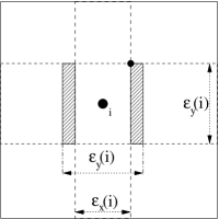
Figure 3: There cannot be any points inside the shaded rectangles. For method 2, this means that the estimates of the marginal entropy $H(X)$ ($H(Y)$) should be modified, since part of the area outside (inside) the stripe of with $\epsilon_{x}$ ($\epsilon_{y}$) is forbidden. This is neglected in Eq.(9).

III Implementation and Results

III.1 Some Implementation Details

Mutual information is invariant under reparametrization of the marginal variables. If $X^{\prime}=F(X)$ and $Y^{\prime}=G(Y)$ are homeomorphisms, then $I(X,Y)=I(X^{\prime},Y^{\prime})$ (see appendix). This is in contrast to $H(X)$ which changes in general under a homeomorphism. This can be used to rescale both variables first to unit variance. In addition, if the distributions are very skewed and/or rough, it might be a good idea to transform them such as to become more uniform (or at least single-humped and more or less symmetric). Although this is not required, strictly spoken, it will in general reduce errors. One example is the gamma-exponential distribution in 2 variables, $\mu(x,y)=x^{\theta}\exp(-x-xy)/\Gamma(\theta)$ for $x,y>0$ darb-vajd2000 , when $\theta<1$. For $\theta\to 0$, the marginal distributions develop $1/x$ resp. $1/y$ singularities (for $x\to 0$ and for $y\to\infty$, respectively), and the joint distribution is non-zero only in a very narrow region near the two axes. In this case our algorithm failed when applied directly, but it gave excellent results after transforming the variables to $x^{\prime}=\log x$ and $y^{\prime}=\log y$.

When implemented straightforwardly, the algorithm spends most of the CPU time for searching neighbours. In the most naive version, we need two nested loops through all points which gives a CPU time $O(N^{2})$. While this is acceptable for very small data sets (say $N\leq 300$), fast neighbour search algorithms are needed when dealing with larger sets. Let us assume that $X$ and $Y$ are scalars. An algorithm with complexity $O(N\sqrt{k\;N})$ is then obtained by first ranking the $x_{i}$ by magnitude (this can be done by any sorting algorithm such as quicksort), and co-ranking the $y_{i}$ with them numrec . Nearest neighbours of $(x_{i},y_{i})$ can then be obtained by searching $x$-neighbours on both sides of $x_{i}$ and verifying that their distance in $y$ direction is not too large. Neighbours in the marginal subspaces are found even easier by ranking both $x_{i}$ and $y_{i}$. Most results in this paper were obtained by this method which is suitable for $N$ up to a few thousands. The fastest (but also most complex) algorithm is obtained by using grids (‘boxes’) grass90 ; tisean . Indeed, we use three grids: A 2-dimensional one with box size $O(\sqrt{k/N})$ and two 1-dimensional ones with box sizes $O(1/N)$. First the $k$ neighbours in 2-d space are searched using the 2-d grid, then the boxes at distances $\pm\epsilon$ from the central point are searched in the 1-d grids to find $n_{x}$ and $n_{y}$. If the distributions are smooth, this leads to complexity $O(\sqrt{k}N)$. The last algorithm is comparable in speed to the algorithm of darbellay-vajda . For all three versions of our algorithm it costs only little additional CPU time if one evaluates, together with $I(X,Y)$ for some $k>1$, also the estimators for smaller $k$.

Empirical data usually are obtained with few (e.g. 12 or 16) binary digits, which means that many points in a large set may have identical coordinates. In that case the numbers $n_{x}(i)$ and $n_{y}(i)$ need no longer be unique (the assumption of continuously distributed points is violated). If no precautions are taken, any code based on nearest neighbour counting is then bound to give wrong results. The simplest way out of this dilemma is to add very low amplitude noise to the data ($\approx 10^{-10}$, say, when working with double precision) which breaks this degeneracy. We found this to give satisfactory results in all cases.

Often, MI is estimated after rank ordering the data, i.e. after replacing the coordinate $x_{i}$ by the rank of the $i$-th point when sorted by magnitude. This is equivalent to applying a monotonic transformation $x\to x^{\prime},\;y\to y^{\prime}$ to each coordinate which leads to a strictly uniform empirical density, $\mu^{\prime}_{x}(x^{\prime})=\mu^{\prime}_{y}(x^{\prime})=(1/N)\sum_{i=1}^{N}\delta(x^{\prime}-i)$. For $N\to\infty$ and $k\gg 1$ this clearly leaves the MI estimate invariant. But it is not obvious that it leaves invariant also the estimates for finite $k$, since the transformation is not smooth at the smallest length scale. We found numerically that rank ordering gives correct estimates also for small $k$, if the distance degeneracies implied by it are broken by adding low amplitude noise as discussed above. In particular, both estimators still gave zero MI for independent pairs. Although rank ordering can reduce statistical errors, we did not apply it in the following tests, and we did not study in detail the properties of the resulting estimators.

III.2 Results: Two-Dimensional Distributions

We shall first discuss applications of our estimators to correlated Gaussians, mainly because we can in this way most easily compare with analytic results and with previous numerical analyses. In all cases we shall deal with Gaussians of unit variance and zero mean. For $m$ such Gaussians with covariance matrix $\sigma_{ik}\;i,k=1\ldots m$, one has

$$I(X_{1},\ldots X_{m})=-{1\over 2}\log({\rm det}(\sigma))\;.$$ (31)

For $m=2$ and using the notation $r=\sigma_{XY}$, this gives Eq.(11).

Figure 4: Mutual information estimates $I^{(1)}(X,Y)$ (left panel) and $I^{(2)}(X,Y)$ (right panel) for Gaussian deviates with unit variance and covariance $r=0.9$, plotted against $k/N$ (left panel) resp. $(k-1/2)/N$ (right panel). Each curve corresponds to a fixed value of $N$, with $N=125,250,500,1000,2000,4000,10000$ and $20000$, from bottom to top. Error bars are smaller than the size of the symbols. The dashed line indicates the exact value $I(X,Y)=0.830366$.

First results for $I^{(2)}(X,Y)$ with $k=1$ were already shown in Fig. 2. Results obtained with $I^{(1)}(X,Y)$ are very similar and would indeed be hard to distinguish on this figure. In Fig. 4 we compare values of $I^{(1)}(X,Y)$ (left panel) with those for $I^{(2)}(X,Y)$ (right panel) for different values of $N$ and for $r=0.9$. The horizontal axes show $k/N$ (left) and $(k-1/2)/N$ (right). Except for very small values of $k$ and $N$, we observe scaling of the form

$$I^{(1)}(X,Y)\approx\Phi({k\over N})\;,\quad I^{(2)}(X,Y)\approx\Phi({k-1/2\over N})\;.$$ (32)

This is a general result and is found also for other distributions. The scaling with $k/N$ of $I^{(1)}(X,Y)$ results simply from the fact that the number of neighbours within a fixed distance would scale $\propto N$, if there were no statistical fluctuations. For large $k$ these fluctuations should become irrelevant, and thus the MI estimate should depend only on the ratio $k/N$. For $I^{(2)}(X,Y)$ this argument has to be slightly modified, since the smaller one of $\epsilon_{x}$ and $\epsilon_{y}$ is determined (for large $k$ where the situation illustrated in Fig. 1c dominates over that in Fig. 1b) by $k-1$ instead of $k$ neighbours.

The fact that $I^{(2)}(X,Y)$ for a given value of $k$ is between $I^{(1)}(X,Y)$ for $k-1$ and $I^{(1)}(X,Y)$ for $k$ is also seen from the variances of the estimates. In Fig. 5 we show the standard deviations, again for covariance $r=0.9$. These statistical errors depend only weakly on $r$. For $r=0$ they are roughly 10% smaller. As seen from Fig. 5, the errors of $I^{(2)}(X,Y;k)$ are roughly half-way between those of $I^{(1)}(X,Y;k-1)$ and $I^{(1)}(X,Y;k)$. They scale roughly as $\sim\sqrt{N}$, except for very large $k/N$. Their dependence on $k$ does not follow a simple scaling law. The fact that statistical errors increase when $k$ decreases is intuitively obvious, since then the width of the distribution of $\epsilon$ increases too. Qualitatively the same dependence of the errors was observed also for different distributions. For practical applications, it means that one should use $k>1$ in order to reduce statistical errors, but too large values of $k$ should be avoided since then the increase of systematic errors outweighs the decrease of statistical ones. We propose to use typically $k=2$ to 4, except when testing for independence. In the latter case we do not have to worry about systematic errors, and statistical errors are minimized by taking $k$ to be very large (up to $k\approx N/2$, say).

Figure 5: Standard deviations of the estimates $I^{(1)}(X,Y)$ ($+$) and $I^{(2)}(X,Y)$ ($\times$) for Gaussian deviates with unit variance and covariance $r=0.9$, multiplied by $\sqrt{N}$ and plotted against $k$ ($I^{(1)}(X,Y)$) resp. $k-1/2$ ($I^{(2)}(X,Y)$). Each curve corresponds to a fixed value of $N$, with $N=125,250,500,1000,2000,4000,10000$ and $20000$, from bottom to top.

The above shows that $I^{(1)}(X,Y)$ and $I^{(2)}(X,Y)$ behave very similar. Also CPU times needed to estimate them are nearly the same. In the following, we shall only show data for one of them, understanding that everything holds also for the other, unless the opposite is said explicitly.

For $N\to\infty$, the systematic errors tend to zero, as they should. From Figs. 2 and 4 one might conjecture that $I^{(1,2)}(X,Y)-I_{\rm exact}(X,Y)\sim N^{-1/2}$, but this is not true. Plotting this difference on a double logarithmic scale (Fig. 6), we see a scaling $\sim N^{-1/2}$ for $N\approx 10^{3}$, but faster convergence for larger $N$. It can be fitted by a scaling $\sim 1/N^{0.85}$ for the largest values of $N$ reached by our simulations, but the true asymptotic behaviour is presumably just $\sim 1/N$.

Figure 6: Systematic error $I^{(2)}(X,Y)-I_{\rm exact}(X,Y)$ for $k=3$ plotted against $N$ on log-log scale, for $r=0.9$. The dashed lines are $\propto N^{-0.5}$ and $\propto N^{-0.85}$.

As said in the introduction, the most surprising feature of our estimators is that they seem to be exact for independent random variables $X$ and $Y$. In Fig. 7 we show how the relative systematic errors behave for Gaussians when $r\to 0$. More precisely, we show $I^{(1,2)}(X,Y)/I^{(1,2)}_{\rm exact}(X,Y)$ for $k=1$, plotted against $N$ for four different values of $r$. Obviously these data converge, when $r\to 0$, to a finite function of $N$. We have observed the same also for other distributions, which leads to a conjecture stronger than the conjecture made in the introduction: Assume that we have a one-parameter family of 2-d distributions with densities $\mu(x,y;r)$, with $r$ being a real-valued parameter. Assume also that $\mu$ factorizes for $r=r_{0}$, and that it depends smoothly on $r$ in the vicinity of $r_{0}$, with $\partial\mu(x,y;r)/\partial r$ finite. Then we propose that for many distributions (although not for all!)

$$I^{(1,2)}(X,Y)/I_{\rm exact}(X,Y)\to F(k,N)$$ (33)

for $r\to r_{0}$, with some function $F(k,N)$ which is close to 1 for all $k$ and all $N\gg 1$, and which converges to 1 for $N\to\infty$. We have not found a general criterion for which families of distributions we should expect Eq.(33).

Figure 7: Ratios $I^{(2)}(X,Y)/I_{\rm exact}(X,Y)$ for $k=1$ plotted against $1/N$, for 4 different values of $r$.

The most precise and efficient previous algorithm for estimating MI is the one of Darbellay & Vajda darbellay-vajda . As far as speed is concerned, it seems to be faster than the present one, which might however be due to a more efficient implementation. In any case, also with the present algorithm we were able to obtain extremely high statistics on work stations within reasonable CPU times. To compare our statistical and systematic errors with those of darbellay-vajda , we have used the code basic.exe from http://siprint.utia.cas.cz/timeseries/. We used the parameter settings recommended in its description.

This code provides an estimate of the statistical error, even if only one data set is provided. When running it with many (typically $\approx 10^{4}$) data sets, we found that these error bars are always underestimated, sometimes by rather large margins. This seems to be due to occasional outliers which point presumably to some numerical instability. Unfortunately, having no source code we could not pin down the troubles. In Fig. 8 we compare the statistical errors provided by the code of darbellay-vajda , the errors obtained from the variance of the output of this code, and the error obtained from $I^{(2)}(X,Y)$ with $k=3$. We see that the latter is larger than the theoretical error from darbellay-vajda , but smaller than the actual error. For Gaussians with smaller correlation coefficients the statistical errors of darbellay-vajda decrease strongly with $r$, because the partitionings are followed to less and less depth. But, as we shall see, this comes with a risk for systematic errors.

Figure 8: Statistical errors (1 standard deviation) for Gaussian deviates with $r=0.9$, plotted against $N$. Results from $I^{(2)}(X,Y))$ for $k=1$ (full line) are compared to theoretically predicted (dashed) and actually measured (dotted line) errors from darbellay-vajda .

Systematic errors of darbellay-vajda for Gaussians with various values of $r$ are shown in Fig. 9. Comparing with Fig. 2 we see that they are, for $r\neq 0$, about an order of magnitude larger than ours, except for very large $N$ where they seem to decrease as $1/N$. Systematic errors of darbellay-vajda are also very small when $r=0$, but this seems to result from fine tuning the parameter $\delta_{s}$ which governs the pruning of the partitioning tree in darbellay-vajda . Bad choices of $\delta_{s}$ lead to wrong MI estimates, and optimal choices should depend on the problem to be analyzed. No such fine tuning is needed with our method.

Figure 9: Systematic errors for Gaussian deviates with $r=0.0,0.3,0.6$, and $0.9$, plotted against $1/N$, obtained with the algorithm of darbellay-vajda . These should be compared to the systematic errors obtained with the present algorithm shown in Fig. 2.

As examples of non-Gaussian distributions we studied

• The gamma-exponential distribution darb-vajd98 ;

• The ordered Weinman exponential distribution darb-vajd98 ;

• The “circle distribution” of Ref.darb99 .

For all these, both exact formulas for the MI and detailed simulations using the Darbellay-Vajda algorithm exist. In addition we tested that $I^{(1)}$ and $I^{(2)}$ vanish, within statistical errors, for independent uniform distributions, for exponential distributions, and when $X$ was Gaussian and $Y$ was either uniform or exponentially distributed. Notice that ‘uniform’ means uniform within a finite interval and zero outside, so that the Kozachenko-Leonenko estimate is not exact for this case either.

In all cases with independent $X$ and $Y$ we found that $I^{(1,2)}(X,Y)=0$ within the statistical errors (which typically were $\approx 10^{-3}$ to $10^{-4}$). We do not show these data.

Figure 10: Ratios $I(X,Y)_{\rm estim}/I_{\rm exact}(X,Y)$ for the gamma-exponential distribution, plotted against $1/N$. These data were obtained with $I^{(2)}$ using $k=1$, after transforming $x_{i}$ and $y_{i}$ to their logarithms. The five curves correspond to $\theta=0.1,0.3,1.0,2.0,10.0$, and 100.0 (from bottom to top).

The gamma-exponential distribution depends on a parameter $\theta$ (after a suitable re-scaling of $x$ and $y$) and is defined darb-vajd98 as

$$\mu(x,y;\theta)={1\over\Gamma(\theta)}x^{\theta}e^{-x-xy}$$ (34)

for $x>0$ and $y>0$, and $\mu(x,y;\theta)=0$ otherwise. The MI is darb-vajd98 $I(X,Y)_{\rm exact}=\psi(\theta+1)-\log\theta$. For $\theta>1$ the distribution becomes strongly peaked at $x=0$ and $y=0$. Therefore, as we already said, our algorithms perform poorly for $\theta\gg 1$, if we use $x_{i}$ and $y_{i}$ themselves. But using $x^{\prime}_{i}=\log x_{i}$ and $y^{\prime}_{i}=\log y_{i}$ we obtain excellent results, as seen from Fig. 10. There we plot again $I^{(2)}(X^{\prime},Y^{\prime})/I(X,Y)_{\rm exact}$ for $k=1$ against $1/N$, for five values of $\theta$. These data obviously support our conjecture that $I^{(2)}(X^{\prime},Y^{\prime})/I(X,Y)_{\rm exact}$ tends towards a finite function as independence is approached. To compare with darb-vajd98 , we show in Fig. 11 our data together with those of darb-vajd98 , for the same four values of $\theta$ studied also there, namely $\theta=0.1,0.3,2.0$, and $100.0$. We see that MI was grossly underestimated in darb-vajd98 , in particular for large $\theta$ where $I(X,Y)$ is very small (for $\theta\gg 1$, one has $I(X,Y)\approx 1/2\theta$).

Figure 11: Ratios $I(X,Y)_{\rm estim}/I_{\rm exact}(X,Y)$ for the gamma-exponential distribution, plotted against $1/N$. Full lines are from estimator $I^{(2)}$, dashed lines are from darb-vajd98 . Our data were obtained with $k=1$ after a transformation to logarithms. The four curves correspond to $\theta=0.1,0.3,2.0$, and 100.0 (from bottom to top for our data, from top to bottom for the data of darb-vajd98 ).

The ordered Weinman exponential distribution depends on two continuous parameters. Following darb-vajd98 we consider here only the case where one of these parameters (called $\theta_{0}$ in darb-vajd98 ) is set equal to 1, in which case the density is

$$\mu(x,y;\theta)={2\over\theta}e^{-2x-(y-x)/\theta}$$ (35)

for $x>0$ and $y>0$, and $\mu(x,y;\theta)=0$ otherwise. The MI is darb-vajd98

$$I(X,Y)_{\rm exact}=\left\{\begin{array}[]{l@{\quad}l}\log{2\theta\over 1-2\theta}+\psi({1\over 1-2\theta})-\psi(1)&:\quad\theta<{1\over 2}\\ &\\ -\psi(1)&:\quad\theta={1\over 2}\\ &\\ \log{2\theta-1\over\theta}+\psi({2\theta\over 2\theta-1})-\psi(1)&:\quad\theta>{1\over 2}\end{array}\right.$$ (36)

Mutual information estimates using $I^{(2)}(X,Y)$ with $k=1$ are shown in Fig. 12. Again we transformed $(x_{i},y_{i})\to(\log x_{i},\log y_{i})$ since this improved the accuracy, albeit not as much as for the gamma-exponential distribution. More precisely, we plot $I^{(2)}(X,Y)/I(X,Y)_{\rm exact}$ against $1/N$ for the same four values of $\theta$ studied also in darb-vajd98 , and we plot also the estimates obtained in darb-vajd98 . We see that MI was severely underestimated in darb-vajd98 , in particular for large $\theta$ where the MI is small (for $\theta\to\infty$, one has $I(X,Y)\approx(\psi^{\prime}(1)-1)/2\theta=0.32247/\theta$). Our estimates are also too low, but much less so. It is clearly seen that $I^{(2)}(X^{\prime},Y^{\prime})/I(X,Y)_{\rm exact}$ decreases for $\theta\to\infty$ in contradiction to the above conjecture. This represents the only case where the conjecture does not hold numerically. As we already said, we do not know which feature of the ordered Weinman exponential distribution is responsible for this difference.

Figure 12: Ratios $I(X,Y)_{\rm estim}/I_{\rm exact}(X,Y)$ for the ordered Weinman exponential distribution, plotted against $1/N$. Full lines are from estimator $I^{(2)}$, dashed lines are from darb-vajd98 . Our data were obtained with $k=1$ after a transformation to logarithms. The four curves correspond to $\theta=0.1,0.3,1.0$, and 100.0 (from top to bottom).

The ‘circle distribution’ of Ref.darb99 is defined in terms of polar coordinates $(r,\phi)$ as uniform in $\phi$, and with a triangular radial profile: The radial distribution $p_{R}(r)$ vanishes for $r<a$ and $r>1$, is maximal at $r=(1+a)/2$, and is linear in the intervals $[a,(1+a)/2]$ and $[(1+a)/2,1]$. The variables $X$ and $Y$ are obtained as $X=r\cos\phi$ and $Y=r\sin\phi$. In Ref.darb99 it was shown that its MI can be calculated analytically except for one integral which has to be done numerically. Tables for the exact and estimated values of MI in the range $0.1\leq a\leq 0.9$ are given in Ref.darb99 , from which it appears that the Darbellay-Vajda algorithm is very precise for this case. Unfortunately, our own estimates (using again $I^{(2)}$ with $k=1$) are in serious disagreement with them, see Fig. 13. Moreover, the values quoted in Ref.darb99 seem to converge to $I(X,Y)\to 0$ for $a\to 0$ which is impossible ($X$ and $Y$ are not independent even for $a=0$). We have no explanation for this. In any case, our estimates are rapidly convergent for $N\to\infty$.

Figure 13: Values of $I(X,Y)$ for the circle distribution of Ref.darb99 , plotted against the inner radius parameter $a$. Full lines are from estimator $I^{(2)}$ with $k=1$ and with $N=1000$ (bottom) and $N=10000$ (top). Dashed lines are estimates from Ref.darb99 with $N=1000$ and $N=10000$, and the semi-analytical result of Ref.darb99 (also from bottom to top).

III.3 Higher Dimensions

In higher dimensions we shall only discuss applications of our estimators to m correlated Gaussians, because as in the case of two dimensions this is easily compared to analytic results (Eq.(31)) and to previous numerical results darbHD . As already mentioned in the introduction and as shown above for 2-d distributions (Fig. 7) our estimates seem to be exact for independent random variables. We choose the same one-parameter family of 3-d Gaussian distributions with all the correlation coefficients equal to $r$ as in darbHD . In Fig. 14 we show the behavior of the relative systematic errors of both proposed estimators. One can easily see that the data converge for $r\to 0$, i.e. when all three Gaussians become independent. This supports the conjecture made in the previous subsection. In addition, in Fig. 14 one can see the difference between the estimators $I^{(1)}$ and $I^{(2)}$. For intermediate numbers of the points, $N\sim 100-200$, the “cubic” estimator has lower systematic error. Apart from that, $I^{(2)}$ evaluated for $N$ is roughly equal to $I^{(1)}$ evaluated for $2N$, reflecting the fact that $I^{(2)}$ effectively uses smaller length scales as discussed already for $d=2$.

Figure 14: Ratios $I^{(1,2)}(X,Y,Z)/I_{\rm exact}(X,Y,Z)$ for $k=1$ plotted against $1/N$, for 4 different values of $r$. All Gaussians have unit variance and all non-diagonal elements in the correlation matrix $\sigma_{i,k},i\not=k$ (correlation coefficients) take the value $r$.

Figure 15: Averages of $I^{(1,2)}(X_{1},(X_{2}...X_{m}))$ for $k=1$ plotted against $d$, for 3 different values of $r=0.1,0.5,0.9$. The sample size is 50000, averaging is done over 100 realizations (same parameters as in darbHD , Fig. 1). Full lines indicate theoretical values, pluses $(+)$ are for $I^{(1)}$, crosses $(\times)$ for $I^{(2)}$. Squares and dotted lines are read off from Fig. 1 of Ref.darbHD .

To compare our results in high dimension with the ones presented in darbHD we shall calculate not the high dimensional redundancies $I(X_{1},X_{2},...,X_{m})$ but the MI $I((X_{1},X_{2},...,X_{m-1}),X_{m})$ between two variables, namely an $m-1$ dimensional vector and a scalar. For estimation of this MI we can use the formulas as for the 2-d case (Eq.(8) and Eq.(9), respectively) where $n_{x}$ would be defined as the number of points in the ($m-1$)-dimensional stripe of (hyper-)cubic cross section. Using directly Eq.(46) would increase the errors in estimation (see the appendix for the relation between $I(X_{1},X_{2},...,X_{m})$ and $I((X_{1},X_{2},...,X_{m-1}),X_{m})$).

In Fig. 15 we show the average values of $I^{(1,2)}$. They are in very good agreement with the theoretical ones for all three values of the correlation coefficient $r$ and all dimensions tested here (in contrast, in darbHD the estimators of MI significantly deviate from the theoretical values for dimensions $\geq 6$). It is impossible to distinguish (on this scale) between estimates $I^{(1)}$ and $I^{(2)}$.

In Fig. 16, statistical errors of our estimate are presented as a function of the number of neighbours $k$. More precisely, we plotted the standard deviation of $I^{(1)}$ multiplied by $\frac{\sqrt{N}}{m}$ against $k$ for the case where all correlation coefficients are $r=0.9$. Each curve corresponds to a different dimension $m$. The data scale roughly as $\sim\frac{m}{\sqrt{N}}$ for large dimension. Moreover, these statistical errors seem to converge to finite values for $k\to\infty$. This convergence becomes faster for increasing dimensions. The same behavior is observed for $I^{(2)}$.

Figure 16: Standard deviations of the estimate $I^{(1)}$ for Gaussian deviates with unit variance and covariance $r=0.9$, multiplied by $\frac{\sqrt{N}}{m}$ and plotted against $k$. Each curve corresponds to a fixed value of dimension $m$. Number of samples is $N=10000$.

IV Applications: Gene Expression Data and Independent Component Analysis

IV.1 Gene Expression

In the first application to real world data, we compare our MI estimators to kernel density estimators (KDE) made in steuer02 . The data there are gene expression data from hughes00 . They consist of sets of $\approx 300$ vectors in a high dimensional space, each point corresponding to one genome and each dimension corresponding to one open reading frame (ORF). Mutual informations between data corresponding to pairs of ORFs (i.e., for 2-d projections of the set of data vectors) are estimate in steuer02 to improve eventually the hierarchical clustering made in hughes00 . It was found that KDE performed much better than estimators based on binning, but that the estimated MIs were so strongly correlated to linear correlation coefficients that they hardly carried more useful information.

Here we re-investigate just the MI estimates of the four ORF pairs “A” to “D” shown in Figs. 3, 5, and 7 of steuer02 . The claim that KDE was superior to binning was based on a surrogate analysis. For surrogates consisting of completely independent pairs, KDE was able to show that all four pairs were significantly dependent, while binning based estimators could disprove the null hypothesis of independence only for two pairs. In addition, KDE had both smaller statistical and systematic errors. Both KDE and binning estimators were applied to rank-ordered data steuer02 .

In KDE, the densities are approximated by sums of $N$ Gaussians with fixed prescribed width $h$ centered at the data points. In the limit $h\to 0$ the estimated MI diverges, while it goes to zero for $h\to\infty$. Our main criticism of steuer02 is that the authors used a very large value of $h$ (roughly 1/2 to 1/3 of the total width of the distribution). This is recommended in the literature silver86 , since both statistical and systematic errors would become too large for smaller values of $h$. But with such a large value of $h$ one is insensitive to finer details of the distributions, and it should not surprise that hardly anything beyond linear correlations is found by the analysis.

With our present estimators $I^{(1)}$ and $I^{(2)}$ we found indeed considerably larger statistical errors, when using small values of $k$ ($k<10$, say). But when using $k\approx 50$ (corresponding to $\sqrt{k/N}\approx 0.4$, similar to the ratio $h/\sigma$ used in steuer02 ) the statistical errors were comparable to those in steuer02 . Systematic errors could be estimated by using the exact inequality Eq.(48) given in the appendix (when applying this, one has of course to remember that the estimate of the correlation coefficient contains errors which lead to systematic overestimation of the r.h.s. of Eq.(48) darbellay-vajda ). For instance, for pair “B” one finds $I(X,Y)>1.1$ from Eq.(48). While this is satisfied for $k<5$ within the expected uncertainty, it is violated both by the estimate of steuer02 ($I(X,Y)\approx 0.9$) and by our estimate for $k=50$ ($I(X,Y)\approx 0.7$). With our method and with $k\approx 50$, we could also show that none of the four pairs is independent, with roughly the same significance as in steuer02 .

Thus the main advantage of our method is that it does not deteriorate as quickly as KDE does for high resolution. In addition, it seems to be faster, although the precise CPU time depends on the accuracy of the integration needed in KDE. In steuer02 also a simplified algorithm is given (Eq.(33) of steuer02 ) where the integral is replaced by a sum. Although it is supposed to be faster that the algorithm involving numerical integration (on which were based the above estimates), it is much slower that our present estimators (it is $O(N^{2})$ and involves the evaluation of $3N^{2}$ exponential functions). This simplified algorithm (which is indeed just a generalized correlation sum with the Heaviside step function replaced by Gaussians) gives also rather big systematic errors, e.g. $I(X,Y)=0.66$ for pair “B”.

IV.2 ICA

Independent component analysis (ICA) is a statistical method for transforming an observed multi-component data set (e.g. a multivariate time series comprising $n$ measurement channels) ${\bf x}(t)=(x_{1}(t),x_{2}(t),...,x_{n}(t))$ into components that are statistically as independent from each other as possible hyvar2001 . In the simplest case, ${\bf x}(t)$ could be a linear superposition of $n$ independent sources ${\bf s}(t)=(s_{1}(t),s_{2}(t),...,s_{n}(t))$,

$${\bf x}(t)={\bf A}\;{\bf s}(t)\;,$$ (37)

where ${\bf A}$ is a non-singular $n\times n$ ‘mixing matrix’. In that case, we know that a decomposition into independent components is possible, since the inverse transformation

$${\bf s}(t)={\bf Wx}(t)\;\;\text{ with }\;\;{\bf W}={\bf A}^{-1}$$ (38)

does exactly this. If Eq.(37) does not hold, then no decomposition into strictly independent components is possible by a linear transformation like Eq.(38), but one can still search for least dependent components. In a slight misuse of notation, this is still called ICA.

But even if Eq.(37) does hold, the problem of blind source separation (BSS), i.e. finding the matrix ${\bf W}$ without explicitly knowing ${\bf A}$, is not trivial. Basically, it requires that ${\bf x}$ is such that all superpositions ${\bf s}^{\prime}={\bf W}^{\prime}{\bf x}$ with ${\bf W}^{\prime}\neq{\bf W}$ are not independent. Since linear combinations of Gaussian variables are also Gaussian, BSS is possible only if the sources are not Gaussian. Otherwise, any rotation (orthogonal transformation) ${\bf s}^{\prime}={\bf Rs}$ would again lead to independent components, and the original sources ${\bf s}$ could not be uniquely recovered.

This leads to basic performance tests for any ICA problem:
1) How independent are the found “independent” components?
2) How unique are these components?
3) How robust are the estimated dependencies against noise, against statistical fluctuations, and against outliers?
4) How robust are the estimated components?

Different ICA algorithms can then be ranked by how well they perform, i.e. whether they find indeed the most independent components, whether they declare them as unique if and only if they indeed are, and how robust are the results. While questions 2 and 4 have often been discussed in the ICA literature (for a particularly interesting recent study, see Meinecke02 ), the first (and most basic, in our opinion) test has not attracted much interest. This might seem strange since MI is an obvious candidate for measuring independence, and the importance of MI for ICA was noticed from the very beginning. We believe that the reason was the lack of good MI estimators. We propose to use our MI estimators not only for testing the actual independence of the components found by standard ICA algorithms, but also to use them for testing for uniqueness and robustness. We will also show how our estimators can be used for improving the decomposition obtained from a standard ICA algorithm, i.e. for finding components which are more independent. Algorithms which use our estimators for ICA from scratch will be discussed elsewhere.

It is useful to decompose the matrix W into two factors, ${\bf W}={\bf R}{\bf V}$, where V is a prewhitening that transforms the covariance matrix into ${\bf C}^{\prime}={\bf V}{\bf C}{\bf V}^{T}={\bf 1}$, and R is a pure rotation. Finding and applying V is just a principal component analysis (PCA) together with a rescaling, so the ICA problem proper reduces to finding a suitable rotation after having the data prewhitened. In the following we always assume that the prewhitening (PCA) step has already been done.

Any rotation can be represented as a product of rotations which act only in some $2\times 2$ subspace, ${\bf R}=\prod_{i,j}{\bf R}_{ij}(\phi)$, where

$${\bf R}_{ij}(\phi)(x_{1},\ldots x_{i}\ldots x_{j}\ldots x_{n})=(x_{1},\ldots x_{i}^{\prime}\ldots x_{j}^{\prime}\ldots x_{n})$$ (39)

with

$$x_{i}^{\prime}=\cos\phi\;x_{i}+\sin\phi\;x_{j},\quad x_{j}^{\prime}=-\sin\phi\;x_{i}+\cos\phi\;x_{j}\;.$$ (40)

For such a rotation one has (see appendix)

$$I({\bf R}_{ij}(\phi){\bf X})-I({\bf X})=I(X_{i}^{\prime},X_{j}^{\prime})-I(X_{i},X_{j})\;,$$ (41)

i.e. the change of $I(X_{1}\ldots X_{n})$ under any rotation can be computed by adding up changes of two-variable MIs. This is an important numerical simplification. It would not hold if MI is replaced by some other similarity measure, and it indeed is not strictly true for our estimates $I^{(1)}$ and $I^{(2)}$. But we found the violations to be so small that Eq.(41) can still be used when minimizing MI.

Let us illustrate the application of our MI estimates to a fetal ECG recorded from the abdomen and thorax of a pregnant woman (8 electrodes, 500 Hz, 5s). We chose this data set because it was analyzed by several ICA methods Cardoso98 ; Meinecke02 and is available in the web ECGdata . In particular, we will use both $I^{(1)}$ and $I^{(2)}$ to check and improve the output of the JADE algorithm Cardoso93 (which is a standard ICA algorithm and was more successful with these data than TDSEP Ziehe98 , see Meinecke02 ).

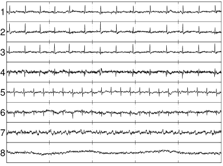
Figure 17: Estimated independent components using JADE.

The output of JADE for these data, i.e. the supposedly least dependent components, are shown in Fig. 17. Obviously channels 1-3 are dominated by the heartbeat of the mother, and channel 5 by that of the child. Channels 4 and 6 still contain large heartbeat components (of mother and child, respectively), but look much more noisy. Channels 7-8 seem to be dominated by noise, but with rather different spectral composition. The pairwise MIs of these channels are shown in Fig. 18 (left panel)footnote . One sees that most MIs are indeed small, but the first 3 components are still highly interdependent. This could be a failure of JADE, or it could mean that the basic model does not apply to these components. To decide between these possibilities, we minimized $I(X_{1}\ldots X_{8})$ by means of Eqs.(39) - (41). For each pair $(i,j)$ with $i,j=1\ldots 8$ we found the angle which minimized $I(X_{i}^{\prime},X_{j}^{\prime})-I(X_{i},X_{j})$, and repeated this altogether $\approx 10$ times. We did this both for $I^{(1)}$ and $I^{(2)}$, with $k=1$. We checked that $I(X_{1}\ldots X_{8})$, calculated directly, indeed decreased (from $I^{(1)}_{JADE}=1.782$ to $I^{(1)}_{\rm min}=1.160$, and from $I^{(2)}_{JADE}=2.264$ to $I^{(2)}_{\rm min}=1.620$).

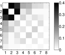
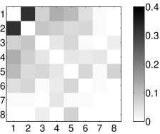
Figure 18: Left panel: Pairwise MIs between all ICA-components obtained by JADE, estimated with $I^{(1)},k=1$. The diagonal is set to zero.
Right panel: Pairwise MIs between the optimized channels shown in Fig. 19.

The resulting components are shown in Fig. 19. The first 2 components look now much cleaner, all the noise from the first 3 channels seems now concentrated in channel 3. But otherwise things have not changed very much. The pairwise MI after minimization are shown in Fig. 18 (right panel). As suggested by Fig. 19, channel 3 is now much less dependent on channels 1 and 2. But the latter are still very strongly interdependent, and a linear superposition of independent sources as in Eq.(37) can be ruled out. This was indeed to be expected: In any oscillating system there must be at least 2 mutually dependent components involved, and generically one expects both to be coupled to the output signal.

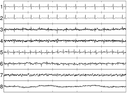
Figure 19: Estimated independent components after minimizing $I^{1}$.

To test for the uniqueness of the decomposition, we computed the variances

$$\sigma_{ij}={1\over 2\pi}\int_{0}^{2\pi}d\phi\left[I({\bf R}(\phi)(X_{i},X_{j}))-\overline{I(X_{i},X_{j})}\right]^{2}\;,$$ (42)

where

$$\overline{I(X_{i},X_{j})}={1\over 2\pi}\int_{0}^{2\pi}d\phi I({\bf R}(\phi)(X_{i},X_{j}))\;.$$ (43)

If $\sigma_{ij}$ is large, the minimum of the MI with respect to rotations is deep and the separation is unique and robust. If it is small, however, BSS can not be achieved since the decomposition into independent components is not robust. Results for the JADE output are shown in Fig. 20 (left panel), those for the optimized decomposition in the right panel of Fig. 20. The most obvious difference between them is that the first two channels have become much more clearly distinct and separable from the rest, while channel 3 is less separable from the rest (except from channel 5). This makes sense, since channels 3, 4, 7, and 8 now contain mostly Gaussian noise which is featureless and thus rotation invariant after whitening. Most of the signals are now contained in channels 5 (fetus) and in channels 1 and 2 (mother).

These results are in good agreement with those of Meinecke02 , but are obtained with less numerical effort and can be interpreted more straightforwardly.

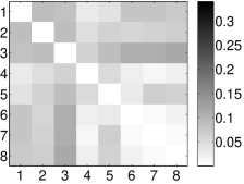
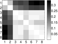
Figure 20: Square roots of variances, $\sqrt{\sigma_{ij}}$, of $I^{(1)}((X_{i},X_{j}))$ (with $k=1$) from JADE output (left panel) and after minimization of MI (right panel). Again, elements on the diagonal have been put to zero.

V Conclusion

We have presented two closely related families of mutual entropy estimators. In general they perform very similarly, as far as CPU times, statistical errors, and systematic errors are concerned. Their biggest advantage seems to be in vastly reduced systematic errors, when compared to previous estimators. This allows us to use them on very small data sets (even less than 30 points gave good results). It also allows us to use them in independent component analyses to estimate absolute values of mutual dependencies. Traditionally, contrast functions have been used in ICA which allow to minimize MI, but not to estimate its absolute value. We expect that our estimators will also become useful in other fields of time series and pattern analysis. One large class of problems is interdependencies in physiological time series, such as breathing and heart beat, or in the output of different EEG channels. The latter is particularly relevant for diseases characterized by abnormal synchronization, like epilepsy or Parkinson’s disease. In the past, various measures of interdependence have been used, including MI. But the latter was not employed extensively (see, however, pompe ), mainly because of the supposed difficulty in estimating it reliably. We hope that the present estimators might change this situation.

Acknowledgment:
One of us (P.G.) wants to thank Georges Darbellay for extensive and very fruitful e-mail discussions. We also want to thank Ralph Andrzejak, Thomas Kreuz, and Walter Nadler for numerous fruitful discussions, and for critically reading the manuscript.

Appendix

We collect here some well known facts about MI, in particular for higher dimensions, and some immediate consequences. The first important property of $I(X,Y)$ is its independence with respect to reparametizations. If $X^{\prime}=F(X)$ and $Y^{\prime}=G(Y)$ are homeomorphisms (smooth and uniquely invertible maps), and $J_{X}=||\partial X/\partial X^{\prime}||$ and $J_{Y}=||\partial Y/\partial Y^{\prime}||$ are the Jacobi determinants, then

$$\mu^{\prime}(x^{\prime},y^{\prime})=J_{X}(x^{\prime})J_{Y}(y^{\prime})\mu(x,y)$$ (44)

and similarly for the marginal densities, which gives

$$I(X^{\prime},Y^{\prime}) = \int\!\!\!\int dx^{\prime}dy^{\prime}\mu^{\prime}(x^{\prime},y^{\prime})\log{\mu^{\prime}(x^{\prime},y^{\prime})\over\mu^{\prime}_{x}(x^{\prime})\mu^{\prime}_{y}(y^{\prime})}$$ (45)

$$= \int\!\!\!\int dxdy\;\mu(x,y)\;\log{\mu(x,y)\over\mu_{x}(x)\mu_{y}(y)}$$

$$= I(X,Y)\;.$$

The next important property, checked also directly from the definitions, is

$$I(X,Y,Z)=I((X,Y),Z)+I(X,Y)\;.$$ (46)

This is analogous to the additivity axiom for Shannon entropies cover-thomas , and says that MI can be decomposed into hierarchical levels. By iterating it, one can decompose $I(X_{1}\ldots X_{n})$ for any $n>2$ and for any partitioning of the set $(X_{1}\ldots X_{n})$ into the MI between elements within one cluster and MI between clusters.

Let us now consider a homeomorphism $(X^{\prime},Y^{\prime})=F(X,Y)$. By combining Eqs.(45) and (46) we obtain

$$I(X^{\prime},Y^{\prime},Z) = I((X^{\prime},Y^{\prime}),Z)+I(X^{\prime},Y^{\prime})$$

$$= I((X,Y),Z)+I(X^{\prime},Y^{\prime})$$

$$= I(X,Y,Z)+[I(X^{\prime},Y^{\prime})-I(X,Y)]\;.$$

Thus, changes of high dimensional redundancies under reparametrization of some subspace can be obtained by calculating MIs in this subspace only. Although this is a simple consequence of well known facts about MI, it seems to have not been noticed before. It is numerically extremely useful, and would not hold in general for other interdependence measures. Again it generalizes to any dimension and to any number of random variables.

It is well known that Gaussian distributions maximize the Shannon entropy for given first and second moments. This implies that the Shannon entropy of any distribution is bounded from above by $(1/2)\log\det{\bf C}$ where ${\bf C}$ is the covariance matrix. For MI one can prove a similar result: For any multivariate distribution with joint covariance matrix ${\bf C}$ and variances $\sigma_{i}=C_{ii}$ for the individual (scalar) random variables $X_{i}$, the redundancy is bounded from below,

$$I(X_{1},\ldots X_{m})\geq{1\over 2}\log{\det{\bf C}\over\sigma_{1}\ldots\sigma_{m}}\;.$$ (48)

The r.h.s. of this inequality is just the redundancy of the corresponding Gaussian, and to prove Eq.(48) it we must show that the distribution minimizing the MI is Gaussian.

In the following we sketch only the proof for the case of 2 variables $X$ and $Y$, the generalization to $m>2$ being straightforward. We also assume without loss of generality that $X$ and $Y$ have zero mean. To prove Eq.(48), we set up a minimization problem where the constraints (correct normalization and correct second moments; consistency relations $\mu_{x}(x)=\int dy\;\mu(x,y)$ and $\mu_{y}(y)=\int dx\;\mu(x,y)$) are taken into account by means of Lagrangian multipliers. The “Lagrangian equation” $\delta L/\delta\mu(x,y)=0$ leads then to

$$\mu(x,y)={1\over Z}\;\mu_{x}(x)\;\mu_{y}(y)\;e^{-ax^{2}-by^{2}-cxy}$$ (49)

where $Z,a,b,$ and $c$ are constants fixed by the constraints. Since the minimal MI decreases when the variances $\sigma_{x}=C_{xx}$ and $\sigma_{y}=C_{yy}$ increase with $C_{xy}$ fixed, the constants $a$ and $b$ are non-negative. Eq.(49) is obviously consistent with $\mu(x,y)$ being a Gaussian. To prove uniqueness, we integrate Eq.(49) over $y$ and put $x=-iz/c$, to obtain

$$Z\;e^{-az^{2}/c^{2}}=\int dy\;e^{izy}\;[\mu_{y}(y)e^{-by^{2}}]\;.$$ (50)

This shows that $e^{-by^{2}}\mu_{y}(y)$ is the Fourier transform of a Gaussian, and thus $\mu_{y}(y)$ is also Gaussian. The same holds of course true for $\mu_{x}(x)$, showing that the minimizing $\mu(x,y)$ must be Gaussian, QED.

Finally, we should mention some possibly confusing notations. First, MI is often also called transinformation or redundancy. Secondly, what we call higher order redundancies are called higher order MIs in the ICA literature. We did not follow that usage in order to avoid confusion with cumulant-type higher order MIs matsuda .

References

- (1) T.M. Cover and J.A. Thomas, Elements of Information Theory (Wiley, New York 1991).
- (2) A. Renyi, Probability Theory (North Holland, Amsterdam 1971).
- (3) S. Roberts and R. Everson (Eds.), Independent Component Analysis: Principles and Practice (Cambridge Univ. Press, Cambridge 2001).
- (4) A. Hyvärinen, J. Karhunen, and E. Oja, Independent Component Analysis (Wiley, New York 2001).
- (5) Y.-I. Moon, B. Rajagopalam, and U. Lall, Phys. Rev. E 52, 2318 (1995).
- (6) R. Steuer, J. Kurths, C.O. Daub, J. Weise, and J. Selbig, Bioinformatics 18 Suppl. 2, S231 (2002).
- (7) A.M. Fraser and H.L. Swinney, Phys. Rev. A 33, 1134 (1986).
- (8) G.A. Darbellay and I. Vajda, IEEE Trans. Inform. Th. 45, 1315 (1999).
- (9) P. Grassberger, Phys. Lett. 128 A, 369 (1988).
- (10) M.S. Roulston, Physica D 125, 285 (1999).
- (11) R.L. Dobrushin, Theory Prob. Appl. 3, 462 (1958).
- (12) O. Vasicek, J. Royal Statist. Soc. B 38, 54 (1976).
- (13) E.S. Dudewicz and E.C. van der Meulen, J. Amer. Statist. Assoc. 76, 967 (1981);
- (14) B. van Es, Scand. J. Statist. 19, 61 (1992).
- (15) N. Ebrahimi, K. Pflughoeft, and E.S. Soofi, Statistics & Prob. Lett. 20, 225 (1994).
- (16) J.C. Correa, Commun. Statist. - Theory Meth. 24, 2439 (1995).
- (17) A.B. Tsybakov and E.C. van der Meulen, Scand. J. Statist. 23, 75 (1996).
- (18) R. Wieczorkowski and P. Grzegorzewksi, Commun. Statist. - Simula. 28, 541 (1999).
- (19) L.F. Kozachenko and N.N. Leonenko, Probl. Inf. Transm. 23, 95 (1987).
- (20) P. Grassberger, Phys. Lett. 107 A, 101 (1985).
- (21) R.L. Somorjai, “Methods for Estimating the Intrinsic Dimensionality of High-Dimensional Point Sets”, in Dimensions and Entropies in Chaotic Systems, G. Mayer-Kress, Ed. (Springer, Berlin 1986).
- (22) J.D. Victor, Phys. Rev. E 66, 051903-1 (2002).
- (23) G.A. Darbellay and I. Vajda, IEEE Trans. Inform. Th. 46, 709 (2000).
- (24) W.H. Press et al., Numerical Recipes (Cambridge Univ. Press, New York 1993).
- (25) P. Grassberger, Phys. Lett. 148 A, 63 (1990).
-
(26)
R. Hegger, H. Kantz, and T. Schreiber, TISEAN: Nonlinear
Time Series Analysis Software Package (ULR: www.mpipks-dresden.mpg.de/
~tisean). - (27) G.A. Darbellay, Computational Statistics and Data Analysis 32, 1 (1999)
- (28) G.A. Darbellay and I. Vajda, Inst. of Information Theory and Automation, Technical report No. 1921 (1998); to be obtained from http://siprint.utia.cas.cz/darbellay/
- (29) G.A. Darbellay, 3rd IEEE European Workshop on Computer-intensive Methods in Control and Data Processing, Prague, 7-9 September, 1998, pp. 83.
- (30) T.R. Hughes et al., Cell 102, 109 (2000); see also www.rii.com/publications/2000/cell_hughes.htm.
- (31) B.W. Silverman, Density Estimation for Statistics and Data Analysis (Chapman and Hall, London 1986).
- (32) F. Meinecke, A. Ziehe, M. Kawanabe, and K.-R. M ller, IEEE Trans. Biomed. Eng. 49, 1514 (2002).
- (33) J.-F. Cardoso, “Multidimensional independent component analysis”, Proceedings of ICASSP ’98 (1998).
- (34) J.-F. Cardoso and A. Souloumiac, IEE Proceedings F 140, 362 (1993).
- (35) B.L.R. De Moor (ed), ”Daisy: Database for the identification of systems”, www.esat.kuleuven.ac.be/sista/daisy (1997).
- (36) A. Ziehe, and K.-R. M ller. “TDSEP - an efficient algorithm for blind separation using time structure”, in L. Niklasson et al., eds., Proceedings of the 8th Int’l. Conf. on Artificial Neural Networks, ICANN’98, page 675 (Berlin, 1998).
- (37) In Figs. 18 to 20 we used , since the time sequences were sufficiently long to give very small statistical errors. To find components as independent as possible, we should have used much larger , since this would reduce statistical errors at the cost of increased but anyhow very small systematic errors. We checked that basically the same results were obtained with up to 100.
- (38) B. Pompe, P. Blidh, D. Hoyer, and M. Eiselt, IEEE Engineering in Medicine and Biology 17, 32 (1998).
- (39) H. Matsuda, Phys. Rev. E 62, 3096 (2000).