Functional Renormalization Group at Large $N$ for Disordered Elastic Systems, and Relation to Replica Symmetry Breaking

Abstract

We study the replica field theory which describes the pinning of elastic manifolds of arbitrary internal dimension $d$ in a random potential, with the aim of bridging the gap between mean field and renormalization theory. The full effective action is computed exactly in the limit of large embedding space dimension $N$. The second cumulant of the renormalized disorder obeys a closed self-consistent equation. It is used to derive a Functional Renormalization Group (FRG) equation valid in any dimension $d$, which correctly matches the Balents Fisher result to first order in $\epsilon=4-d$. We analyze in detail the solutions of the large-$N$ FRG for both long-range and short-range disorder, at zero and finite temperature. We find consistent agreement with the results of Mezard Parisi (MP) from the Gaussian variational method (GVM) in the case where full replica symmetry breaking (RSB) holds there. We prove that the cusplike non-analyticity in the large $N$ FRG appears at a finite scale, corresponding to the instability of the replica symmetric solution of MP. We show that the FRG exactly reproduces, for any disorder correlator and with no need to invoke Parisi’s spontaneous RSB, the non-trivial result of the GVM for small overlap. A formula is found yielding the complete RSB solution for all overlaps. Since our saddle-point equations for the effective action contain both the MP equations and the FRG, it can be used to describe the crossover from FRG to RSB. A qualitative analysis of this crossover is given, as well as a comparison with previous attempts to relate FRG to GVM. Finally, we discuss applications to other problems and new perspectives.

I Introduction

Elastic objects pinned by a quenched random potential are a relevant model for many experimental systems. It describes interfaces in magnets NattermannBookYoung ; LemerleFerreChappertMathetGiamarchiLeDoussal1998 which experience either short-range disorder (random bond), or long range (random field) disorder, the contact line of a liquid wetting a rough substrate PrevostRolleyGuthmann2002 ; ErtasKardar1994b , vortex lines in superconductors BlatterFeigelmanGeshkenbeinLarkinVinokur1994 ; GiamarchiLeDoussal1995 ; GiamarchiBookYoung ; NattermannScheidl2000 . It also provides powerful analogies, via mode coupling theory, to complex systems such as structural glasses BookYoung . One important observable is the roughness exponent $\zeta$ of the pinned manifold.

From the theoretical side, this problem still offers considerable challenges. It is the simplest example of a class of disordered systems, including random field magnets, where the so called dimensional reduction EfetovLarkin1977 ; AharonyImryShangkeng1976 ; Grinstein1976 ; ParisiSourlas1979 ; Cardy1983 ; NattermannBookYoung renders conventional perturbation theory trivial and useless at zero temperature. The elastic object is usually parameterized by a $N$ component vector $\vec{u}(x)$ in the embedding space $\mathbb{R}^{N}$, and $x\in\mathbb{R}^{d}$ is the coordinate in the internal space. Apart from the case of the directed polymer (DP) in $1+1$ dimensions ($d=1$, $N=1$), where some exact results were obtained Kardar1987 ; BrunetDerrida2000 ; BrunetDerrida2000a ; Johansson1999 ; PraehoferSpohn2000 , analytical results are scarce. One important challenge is to understand the DP for any $N$, due to its exact relation to the Kardar-Parisi-Zhang growth equation whose upper critical dimension is at present not known, and even its very existence is debated Laessig1995 ; Wiese1998a ; LassigKinzelbach1997 ; MarinariPagnaniParisi2000 .

Two main analytical approaches have been devised so far. Each succeeds in evading dimensional reduction, providing an interesting physical picture, but comes with its limitations. The first one is the mean field theory, the replica gaussian variational method (GVM) MezardParisi1991 in the statics and the off equilibrium dynamical version CugliandoloKurchanLeDoussal1996a ; CugliandoloLeDoussal1996b . The GVM approximates the replica measure by a replica symmetry broken (RSB) gaussian, equivalently, the Gibbs measure for $u$ as a random superposition of gaussians MezardParisi1991 , and is argued to be exact for $N=\infty$. It yields Flory values for the exponent $\zeta$. As for spin glasses, computing the next order corrections (i.e. in $1/N$) at the RSB saddle point is very arduous CarlucciDeDominicisTemesvari1996 ; DeDominicisEtAlBookYoung ; Goldschmidt1993 . One may question whether it is the most promising route, since it is as yet unclear whether the huge degeneracy of states encoded in the Parisi RSB is relevant to describe finite $N$. There seems to be some agreement that this type of RSB does not occur for low $d$ and $N$. Certainly, in the simpler but still-non trivial $d=0$ limit, Parisi type RSB found in the GVM should exist only at $N=\infty$, apart from the interesting so-called marginal case of logarithmic correlations CarpentierLeDoussal2001 . For the DP, another exactly solvable mean field limit is the Cayley tree and there too it is not clear how to meaningfully expand around that limit DerridaSpohn1988 ; CookDerrida1989 ; CookDerrida1989a .

The second main analytical method is the functional renormalization group (FRG) which performs a dimensional expansion around $d=4$ and was originally developped only to one loop, within a Wilson scheme Fisher1985b ; DSFisher1986 ; BalentsDSFisher1993 ; GiamarchiLeDoussal1995 . Its aim is to include fluctuations, neglected in the mean-field approaches. There too, the dynamics NattermanStepanowTangLeschhorn1992 ; LeschhornNattermannStepanow1996 ; NarayanDSFisher1992a ; NarayanDSFisher1992b ; ChauveGiamarchiLeDoussal2000 has been investigated. The FRG follows the second cumulant of the random potential $R(u)$ under coarse graining, a full function since the field is dimensionless in $d=4$. It was found that $R(u)$ becomes non-analytic already in the 1-loop equation at $T=0$ after a finite renormalization, at the Larkin scale.

Both methods circumvent dimensional reduction by providing a mechanism which is non-perturbative in the bare disorder. The GVM evades DR thanks to the RSB saddle point. The FRG escapes via the generation of a cusp-like non-analyticity in $R^{\prime\prime}(u)$ at $u=0$. Indeed, while the bare disorder correlator is an analytic function, FRG fixed points for the renormalized $R(u)$, perturbative in $\epsilon=4-d$, are found only in the space of non-analytic functions, and subject to the condition that the resulting exponent $\zeta$ is non-trivial. Both methods are disconcertingly different in spirit and it is an outstanding question in the theory of disordered systems how to compare and reconcile them. Comparisons were made between some predictions of the 1-loop FRG and of the GVM BalentsDSFisher1993 ; GiamarchiLeDoussal1995 . Balents and Fisher obtained the 1-loop FRG equation for any $N$ restricted to $O(\epsilon)$, and found that its solution reproduces the Flory value of $\zeta$ for LR disorder, but yields subtle corrections for SR disorder, exponential in $N$.

Physically both methods capture the metastable states beyond the Larkin scale $L_{c}$ and it is tempting to compare how they describe them. In BalentsBouchaudMezard1996 a coarse grained random potential was defined and it was found within the GVM that its correlator mimics the one in the FRG, exhibiting some non-analyticity which was interpreted in terms of shock-like singularities in the coarse grained disorder. Unfortunately, this analogy was demonstrated only around the Larkin scale, while a quantitative and more general connection able to reach perturbatively the true large scale behaviour, as is achieved in the field theoretic FRG, is still missing.

The need for a study of the FRG at large $N$ is all the more pressing since we have developped systematic higher loop approaches within the $\epsilon$-expansion ChauveLeDoussalWiese2000a ; LeDoussalWieseChauve2002 ; ChauveLeDoussal2001 . Within these studies, we have found that higher loop FRG equations for $R(u)$ at $u\neq 0$ contain non-trivial, potentially ambiguous “anomalous terms” involving the non-analytic structure of $R(u)$ at $u=0$. We have proposed a solution to lift these ambiguities in the statics at two loops ChauveLeDoussalWiese2000a ; LeDoussalWieseChauve2002 ; ChauveLeDoussal2001 . Since the large-$N$ limit allows in principle to handle higher-loop corrections (i.e. to treat any $\epsilon$) it should be useful to understand the many-loop structure of the field theory. Stated differently, we want to understand which physical quantity precisely does the FRG computes? Finally, developping a systematic $1/N$ expansion within the FRG for any $d$ should provide a novel handle to attack problems such as KPZ, maybe avoiding the need for spontaneous RSB altogether if it proves to be non-essential.

The aim of this paper is to study the FRG at large $N$. For this purpose we first perform an exact calculation of the effective action $\Gamma[u]$ of the replicated field theory at large $N$. Its value for a uniform mode and further expansion in cumulants yields a definition of the renormalized disorder consistent with field theoretic approaches. The second disorder cumulant is found to obey a closed self-consistent equation. All higher cumulants can be constructed recursively from the lower ones. It can be easily inverted below the Larkin scale and there the solution is analytic and corresponds to the replica symmetric solution of MP. Varying with respect to an infrared scale, here the mass, we obtain the FRG $\beta$-function in any $d$ at dominant order, $N=\infty$. The continuation beyond the Larkin scale is remarkably easier to perform on the resulting FRG equation. Its solution reveals that the FRG exactly reproduces the non-trivial result of the GVM with full RSB for small overlap. We also give a formula which yields the complete RSB solution for all overlaps. At no point in our derivation Parisi-RSB is invoked, as replica symmetry is broken explicitly here. Since our saddle point equations for the effective action contain both the MP equations and the FRG, it can be used to describe the crossover from FRG to RSB. A qualitative analysis of this crossover is given, as well as a comparison with previous attempts to relate the FRG to the GVM BalentsBouchaudMezard1996 . Finally, applications to other problems and new perspectives are discussed. A short version of this work has appeared in LeDoussalWiese2001 . In a related paper LeDoussalWiesePREPg , we give all details of the calculation of the $O(1/N)$ corrections, with the aim of understanding finite but large $N$.

The outline of the paper is as follows. In Section II we define the model, the effective action and its physical interpretation. In Section III we compute the effective action at large $N$, using the saddle point method and perform a cumulant expansion (Section IV). A graphical interpretation is given in Section V. In Section VI we establish the FRG equation at large $N$ (the $\beta$-function of the theory). Then in Section VII we perfom a detailed analysis of the FRG equation for a specific class of disorder correlators, both below and above the Larkin scale. In Section VIII we compare the FRG with the MP solution using RSB. First we recall the MP approach and find agreement with the predictions of the FRG calculation. Next we extend these results to an arbitrary disorder correlator for which the GVM gives full RSB. Finally we discuss the physical interpretation and compare our approach with the one of Ref. BalentsBouchaudMezard1996 . Section IX presents the conclusion. The appendices contain several generalizations, the calculation of the third and fourth disorder cumulant, finite temperature fixed points, and an analysis and comparison with the effective action in more conventional field theories.

II Model and program

II.1 Model and large-$N$ limit

We consider the general model for an elastic manifold of internal dimension $d$ embedded in a space of dimension $N$. The position of the manifold in the embedding space is described by a single valued displacement field $u(x)$, where $x$ belongs to the internal space and $u$ is a $N$ component vector which belongs to the embedding space. (Its components $u^{i}$, $i=1,\dotsc,N$, are specified below only when strictly necessary.) A well studied example is that of an interface (e.g. a domain wall in a magnet) where $d=2$ and $N=1$. There $u(x)$ denotes the height of the interface. Other examples are the directed polymer ($d=1$) in a $N$ dimensional space, which can be mapped to the $N$-dimensional Burgers and Kardar-Parisi- Zhang (KPZ) equations KPZ , or a vortex lattice in the absence of dislocations described by $d=3$, $N=2$, where $u(x)$ is there the deformation from the ideal crystal BlatterFeigelmanGeshkenbeinLarkinVinokur1994 ; GiamarchiLeDoussal1995 .

We will study here the equilibrium statistical mechanics of such an elastic manifold in presence of quenched disorder, modeled by a random potential $V(x,u(x))$. It is described, in a given realization of the random potential, by the partition function

$${\cal Z}_{V}=\int{\cal D}[u]\,{\mathrm{e}}^{-{\cal H}_{V}[u]/T}\ ,$$ (2.1)

where

$$\frac{{\cal H}_{V}[u]}{T}=\int_{q}~{}\frac{1}{2}~{}C(q)^{-1}~{}u(-q)\cdot u(q)+\frac{1}{T}\int_{x}V(x,u(x))$$ (2.2)

consists out of an elastic energy (expressed here in Fourier space and taken to be isotropic), and of a pinning energy due to disorder. Here and below we denote

$$\int_{q}:=\int\frac{{\mathrm{d}}^{d}q}{(2\pi)^{d}}\quad,\quad\int_{x}:=\int{\mathrm{d}}^{d}x$$ (2.3)

and $u\cdot v=\sum_{i=1}^{N}u^{i}v^{i}$. Throughout, square brackets as e.g. in $A[u]$ denote a functional, here $A$ of the field $u_{a}(x)$, while parenthesis as in $A(u)$ denote functions.

A convenient form for the inverse bare propagator, used below, is:

$$C(q)^{-1}=\frac{q^{2}+m^{2}}{T}\ ,$$ (2.4)

where $T$ is the temperature and the elastic constant is set to unity by a choice of units. The role of the additional mass term $m$ will be discussed below. An additional small scale (ultraviolet, UV) cutoff $\Lambda$ is implied here and will be made explicit when needed.

This model is highly non-trivial and, apart from the cases of $N=1$ and $d=0,1$, very few exact results are known Kardar1987 ; BrunetDerrida2000 ; BrunetDerrida2000a ; Johansson1999 ; PraehoferSpohn2000 ; LeDoussalMonthus2003 . To obtain exact results for large embedding space $N\to\infty$, we need to consider a fully isotropic version of the model with $O(N)$ symmetry such that the model remains non-trivial in that limit. As in standard large-$N$ treatment (as for instance of the $\phi^{4}$ $O(N)$ model) one defines the rescaled field

$$v(x)=\frac{u(x)}{\sqrt{N}}\ .$$ (2.5)

We will freely switch from one to the other in the following. One also chooses the distribution of the random potential to be $O(N)$ rotationally invariant. It can be parameterized by its set of connected cumulants, of the form

$$\overline{V(x,u)V(x^{\prime},u^{\prime})}=R(|u-u^{\prime}|)\delta^{d}(x-x^{\prime})$$

$$\qquad=NB((v-v^{\prime})^{2})\delta^{d}(x-x^{\prime})\qquad$$ (2.6)

$$\overline{V(x_{1},u_{1})\dots V(x_{p},u_{p})}^{\mathrm{con}}$$

$$\qquad=N\delta_{x_{1},\dots,x_{p}}(-1)^{p}S^{(p)}(v_{1},\dots,v_{p})\ ,\quad p\geq 3~{}~{}~{}$$ (2.7)

$$\delta_{x_{1},\dotsc,x_{p}}:=\prod_{i=2}^{p}\delta^{d}(x_{1}-x_{i})$$ (2.8)

This adequately models the case of uncorrelated (or short-range correlated) disorder in the internal space, studied here. The second cumulant, which plays the central role, is thus defined in terms of a function $B(z)$. The higher cumulants are not strictly necessary in the bare model, but they appear, as we will see, under coarse graining. The distribution of disorder being translationally invariant, these functions satisfy $S^{(p)}(v_{1}+v,\dots,v_{p}+v)=S^{(p)}(v_{1},\dots,v_{p})$ for any $v$. The model studied here is thus a slight generalization of the model studied by Mezard and Parisi MezardParisi1991 , henceforth also referred to as MP, in the same limit.

Although we will consider the general case, it is useful, as in MP MezardParisi1991 to define two sets of simple models for which more specific results will be given. These are, respectively, the gaussian, short-range (SR) disorder, correlator

$$B(z)=ge^{-z}$$ (2.9)

and the power-law correlations

$$B(z)=\frac{g}{(\gamma-1)}(a^{2}+z)^{1-\gamma}\ ,$$ (2.10)

which, for infinite $N$ always corresponds to long-range (LR) disorder, a different universality class, as we will see below. For finite $N$, the long-range disorder corresponds, at the bare level, to $\gamma<1+N/2$; but this is modified at the renormalized level, and the true frontier LR-SR for finite $N$ is non-trivial.

II.2 Program

Having defined the model, and before turning to calculations, let us first outline what we aim at. All the considerations in the present section are valid for any $N$, but, since in the next section we will consider the large $N$ limit explicitly, we already make apparent the rescalings.

The model defined above has already been studied in MP MezardParisi1991 . One of the aims of this study was to compute the roughness exponent of the manifold, defined from the 2-point function as

$$\overline{\left<(u(x)-u(x^{\prime}))^{2}\right>}\sim A|x-x^{\prime}|^{2\zeta}\ .$$ (2.11)

Besides the roughness exponent $\zeta$, the amplitude $A$ is also of interest whenever it is universal, as it is the case e.g. for long range disorder. To this aim the model was replicated ($u\to u_{a}$), averaged over disorder and self-consistent saddle point equations where derived for the 2-point function

$$G_{ab}(q)\equiv\left<v_{a}(q)v_{b}(-q)\right>\ .$$ (2.12)

This can always be done in a large-$N$ limit, and is then solved via a RSB ansatz.

Our goal is in a sense broader. We want to understand the full structure of the field theory, i.e. all correlation functions and not only the 2-point one. We will thus instead study the generating function of correlations as well as the effective action functional which yields the renormalized vertices. This program, defined here, will be carried out in the following sections explicitly for large $N$. In this article we will restrict ourselves to dominant order, but the aim is to understand large but finite $N$, including calculating of $1/N$ corrections. This is deferred to LeDoussalWiesePREPg .

II.2.1 Effective action and field theory

All physical observables for any $N$ can be obtained from the replicated action in presence of a source, i.e. an external force $J_{a}(x)$ acting on each replica:

$${\cal Z}[J]=\overline{\int\prod_{a}{\cal D}[u_{a}]e^{-\sum_{a}H_{V}[u_{a}]/T+\int_{x}\sum_{a}J_{a}(x)\cdot u_{a}(x)}}\ ,$$ (2.13)

where $u_{a}(x)$, $a=1,\dots,n$ are the replicated fields (each one being an $N$ component vector $u^{i}_{a}(x)$). Differentiating with respect to the replicated source $J_{a}(x)$ in the limit $n\to 0$ yields all correlation functions. The finite-$n$ information is also interesting. For instance from

$${\cal Z}:={\cal Z}[J=0]=\overline{\exp(-n{\cal F}_{V}/T)}$$ (2.14)

one can retrieve the sample to sample distribution of the free energy ${\cal F}_{V}=-T\ln{\cal Z}_{V}$, as was done e.g. in a finite size system for $d=1$ BrunetDerrida2000a ; GorokhovBlatter1999 . Thus, unless specified we will keep $n$ arbitrary.

One can explicitly perform the disorder average in (2.13):

$${\cal Z}[J] = \int\prod_{a}{\cal D}[u_{a}]{\mathrm{e}}^{-N{\cal S}[u,j]}$$ (2.15)

$${\cal S}[u,j] = \frac{1}{2}\int_{q}C(q)^{-1}v_{a}(-q)\cdot v_{a}(q)$$ (2.16)

$$+\int_{x}[U(\chi(x))-j_{a}(x)\cdot v_{a}(x)]\qquad\ ,$$

where here $\chi_{ab}(x)=v_{a}(x)\cdot v_{b}(x)$ and here and below summations over repeated replica indices are implicit. We have rescaled the source in a manner complementary to the field:

$$J_{a}(x)=\sqrt{N}j_{a}(x)\ .$$ (2.17)

We have also introduced the bare interaction potential

$$U(\chi)=\frac{-1}{2T^{2}}\sum_{ab}B(\tilde{\chi}_{ab})-\frac{1}{3!T^{3}}\sum_{abc}S(\tilde{\chi}_{ab},\tilde{\chi}_{bc},\tilde{\chi}_{ca})+\dots\ ,$$ (2.18)

which is a function of a $n$ by $n$ replica matrix $\chi_{ab}$ and has a cumulant expansion in terms of sums with higher numbers of replicas. Because of translational symmetry and $O(N)$ invariance it depends only on the matrix

$$\tilde{\chi}_{ab}:=\chi_{aa}+\chi_{bb}-\chi_{ab}-\chi_{ba}$$ (2.19)

and the form of each cumulant is restricted. For instance one has $S^{(3)}(v_{1},v_{2},v_{3})=S((v_{1}-v_{2})^{2},(v_{2}-v_{3})^{2},(v_{3}-v_{1})^{2})$ etc.. The matrix potential $U(\chi)$ can thus be considered as a convenient way to parameterize the disorder (here the bare disorder).

The physical object which contains the information about the field theory at large scale is the effective action. It is the generating function of the 1-particle irreducible diagrams and in conventional field theories its formal expansion in powers of the field yields the renormalized vertices. All correlation functions are then obtained simply as tree diagrams from these renormalized vertices. In particular it is known that within a $d=4-\epsilon$ expansion at zero temperature to at least 2-loop order the theory can be renormalized (i.e. rendered UV finite and yielding universal results) by considering counter-terms only to the second cumulant. The latter is a function $R(u)$, and can be viewed as the set of all coupling constants which simultaneously become marginal in $d=4$. To probe renormalizability to any number of loops, we want to compute the effective action from first principles.

The effective action functional is defined as a Legendre transform:

$$\Gamma[u]+{\cal W}[J] = \int_{x}\sum_{a}J_{a}(x)\cdot u_{a}(x)$$ (2.20)

$${\cal W}[J] = \ln{\cal Z}[J]\ .$$ (2.21)

Strictly speaking the definition is the convex envelope $\Gamma[u]=\min_{J}(\int_{x}\sum_{a}J_{a}(x)\cdot u_{a}(x)-{\cal W}[J])$. Here we apply the definition to the replicated action, and will content ourselves with the differential definition

$$\frac{\delta\Gamma[u]}{\delta u_{a}(x)} = J_{a}(x)$$ (2.22)

$$\frac{\delta{\cal W}[J]}{\delta J_{a}(x)} = u_{a}(x)\ ,$$ (2.23)

which relates a pair of values $(J,u)$, later also denoted by $(J[u],u)$. Since $\Gamma[u]$ defines the renormalized vertices, its zero momentum limit defines the renormalized disorder. Thus in order to compute the renormalized disorder, we only need to compute $\Gamma[u]$ (per unit volume) for a uniform configuration of the replica field $u_{a}(x)=u_{a}=\sqrt{N}v_{a}$ (a so-called fixed background configuration). Because of the statistical tilt symmetry SchulzVillainBrezinOrland1988 ; HwaFisher1994b ; stsproof , i.e. invariance of disorder term in the replicated action (2.16) under the translation $v_{a}(x)\to v_{a}(x)+w(x)$, and of the $O(N)$ invariance one can argue, and this is what we find below, that for the model (2.4) the scaled effective action per unit volume (which for a uniform mode is simply a function of $u_{a}$) should have the following form

$$\hat{\Gamma}(v):=\frac{1}{L^{d}N}\Gamma(u)=\frac{1}{2T}m^{2}v_{a}^{2}+\tilde{U}(vv)\ ,$$ (2.24)

where $L^{d}$ is the volume of the system, and here and below we use the notation:

$$vv:=v_{a}\cdot v_{b}$$ (2.25)

for the $n$ by $n$ replica matrix. This defines the renormalized disorder. Furthermore, whenever $\tilde{U}(vv)$ can be expanded, up to a constant, in the form:

$$\tilde{U}(vv)=\frac{-1}{2T^{2}}\sum_{ab}\tilde{B}(v_{ab}^{2})-\frac{1}{3!T^{3}}\sum_{abc}\tilde{S}(v_{ab}^{2},v_{bc}^{2},v_{ca}^{2})+\dots\ ,$$ (2.26)

where here and in the following we denote

$$v_{ab}:=v_{a}-v_{b}\ ,$$ (2.27)

then (2.26) defines the renormalized cumulant functions $\tilde{B}(z)$ etc.. As we will see below this is correct up to some very subtle behavior at coinciding replica vectors (i.e. $v_{ab}=0$ for some pair $a,b$). Also note that the constant part $\tilde{U}(v.v=0)$ is the free energy.

The main result of the following sections will be the exact calculation of the uniform part of the effective action, i.e. of the function $\tilde{U}(vv)$. This will be performed within a large $N$ expansion:

$$\tilde{U}(vv)=\tilde{U}_{0}(vv)+\frac{1}{N}\tilde{U}_{1}(vv)+\dotsb$$ (2.28)

and here we will obtain the dominant order $\tilde{U}_{0}(vv)$; the corrections $\tilde{U}_{1}(vv)$ are calculated in LeDoussalWiesePREPg . It will be a function of a scale parameter. We choose to add a mass-term $m$ which provides such a scale. It is a convenient choice since for $m=\infty$ one has $\tilde{U}=U$: Fluctuations are totally suppressed and the effective action equals the action. One can then progressively lower the mass down to zero, starting from this initial condition, since ultimately one is interested in the massless limit. Another choice is to change the UV cutoff, as will be discussed again below.

It is now useful to give a more direct physical interpretation of this quantity, in addition to the above field theoretic interpretation.

II.2.2 Effective action as the distribution of the order parameter

The effective action for a uniform background is also known to be related to the distribution of the order parameter. Let us recall the relation for a simple pure ferromagnet. The unnormalized probability distribution of the order parameter $\Phi=\frac{1}{L^{d}}\int_{x}\phi(x)$ where $\phi(x)$ is the local magnetization is by definition

$$Z(\Phi)=\int{\cal D}[\phi]\,\delta\left(\Phi-\frac{1}{L^{d}}\int_{x}\phi(x)\right){\mathrm{e}}^{-S[\phi]}\ ,$$ (2.29)

where $S[\phi]$ is the action which describes the ferromagnet (e.g. a $\phi^{4}$ theory or a Landau Ginsburg model). The functional $W(J)$ evaluated for a uniform $J$ reads:

$$W(J) = \int{\mathrm{d}}\Phi\,Z(\Phi)\,{\mathrm{e}}^{L^{d}J\Phi}$$ (2.30)

$$= \int{\mathrm{d}}\Phi\,{\mathrm{e}}^{L^{d}(\frac{1}{L^{d}}\ln Z(\Phi)+J\Phi)}\ .$$

In the large-volume limit, the saddle point can be taken and since the Legendre transform is involutive, this yields the relation between the effective action at $q=0$ per unit volume and the probability distribution of the order parameter as:

$$-\hat{\Gamma}(\Phi)=\lim_{L\to\infty}\frac{1}{L^{d}}\ln Z(\Phi)\ .$$ (2.31)

In the thermodynamic limit the effective action per unit volume can very well be a non-analytic function. This is the case e.g. in the ferromagnetic phase where its left and right second derivatives at $\Phi=M$ do not coincide ($M$ is the spontaneous magnetization per unit volume). While the right derivative at $\Phi=M$ is related to the inverse susceptibility, the left one is zero, mathematically due to the prescription to take the convex envelope, and physically because one can always lower the magnetization at no cost in free energy per unit volume by introducing a domain wall. The above property (2.31) can be extended to a given $q$ mode. Finally, note that in $d=0$ the above does not hold since there is no large factor $L^{d}$, and the probability distribution is directly given by the action $S(\Phi=\phi)$.

What is then the physical meaning of the quantity that we will be computing in the next sections? Let us in analogy to the magnetization for a ferromagnet define the center of mass of an interface:

$$w=\frac{1}{N^{1/2}L^{d}}\int_{x}u(x)\ .$$ (2.32)

Since we have added a mass in the elastic energy (2.4), which acts as an extra quadratic well bounding the fluctuations of the interface, the disorder-induced fluctuations of the center of mass are always finite. One expects that they diverge typically as $w\sim m^{-\zeta}$ as $m\to 0$, thus their behavior as a function of $m$ is of high interest and yields e.g. the information about the roughness exponent.

One can then define the probability distribution $P_{V}(w)$ of the center of mass of the interface in a given realization of the random potential $V$ (and in presence of the quadratic well induced by the mass). One can see that by definition the generating function for a uniform $j$ is the Laplace transform of the probability distribution of $w$, namely

$$Z(j)=\int{\mathrm{d}}w_{1}\ldots{\mathrm{d}}w_{n}\overline{P_{V}(w_{1})\dots P_{V}(w_{n})}\,{\mathrm{e}}^{-NL^{d}\sum_{a}j_{a}w_{a}}\ ,$$ (2.33)

then by the same saddle point argument as for the ferromagnet one expects, at least naively, that

$$\hat{\Gamma}[\{w_{a}\}]=-\lim_{L\to\infty}\frac{1}{NL^{d}}\ln\overline{P_{V}(w_{1})\dots P_{V}(w_{n})}\ .$$ (2.34)

Symbolically one can write:

$$\overline{P_{V}(w_{1})\dots P_{V}(w_{n})}\approx e^{-L^{d}N\hat{\Gamma}[\{w_{a}\}]}\ ,$$ (2.35)

provided this is taken with a grain of salt. Thus one can also think of the renormalized disorder $N\tilde{U}(v\cdot v)$ as parameterizing the set of correlations of an effective equivalent toy model ($d=0$) which has the same set of correlations as the center of mass variable in the original model.

The $p$-th connected moment of the center of mass is identical, up to a volume factor, to the zero momentum limit of the connected m point correlator of the $u$ field, e.g.

$$\left<w_{a_{1}}\dots w_{a_{p}}\right>_{c}=\frac{1}{L^{d}}\left<v_{a_{1}}(q_{1})\dots v_{a_{p}}(q_{p})\right>_{c}|_{q_{i}=0}$$ (2.36)

and, once the effective action is known, both can thus be obtained in principle as the sum of all tree graphs made from $\hat{\Gamma}[v]$ vertices. For instance the 2-point function should be obtainable from:

$$\left<w_{a}w_{b}\right>=\frac{1}{L^{d}}G_{ab}(q=0)=\frac{1}{L^{d}}[\hat{\Gamma}^{\prime\prime}[v=0]]^{-1}_{ab}$$ (2.37)

and the connected 4-point function from:

$$\left<w_{a}w_{b}w_{c}w_{d}\right>^{\mathrm{con}} = \frac{1}{L^{d}}G_{abcd}(q_{i}=0)$$ (2.38)

$$= \frac{1}{NL^{d}}\sum_{efgh}[\hat{\Gamma}^{\prime\prime}[v=0]]^{-1}_{ae}[\hat{\Gamma}^{\prime\prime}[v=0]]^{-1}_{bf}$$

$$\times[\hat{\Gamma}^{\prime\prime}[v=0]]^{-1}_{cg}[\hat{\Gamma}^{\prime\prime}[v=0]]^{-1}_{dh}$$

$$\times\hat{\Gamma}^{\prime\prime\prime\prime}[v=0]_{efgh}$$

this however assumes analyticity, which as we will see below, does not always hold. Another integral relation holds

$$\left<w_{a}w_{b}\right> \equiv \int{\mathrm{d}}w_{1}\dotsb{\mathrm{d}}w_{n}\,w_{1}w_{2}\overline{P_{V}(w_{1})\dots P_{V}(w_{n})}$$ (2.39)

$$\equiv W^{\prime\prime}_{12}(j=0)$$

$$\approx \int{\mathrm{d}}w_{1}\dotsb{\mathrm{d}}w_{n}\,w_{1}w_{2}e^{-L^{d}N\tilde{\Gamma}[\{w_{a}\}]}\ .$$

III Calculation of the effective action

Let us now consider explicitly the large $N$ limit. One can rewrite for any $N$ the starting generating function (2.15-2.16) as:

$${\cal Z}[J]=\int{\cal D}[u]{\cal D}[\chi]{\cal D}[\lambda]{\mathrm{e}}^{-N{\cal S}[u,\chi,\lambda,J]}$$ (3.1)

$${\cal S}[u,\chi,\lambda,j]=\frac{1}{2}\!\int_{q}C(q)^{-1}v_{a}(-q)\cdot v_{a}(q)-\!\int_{x}j_{a}(x)\cdot v_{a}(x)\qquad$$

$$+\int_{x}U(\chi(x))-\frac{1}{2}i\lambda_{ab}(x)\left[\chi_{ab}(x)-v_{a}(x)\cdot v_{b}(x)\right]\ ,$$ (3.2)

where the replica matrix field $\chi(x)\equiv\chi_{ab}(x)$ has been introduced through a Lagrange multiplier matrix $\lambda_{ab}(x)$. Here and below summations over repeated replica indices are implicit. One can then explicitly perform the functional integration over the field $u(x)$ and obtain:

$${\cal Z}[J] = \int D\chi D\lambda e^{-NS[\chi,\lambda,j]}$$ (3.3)

$$S[\chi,\lambda,j] = \frac{1}{2}{\mathrm{\bf Tr}}\ln(C^{-1}+i\lambda)$$ (3.4)

$$+\int_{x}U(\chi(x))-\frac{i}{2}\lambda^{ab}(x)\chi^{ab}(x)$$

$$-\frac{1}{2}\int_{x,x^{\prime}}j_{a}(x)(C^{-1}+i\lambda)^{-1}_{ax,bx^{\prime}}j_{b}(x^{\prime})\ ,\qquad$$

where the inversion and trace are performed in both replica space and spatial coordinate space.

It has now the standard form for a saddle point evaluation of the functional ${\cal W}(J)=\ln{\cal Z}(J)$ except that the saddle point is not, in general, uniform in space. It is useful to define the scaled functional $\tilde{W}(j)$ through

$${\cal W}[J]=N\tilde{W}[j=J/\sqrt{N}]\ ,$$ (3.5)

which has a well defined large-$N$ limit and can be expanded in $1/N$ as:

$$\tilde{W}[j]=W^{0}[j]+\frac{1}{N}W^{1}[j]+\dots\ .$$ (3.6)

Deferring the calculation of the corrections to a future publication LeDoussalWiesePREPg , we obtain here the dominant order in $1/N$ as:

$$W^{0}[j]=-S[\chi_{j},\lambda_{j},j]\ ,$$ (3.7)

where $\chi_{j}$ and $\lambda_{j}$ depend on $j(x)$ and are the solutions of the saddle point equations obtained respectively by setting to zero the functional derivatives (at fixed $j(x)$):

$$\frac{\delta S[\chi,\lambda,j]}{\delta\lambda_{ab}(x)}\bigg{|}_{\chi=\chi_{j},\lambda=\lambda_{j}} = 0$$ (3.8)

$$\frac{\delta S[\chi,\lambda,j]}{\delta\chi_{ab}(x)}\bigg{|}_{\chi=\chi_{j},\lambda=\lambda_{j}} = 0\ .$$ (3.9)

The result is

$$\chi_{j}^{ab}(x) = (G_{j})_{ax,bx}+(G_{j}:j)_{ax}\cdot(G_{j}:j)_{bx}\qquad$$ (3.10)

$$i\lambda_{j}^{ab}(x) = 2\partial_{ab}U(\chi_{j}(x))$$ (3.11)

$$G_{j}^{-1} = C^{-1}+i\lambda_{j}\ ,$$ (3.12)

where $G_{j}$ is a matrix with both replica indices and spatial coordinates and inversion is carried out for both. Here and below, replica indices are raised whenever explicit dependency is given, e.g. $\chi_{ab}\equiv\chi_{j}^{ab}$. The notation for the $N$-component vector $(G:j)^{i}_{bx}=\sum_{c}\int_{y}G_{bx,cy}j^{i}_{c}(y)$ is a shorthand for a matrix product, and everywhere we denote by

$$\partial_{ab}U(\phi):=\partial_{\phi_{ab}}U(\phi)$$ (3.13)

the simple derivative of the function $U(\phi)$ with respect to its matrix argument $\phi_{ab}$. Of course, if, for a given $j(x)$ there are several solutions to these equations, then one must sum over all saddle points, to the same order

$${\cal W}[j]\approx\ln\Big{(}\sum_{\mathrm{sp}}{\mathrm{e}}^{-NS[\chi_{\mathrm{sp}}(j),\lambda_{\mathrm{sp}}(j),j]}\Big{)}\ .$$ (3.14)

This case will be discussed below, for now we ignore this possible complication, as well as issues of stability of the saddle point.

Now we want to take the Legendre transform and trade the variable $j$ for the variable $v$ to obtain the effective action $\Gamma[u]$. One also defines the scaled functional, and its $1/N$ expansion through:

$$\Gamma[u] = N\tilde{\Gamma}[v=u/\sqrt{N}]$$ (3.15)

$$\tilde{\Gamma}[v] = \Gamma_{0}[v]+\frac{1}{N}\Gamma_{1}[v]+\dots\ .$$ (3.16)

Then ($\tilde{\Gamma}[v]$,$\tilde{W}[j]$) and ($\tilde{\Gamma}_{0}[v]$,$W_{0}[j]$) are also two pairs of Legendre transforms. Thus the dominant order of the effective action functional in the large-$N$ limit is given by

$$\Gamma_{0}[v]=\int_{x}v_{a}(x)\cdot j^{a}_{v}(x)-W_{0}[j_{v}]$$ (3.17)

with $W_{0}[j]$ given by (3.7), (3.12) and where $j_{v}(x)$ is the $v(x)$-dependent source solution of:

$$\frac{\delta W_{0}[j_{v}]}{\delta j^{a}_{v}(x)}=v_{a}(x)\ .$$ (3.18)

One can now derive a self-consistent functional saddle point equation for $\Gamma_{0}[v]$. First we establish the relation between $v$ and $j_{v}$, namely

$$v_{a}(x)=(G_{v}:j_{v})_{ax}\quad\Leftrightarrow\quad j_{v}^{a}(x)=(G_{v}^{-1}:v)_{ax}\ ,$$ (3.19)

where from now on we define

$$G_{v}:=G_{j_{v}}\ .$$ (3.20)

Eq. (3.19) is obtained noting that

$$v_{a}(x) = \frac{\delta W_{0}[j_{v}]}{\delta j^{a}_{v}(x)}=-\frac{{\mathrm{d}}}{{\mathrm{d}}j_{a}(x)}S[\chi_{j},\lambda_{j},j]\bigg{|}_{j=j_{v}}$$

$$= -\int_{y}\left[\frac{\partial\chi_{j}(y)}{\partial j_{a}(x)}\frac{\partial S}{\partial\chi_{j}(y)}+\frac{\partial\lambda_{j}(y)}{\partial j_{a}(x)}\frac{\partial S}{\partial\lambda_{j}(y)}\right]\bigg{|}_{j=j_{v}}$$

$$-\frac{\partial S}{\partial j_{a}(x)}\bigg{|}_{j=j_{v}}=-\frac{\partial S}{\partial j_{a}(x)}\bigg{|}_{j=j_{v}}=(G_{j_{v}}:j_{v})_{ax}\ ,$$

where we have used the saddle-point equations (3.8), (3.9).

We can now use (3.19) in the saddle point equations (3.8), (3.9) and defining

$$\chi_{v}:=\chi_{j_{v}}\ ,\qquad\lambda_{v}:=\lambda_{j_{v}}\ ,$$

this yields a self-consistent equation for $\chi_{v}(x)$

$$\chi^{ab}_{v}(x) = v_{a}(x)\cdot v_{b}(x)+(G_{v})_{ax,bx}$$ (3.22)

$$(G_{v}^{-1})_{ax,by} = (C^{-1})_{x,y}\delta_{ab}+2\partial_{ab}U(\chi_{v}(x))\delta^{d}(x-y)\ ,$$

which is also a self-consistent equation for $G_{v}$. Since the Legendre transform is involutive, one can also write:

$$\frac{\delta\Gamma_{0}[v]}{\delta v_{a}(x)}=j_{a}(x)=(G_{v}^{-1}:v)_{ax}\ ,$$ (3.24)

which determines the derivative of $\Gamma_{0}[v]$ once (LABEL:scG) is solved.

One can however do better. Using (3.19) in (3.17) one obtains the effective action for a spatially varying field $v(x)$:

$$\Gamma_{0}[v]=v:(G_{v}^{-1}):v+S[\chi_{v},\lambda_{v},j_{v}]\ ,$$ (3.25)

which gives

$$\Gamma_{0}[v] = \frac{1}{2}\int_{xy}C^{-1}_{ax,by}v_{a}(x)v_{b}(y)$$

$$+\frac{1}{2}{\mathrm{\bf Tr}}\ln(C^{-1}+2\partial U(\chi_{v}))+\int_{x}U(\chi_{v}(x))$$

$${+}\!\int_{x}\!v_{a}(x)\partial_{ab}U(\chi_{v}(x))v_{b}(x){-}\chi^{ab}_{v}(x)\partial_{ab}U(\chi_{v}(x))\ .$$

It is interesting to rewrite it with the help of (LABEL:scG) as a functional of $G_{v}$ and $v$ only:

$$\Gamma_{0}[G_{v},v] := \Gamma_{0}[v]=-\frac{1}{2}{\mathrm{\bf Tr}}\ln G_{v}$$ (3.27)

$$+\frac{1}{2}\int_{xy}C^{-1}_{ax,by}\left[v_{a}(x)v_{b}(y)+(G_{v})_{ax,by}\right]$$

$$+\int_{x}U(vv(x)+(G_{v})_{x,x})\ .$$

We have dropped a constant $\sim n$. (3.27) has the property

$$\partial_{G}\Gamma_{0}[G,v]|_{G=G_{v}}=0\ ,$$ (3.28)

where the derivative acts only on $G$, leaving fixed all $v$, since this coincides with the saddle point equation (LABEL:scG). This makes apparent that it can also be obtained from a variational method where the average of the field is fixed, as we detail in Appendix A. Since the explicit non-trivial $v$-dependence in (3.27) using (LABEL:scG) is purely in terms of the bilinears $v_{a}(x)\cdot v_{b}(x)$ at the same space points, it also shows that one can write:

$$\Gamma_{0}[v]=\frac{1}{2}\,v:C^{-1}:v+\tilde{U}_{0}[v\cdot v]\ ,$$ (3.29)

where the interaction (i.e. disorder) part satisfies

$$\frac{\delta\tilde{U}_{0}[v\cdot v]}{\delta(v_{a}(x)\cdot v_{b}(y))}=0\ ,\qquad x\neq y$$ (3.30)

and is the solution of a self-consistent functional equation:

$$\!\!\!\frac{\delta\tilde{U}_{0}[v\cdot v]}{\delta(v_{a}(x)\cdot v_{b}(x))}=\partial_{ab}U(vv(x)+(G_{v})_{x,x})$$ (3.31)

$$\!\!\!(G_{v}^{-1})_{ax,by}=(C^{-1})_{x,y}\delta_{ab}+\frac{\delta\tilde{U}_{0}[v\cdot v]}{\delta(v_{a}(x)\cdot v_{b}(x))}\,\delta^{d}(x-y)\ .$$

A generalization of this equation is presented in Appendix B.

IV Self-consistent equation for the renormalized disorder

IV.1 Uniform configuration and saddle point equation

Let us now consider the simpler problem of computing the effective action for a uniform field configuration, which can be solved self-consistently. To be more specific we will focus on the form (2.4) for the elastic energy. Also, to simplify notations and since we will restrict ourselves to dominant order in $1/N$, we drop the index $0$, so we set:

$$\Gamma_{0}\to\tilde{\Gamma}\quad,\quad\tilde{U}_{0}\to\tilde{U}$$ (4.1)

and so on.

For a uniform field $v_{a}(x)=v_{a}$ the effective action (3.29) per unit volume takes the form:

$$\hat{\Gamma}(v):=\frac{1}{L^{d}}\tilde{\Gamma}(v)=\frac{1}{2T}m^{2}v_{a}^{2}+\tilde{U}(vv)\ .$$ (4.2)

Note that these are now simply functions (not functionals) of a $N\times n$-component vector, and $\tilde{U}(vv)$ is a function of the $n$ by $n$ matrix $v_{a}v_{b}$.

Eq. (3.27) yields also a formula for $\tilde{U}_{0}(vv)$ (up to a constant):

$$\tilde{U}(vv) = U(\chi_{v})+\frac{1}{2}\int_{q}\mbox{tr}\Big{\{}\ln\!\big{(}(q^{2}+m^{2})\delta+2T\partial U(\chi_{v})\big{)}$$ (4.3)

$$+(q^{2}+m^{2})\left[(q^{2}+m^{2})\delta+2T\partial U(\chi_{v})\right]^{-1}\Big{\}}\ .\qquad$$

The trace acts in replica space, and the log is a function of a matrix, to be defined as usual. Since (4.3) contains the derivative $\partial_{ab}\tilde{U}^{0}(vv)$ we must first determine the latter. One finds that analogous to (3.31)

$$\partial_{ab}\tilde{U}(vv) = \partial_{ab}U(\chi_{v})$$ (4.4)

$$\chi_{v}^{ab} = v_{a}v_{b}+T\int_{q}[(q^{2}+m^{2})\delta+2T\partial U(\chi_{v})]_{ab}^{-1}\qquad\ .$$ (4.5)

Since one can replace the matrix $\partial U(\chi_{v})$ by $\partial\tilde{U}(vv)$ in the denominator of (4.5), this is also a self-consistent equation, which involves only $\partial_{ab}\tilde{U}(vv)$. Here inversion is simple $n$ by $n$ matrix inversion and $\delta$ is the Kronecker $n$ by $n$ identity matrix $\delta_{ab}$. One must be careful that

$$\partial_{ab}\tilde{U}(vv)=\frac{\partial\tilde{U}(vv)}{\partial(v_{a}\cdot v_{b})}$$ (4.6)

is a first derivative of $\tilde{U}(vv)$ with respect to the matrix element $v_{a}\cdot v_{b}$. One can also check that taking the derivative of (4.3) with respect to $v_{a}\cdot v_{b}$ correctly reproduces (4.5). A direct derivation uses $\partial\chi\partial(vv)$ from Eq. (4.5). A more clever way is to remember that because of (3.28), one is allowed to differentiate only with respect to the explicit $vv$ in $\chi_{v}$ in the first term, and that the remaining terms can be written as a function of $G_{v}$ only, and using again (3.28).

This self-consistent equation for $\partial\tilde{U}(vv)$, i.e. for the uniform part of the effective action is one of our main results and the remainder of this paper is devoted to analyze it. It contains a huge amount of information, since it encodes the full distribution (i.e. all cumulants) of the renormalized disorder, and is thus quite non-trivial to analyze. It includes both the Gaussian variational Method (GVM) of Mezard-ParisiMezardParisi1991 and the functional renormalization group (FRG). For simplicity, we now consider the bare disorder to be gaussian and set all bare cumulants except the second cumulant $B(z)$ to zero.

The GVM is recovered upon setting $v=0$ which is one limit in which the equation “simplifies”. One sees that (4.5) then reproduces the Mezard Parisi equations, the self energy $\sigma_{ab}$ and two point function $G_{ab}(k)$ in Ref. MezardParisi1991 being:

$$\sigma_{ab} = 2T\partial_{ab}U(\chi_{v=0})$$ (4.7)

$$G_{ab}(k) = G_{v=0}^{ab}(k)$$ (4.8)

$$(\chi_{v=0})_{ab} = \int_{k}G_{ab}(k)\ .$$ (4.9)

In the glass phases, these exhibit spontaneous replica symmetry breaking (RSB) with multiple solutions corresponding to saddle points obtained via replica permutations, and the above equations are solved by a hierarchical Parisi ansatz for $\chi(v{=}0)_{ab}=\chi(v{=}0)({\sf u})$ where $0\leq{\sf u}\leq 1$ is the overlap between replicas $a$ and $b$. We will give more details about this correspondence in the following.

For now we will study the opposite limit of “strong” explicit symmetry breaking field (all $v_{ab}\equiv v_{a}-v_{b}\neq 0$). Then we expect that the renormalized disorder $\tilde{U}(vv)$ is given by a single saddle point and can be expanded in replica sums in terms of unambiguous renormalized cumulants, i.e. up to a constant

$$\tilde{U}(vv)=\frac{-1}{2T^{2}}\sum_{ab}\tilde{B}(v_{ab}^{2})-\frac{1}{3!T^{3}}\sum_{abc}\tilde{S}(v_{ab}^{2},v_{bc}^{2},v_{ca}^{2})+\dots\ .$$ (4.10)

This is the limit solved here, which we will show below is the natural limit in the FRG, and amounts, as we will discuss, to forcing the manifold in distant states within the RSB picture. The rich crossover to RSB contained in (4.5), when some of the $v_{ab}$ are set to zero will be discussed below.

IV.2 Cumulant expansion

We now transform equation (4.5) for the formal function $\tilde{U}(vv)$ in a set of equations for the second, third, fourth, a.s.o. cumulants. This is performed through an expansion in sums over an increasing number of free replica indices, and is not an approximation. The such obtained equations are as exact as (4.5), i.e. exact to dominant order at large $N$, albeit more explicit. In fact, they allow a recursive exact calculation of all cumulants. Their increasing complexity will illustrate the wealth of information summarized in (4.5).

Let us first rewrite (4.5) using an infinite series:

$$\partial_{ab}\tilde{U}(vv) = \partial_{ab}U(\chi_{v})$$ (4.11)

$$\chi_{v} = vv+TI_{1}\delta+T\sum_{n=1}^{\infty}I_{n+1}(-2T\partial\tilde{U}(vv))^{n}$$

$$I_{n} := \int_{k}\frac{1}{(k^{2}+m^{2})^{n}}\ ,$$ (4.12)

where the $n$-th power here denotes the matrix product.

Since we consider a gaussian bare model (2.18) where only the second cumulant is non-zero one has:

$$-2T\partial_{ab}U(\chi_{v})=\frac{2}{T}\left[-B^{\prime}(\tilde{\chi}^{ab}_{v})+\delta_{ab}\sum_{c}B^{\prime}(\tilde{\chi}^{ac}_{v})\right]$$ (4.13)

using that $\partial_{ab}\tilde{\chi}_{ab}=2(\delta_{ab}-1)$ Note1 . The same quantity for the renormalized disorder reads:

$$-2T\partial_{ab}\tilde{U}(vv) = \frac{2}{T}(-\tilde{B}^{\prime}_{ab}+\delta_{ab}\sum_{c}\tilde{B}^{\prime}_{ac})$$ (4.14)

$$+\frac{2}{T^{2}}\left[-\sum_{g}\tilde{S}^{\prime}_{1,abg}+\delta_{ab}\sum_{cg}\tilde{S}^{\prime}_{1,acg}\right]$$

$$+\cdots\ ,$$

where we denote $B^{\prime}_{ab}=B^{\prime}(v^{2}_{ab})$, $\tilde{S}_{abc}=\tilde{S}(v^{2}_{ab},v^{2}_{bc},v^{2}_{ac})$ and $\tilde{S}^{\prime}_{1,abc}$ denotes a derivative with respect to the first argument of the function $\tilde{S}$ ($S$ has the symmetries implied by replica permutation symmetry). All matrices we will encounter can be parameterized as:

$$X_{ab} = x_{ab}+\delta_{ab}x_{a}$$ (4.15)

$$x_{ab} = x^{(0)}_{ab}+x^{(1)}_{ab}+x^{(2)}_{ab}+\dots$$ (4.16)

$$x_{a} = x^{(0)}_{a}+x^{(1)}_{a}+x^{(2)}_{a}+\dots\ ,$$ (4.17)

where $x_{ab}$ do not contain any explicit Kronecker $\delta_{ab}$, the upper index denotes the number of free replica sums, e.g. $x^{(1)}_{ab}=\sum_{f}x_{ab;f}$, $x^{(2)}_{ab}=\sum_{fg}x_{ab;fg}$. Since under matrix product $(X^{p})_{ab}$ or Hadamar product $(X_{ab})^{p}$ the number of sums can only increase, one gets only a finite number of terms in projecting out on terms with a given number of free replica sums.

If we parameterize in the same way:

$$\chi^{ab}_{v} = \chi_{ab}+\delta_{ab}\chi_{a}$$ (4.18)

$$\tilde{\chi}^{ab}_{v} = \tilde{\chi}_{ab}+\delta_{ab}\tilde{\chi}_{a}$$ (4.19)

then one easily sees that:

$$B^{\prime}(\tilde{\chi}^{ab}_{v})=\delta_{ab}[B^{\prime}(\tilde{\chi}_{aa}+\tilde{\chi}_{a})-B^{\prime}(\tilde{\chi}_{aa})]+B^{\prime}(\tilde{\chi}_{ab})$$

$$B^{\prime}(\tilde{\chi}^{ab}_{v})-\delta_{ab}\sum_{c}B^{\prime}(\tilde{\chi}^{ac}_{v})=B^{\prime}(\tilde{\chi}_{ab})-\delta_{ab}\sum_{c}B^{\prime}(\tilde{\chi}_{ac})\ .$$

(4.20)

We can now expand in number of sums:

$$B^{\prime}(\tilde{\chi}_{ab})=B^{\prime}(\tilde{\chi}^{(0)}_{ab})+B^{\prime\prime}(\tilde{\chi}^{(0)}_{ab})\tilde{\chi}^{(1)}_{ab}+\dots$$ (4.21)

and the equivalence of (4.13) and (4.14) using (4.20), implies:

$$\tilde{B}_{ab}^{\prime} = B^{\prime}(\tilde{\chi}^{(0)}_{ab})$$ (4.22)

$$\frac{1}{T}\sum_{g}\tilde{S}^{\prime}_{1,abg} = B^{\prime\prime}(\tilde{\chi}^{(0)}_{ab})\tilde{\chi}^{(1)}_{ab}$$ (4.23)

and so on for higher cumulants. Thus to obtain the second renormalized cumulant we only need to compute the part $\tilde{\chi}^{(0)}_{ab}$ of $\tilde{\chi}^{ab}_{v}$ which contains zero sum and no explicit $\delta_{ab}$. One has in general:

$$\tilde{\chi}^{(p)}_{ab}=\chi^{(p)}_{aa}+\chi^{(p)}_{bb}+\chi^{(p)}_{a}+\chi^{(p)}_{b}-2\chi^{(p)}_{ab}\ .$$ (4.24)

Thus for the second cumulant we need only $\chi^{0}_{ab}$ and $\chi^{0}_{a}$. Since one has, to be explicit:

$$[(-2T\partial\tilde{U})^{2}]_{ab} = \frac{4}{T^{2}}\!\left[\delta_{ab}\sum_{ef}\tilde{B}^{\prime}_{ae}\tilde{B}^{\prime}_{af}-\tilde{B}^{\prime}_{ab}\sum_{f}(\tilde{B}^{\prime}_{af}+\tilde{B}^{\prime}_{bf})+\sum_{c}\tilde{B}^{\prime}_{ac}\tilde{B}^{\prime}_{cb}\right]$$ (4.25)

$$+\frac{4}{T^{3}}\!\left[2\delta_{ab}\sum_{egh}\tilde{B}^{\prime}_{ae}\tilde{S}^{\prime}_{agh}-\tilde{B}^{\prime}_{ab}\sum_{gh}(\tilde{S}^{\prime}_{bgh}{+}\tilde{S}^{\prime}_{agh})-\sum_{eh}(\tilde{B}^{\prime}_{ae}\tilde{S}^{\prime}_{abh}+\tilde{B}^{\prime}_{be}\tilde{S}^{\prime}_{abh})+\sum_{hc}(\tilde{B}^{\prime}_{ac}\tilde{S}^{\prime}_{cbh}{+}\tilde{B}^{\prime}_{bc}\tilde{S}^{\prime}_{cah})\right]\!\!$$

$$+\cdots$$

where all terms not written have at least three free replica sums (this is the case for $O(S^{2})$ as well as terms involving the fourth cumulant and higher). Similarly $[(-2T\partial_{\chi}\tilde{U})^{p}]_{ab}$ has at least $p-1$ free replica sums (from the $O(B^{p})$ term). This is much more what we need, which comes only from (4.14) and, using (4.11):

$$\chi^{(0)}_{ab} = v_{a}v_{b}-2I_{2}\tilde{B}^{\prime}_{ab}$$ (4.26)

$$\chi^{(0)}_{a} = TI_{1}\ .$$ (4.27)

This yields:

$$\tilde{\chi}^{(0)}_{ab}=(v_{a}-v_{b})^{2}+2TI_{1}+4I_{2}(\tilde{B}^{\prime}_{ab}-\tilde{B}^{\prime}_{aa})\ .$$ (4.28)

Thus we find that the renormalized second cumulant satisfies a closed equation at any $T$:

$$\tilde{B}^{\prime}(v_{ab}^{2})=B^{\prime}(v_{ab}^{2}+2TI_{1}+4I_{2}(\tilde{B}^{\prime}(v_{ab}^{2})-\tilde{B}^{\prime}(0)))$$ (4.29)

with no other contributions from higher cumulants at any $T$. Appendix D contains a non-local extension of this formula. Eq. (4.29) can be integrated with the result

$$\tilde{B}(v^{2}) = B\!\left(v^{2}+2TI_{1}+4I_{2}[\tilde{B}^{\prime}(v^{2})-\tilde{B}^{\prime}(0)]\right)$$

$$-2I_{2}\left\{B^{\prime}\!\left(v^{2}+2TI_{1}+4I_{2}[\tilde{B}^{\prime}(v^{2})-\tilde{B}^{\prime}(0)]\right)\right\}^{2}\ .$$

A direct derivation from (3.3) is also possible.

IV.3 Higher cumulants

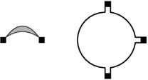
Figure 2: Graphical representation of the third cumulant. The notation is explained in LeDoussalWiesePREPg . The first diagram yields the terms proportinal to $I_{2}$, the second diagram the terms proportional to $I_{3}$ in Eq. (4.31).

Higher cumulants of the renormalized disorder can be obtained by the same method using (4.23) and its extensions. They can also be obtained by the graphical method. For simplicity here we give only the expression of the third cumulant. The complete expression for the fourth cumulant, together with all calculational details and an introduction to the graphical method, can be found in Appendix C.

The third cumulant is found to be:

$$\tilde{S}(x,y,z) = \frac{6TI_{2}}{1+4I_{2}\tilde{B}^{\prime\prime}(0)}\text{sym}_{x,y,z}\Big{[}\tilde{B}^{\prime}(x)\tilde{B}^{\prime}(y)\Big{]}$$ (4.31)

$$+24I_{3}\text{sym}_{x,y,z}\Big{[}(\tilde{B}^{\prime}(x)-\tilde{B}^{\prime}(0))\tilde{B}^{\prime}(x)\tilde{B}^{\prime}(y)\Big{]}$$

$$-8I_{3}\tilde{B}^{\prime}(y)\tilde{B}^{\prime}(z)\tilde{B}^{\prime}(x)\ ,$$

where $\text{sym}_{x,y,z}$ is $1/6$ times the sum of all permutations of $x,y,z$. Note that this relation is exact for all values of the mass $m$, and not just a fixed point form. The only input in the derivation is the absence of a third cumulant for the bare model ($m=\infty$). It would be interesting to include an additional bare third cumulant. The fourth cumulant is derived in appendix C, where also details for the graphical method are given.

V Graphical Interpretation

$\displaystyle\frac{1}{2}B^{\prime\prime}(v^{2})(v^{2})^{2}$         $\displaystyle\frac{1}{3!}B^{\prime\prime\prime}(v^{2})(v^{2})^{3}$         $TB^{\prime}(v^{2})$

Figure 4: Examples for vertices and the 1-loop tadpole diagram which is dominant at large $N$.

Figure 6: The four 1-loop diagrams correcting the disorder. A fat dot represents a vertex $B$, a solid line the field $u$, and its correlator. A dashed line attaches two fields $u$ to a vertex $B$. We do not draw replica-indices.

Figure 8: Loops which give additional factors of $1/N$, as explained in the main text.

Figure 10: Tree-configurations which contribute to $\tilde{B}(v^{2})$.

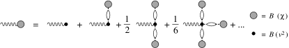
Figure 12: Self-consistent equation at leading order for $\tilde{B}^{\prime}(v_{ab}^{2})=B^{\prime}(\chi_{ab})$. The wiggly line denotes a derivative, and is combinatorially equivalent to choosing one $B$. At finite $T$ one can attach an additional arbitrary number of tadpoles to any $B$.

In this section, we sketch how the central results at large $N$ can be obtained graphically, first the saddle-point equation (4.29), which gives the effective disorder $\tilde{B}$ as a function of the bare disorder $B$, and second the $\beta$-function (6.9).

The graphical rules for the perturbation theory of the replicated model have been described in detail in LeDoussalWieseChauve2003 for $N=1$ and we refer the reader to this work for elementary details. Here there are in addition $N$ components of the field $u_{a}^{i}$, the propagator being diagonal in all indices. For the present purpose we are mostly interested in the counting in $N$, and since it is difficult to represent graphically both vector- and replica-indices, we work with unsplitted vertices (see LeDoussalWieseChauve2003 ) and specify the replica content only when needed. Disorder vertices may contain arbitrary number of derivatives and some examples are represented on Fig. 4. As usual there is a factor of $1/N$ per derivative (i.e. per dashed line) at each vertex (see e.g. Fig. 4, using $v^{2}=u^{2}/N$), $N$ per vertex, and $N$ per loop.

We consider the effective action, i.e. the sum of all 1-particle irreducible diagrams (1PI), and later focus on its 2-replica part. We start our analysis at $T=0$ with the three possible 1-loop diagrams, as presented on figure 6. They are obtained from contracting

$$\frac{N}{2}\sum_{ab}B\big{(}\textstyle\frac{(u^{a}_{x}-u^{b}_{x})^{2}}{N}\big{)}\ \displaystyle\frac{N}{2}\sum_{cd}B\big{(}\textstyle\frac{(u^{c}_{y}-u^{d}_{y})^{2}}{N}\big{)}\ .$$ (5.1)

In order to simplfy the calculation we omit the terms taken at coinciding replicas (e.g. $B^{\prime}(0)$), they can be added at the end. Contracting (5.1) twice between points $x$ and $y$ gives

$$\frac{N}{2}C_{xy}^{2}\sum_{ab}\! \bigg{[} \!B^{\prime}\big{(}\textstyle\frac{(u^{a}_{x}-u^{b}_{x})^{2}}{N}\big{)}B^{\prime}\big{(}\textstyle\frac{(u^{a}_{y}-u^{b}_{y})^{2}}{N}\big{)}$$ (5.2)

$$+\displaystyle\frac{2}{N}B^{\prime}\big{(}\textstyle\frac{(u^{a}_{x}-u^{b}_{x})^{2}}{N}\big{)}B^{\prime\prime}\big{(}\textstyle\frac{(u^{a}_{y}-u^{b}_{y})^{2}}{N}\big{)}\frac{(u^{a}_{y}-u^{b}_{y})^{2}}{N}$$

$$+\displaystyle\frac{2}{N}B^{\prime\prime}\big{(}\textstyle\frac{(u^{a}_{x}-u^{b}_{x})^{2}}{N}\big{)}\frac{(u^{a}_{x}-u^{b}_{x})^{2}}{N}B^{\prime}\big{(}\textstyle\frac{(u^{a}_{y}-u^{b}_{y})^{2}}{N}\big{)}$$

$$+\frac{4}{N}B^{\prime\prime}\big{(}\textstyle\frac{(u^{a}_{x}-u^{b}_{x})^{2}}{N}\big{)}\frac{(u^{a}_{x}-u^{b}_{x})^{2}}{N}B^{\prime\prime}\big{(}\textstyle\frac{(u^{a}_{y}-u^{b}_{y})^{2}}{N}\big{)}\frac{(u^{a}_{y}-u^{b}_{y})^{2}}{N}\bigg{]}$$

$$+\,\mbox{higher replica terms}$$

This is graphically depicted on figure 6. The important observation is that only the first diagram, with a closed $u$-loop is contributing in the limit of large $N$. This analysis can be repeated to higher loop order. Again, only diagrams as the first one on figure 6 contribute. Especially, there are no loops with three propagators or more, as loops 4 or 6 on figure 8. Also, there are no “meta-loops”, i.e. loops formed by loops, as loop 5 on figure 8. Finally, only diagrams as those on figure 10 survive, which as building block have only the elementary 1-loop diagram with a closed loop contributing a factor of $N$, as the first diagram on figure 6. These are tree-like diagrams, where the nodes are made out of $B$ and the links out of the before-mentioned 1-loop diagram (two parallel replica lines in the splitted diagrammatics LeDoussalWieseChauve2003 which produce the desired 2-replica term). At junction points the replica lines branch also in parallel. These are of course not tree diagrams, i.e. they are 1PI and contribute to the effective action. Note on Fig. 10 that since there is a $1/(2T^{2})$ factor per vertex, but that each vertex (except one) comes with two propagators (factor $T^{2}$) the counting in temperature is right to produce a 2-replica term with the expected $1/(2T^{2})$ global factor (the 3-replica terms proportional to $T$ have been discarded etc.).

We are now in a position to derive the self-consistent equation (4.29). The key-observation is that deriving $\tilde{B}(v^{2})$ once with respect to its argument, amounts in the graphical intepreation of figure 10 to choose one of the bare vertices $B(v^{2})$, and deriving it. $\tilde{B}^{\prime}(v^{2})$ thus is $B^{\prime}(v^{2})$, with as many branches attached as one wants. Every branch consists out of a 1-loop integral $\parbox{17.72939pt}{\hskip 3.44444pt\includegraphics[scale={0.25}]{./figures/1loop}\hskip 3.44444pt}=I_{2}$ times another tree; the latter is again $\tilde{B}(v^{2})$, given that one of the bare vertices is chosen, i.e. again $\tilde{B}^{\prime}(v^{2})$. Since attaching loops to $B^{\prime}(v^{2})$ amounts to deriving $B^{\prime}(v^{2})$ once for every loop, we arrive at

$$\tilde{B}^{\prime}(v^{2}) = \sum_{\ell=0}^{\infty}\frac{B^{(n+1)}(v^{2})\left[4I_{2}(\tilde{B}^{\prime}(v^{2})-\tilde{B}^{\prime}(0))\right]^{\ell}}{\ell!}$$ (5.3)

$$= B^{\prime}\!\left(v^{2}+4I_{2}[\tilde{B}^{\prime}(v^{2})-\tilde{B}^{\prime}(0)]\right)\ .$$

Note that we have added the term with coinciding replica-indices, dropped previously. The combinatorial factor comes from the expansion of the exponential function in ${\mathrm{e}}^{-\cal S}$. That it indeed resums to $B^{\prime}$ with a shifted argument is natural: For a function $f(x)$ taking the expectation value $\left<f(x)\right>$ in a theory with only a first moment $\left<x\right>$ is equivalent to calculating $f(\left<x\right>)$. Taylor-expanding the latter leads to the above combinatorics.

By the same arguments the full effective action can be written as the sum over tree-like (but not tree) diagrams represented in Fig. 10 where, in addition, each vertex can be dressed by an arbitrary number of tadpoles (see Fig.4). Each tadpole brings an additional factor of $T$, thus tadpoles contribute to the two replica term only at $T>0$. At finite temperature, any of the $v^{2}$’s could be contracted, leading to the relacement

$$(v^{a}-v^{b})^{2}\to(v^{a}-v^{b})^{2}+2TI_{1}\ .$$ (5.4)

(This offers another possibility to verify the combinatorics in 5.3.) Thus the final result is

$$\tilde{B}^{\prime}(v^{2})=B^{\prime}\!\left(v^{2}+2TI_{1}+4I_{2}[\tilde{B}^{\prime}(v^{2})-\tilde{B}^{\prime}(0)]\right)$$ (5.5)

We now illustrate how to recover the $\beta$-function. Applying $-m\partial/\partial m$ to $\tilde{B}$ implies to derive each integral w.r.t. $m$ appearing in each loop of Fig 10. Diagrammatically this amounts to choosing in the tree of Fig 10 one of the bonds (loop $I_{2}$) which connects two $B$’s. Summing over all trees, it gives a term

$$2\left(-m\frac{\partial}{\partial m}I_{2}\right)\left[\tilde{B}^{\prime}(v^{2})^{2}-2\tilde{B}^{\prime}(v^{2})\tilde{B}^{\prime}(0)\right]$$ (5.6)

since the two trees attached to the loop $I_{2}$ are nothing but $B(v^{2})$, derived once, and again itself with things attached, i.e. $\tilde{B}^{\prime}(v^{2})$ as given in (5.5). This reproduces the $T=0$ term in (6.9).

The second contribution comes from deriving $TI_{1}$. The graphical derivation is complicated, and we refer the interested reader to LeDoussalWiesePREPg where a more complete, but much more involved, diagrammatic method is presented.

VI Functional renormalization group equations

VI.1 From self-consistent to FRG equation

We will now study the self-consistent equation, exact for $N=\infty$, for the second cumulant correlator of the random potential that we have derived in the previous Section:

$$\tilde{B}^{\prime}(x)=B^{\prime}\Big{(}x+2TI_{1}+4I_{2}(\tilde{B}^{\prime}(x)-\tilde{B}^{\prime}(0))\Big{)}\ ,$$ (6.1)

which involves only the two one loop integrals:

$$I_{1} = \int_{0}^{\Lambda}\frac{d^{d}k}{(2\pi)^{d}}\frac{1}{k^{2}+m^{2}}$$ (6.2)

$$I_{2} = \int_{0}^{\Lambda}\frac{d^{d}k}{(2\pi)^{d}}\frac{1}{(k^{2}+m^{2})^{2}}\ ,$$ (6.3)

where we have indicated symbolically that a short scale UV cutoff is needed for $I_{2}$ to be finite if $d\geq 4$ and for $I_{1}$ for $d\geq 2$.

There is a simple way to obtain directly the solutions of (6.1) which we will detail below. It is also interesting to turn this equation into a FRG equation for the function $\tilde{B}(x)$ as a function of the scale parameter $m$. Indeed this yields the $\beta$-function of the field theory in the limit of infinite $N$, which is our main goal. Let us show first how one does it.

Let us first take a derivative of (6.1) with respect to $x$. One obtains:

$$\frac{\tilde{B}^{\prime\prime}(x)}{1+4I_{2}\tilde{B}^{\prime\prime}(x)}=B^{\prime\prime}\Big{(}x+2TI_{1}+4I_{2}(\tilde{B}^{\prime}(x)-\tilde{B}^{\prime}(0))\Big{)}\ .$$ (6.4)

Taking the derivative $m\partial_{m}$ of (6.1) and using (6.4) gives:

$$m\partial_{m}\tilde{B}^{\prime}(x) = \frac{\tilde{B}^{\prime\prime}(x)}{1+4I_{2}\tilde{B}^{\prime\prime}(x)}\Big{[}2m\partial_{m}TI_{1}$$ (6.5)

$$+4(m\partial_{m}I_{2})(\tilde{B}^{\prime}(x)-\tilde{B}^{\prime}(0))$$

$$+4I_{2}m\partial_{m}\tilde{B}^{\prime}(x)-4I_{2}m\partial_{m}\tilde{B}^{\prime}(0)\Big{]}\ .\qquad$$

Regrouping the terms one obtains:

$$m\partial_{m}\tilde{B}^{\prime}(x) = \tilde{B}^{\prime\prime}(x)\Big{[}2m\partial_{m}TI_{1}-4I_{2}m\partial_{m}\tilde{B}^{\prime}(0)$$ (6.6)

$$\hphantom{\tilde{B}^{\prime\prime}(x)\Big{[}}+4(m\partial_{m}I_{2})(\tilde{B}^{\prime}(x)-\tilde{B}^{\prime}(0))\Big{]}\ .\qquad$$

From (6.5) one also has

$$m\partial_{m}\tilde{B}^{\prime}(0)=\frac{\tilde{B}^{\prime\prime}(0)}{1+4I_{2}\tilde{B}^{\prime\prime}(0)}2m\partial_{m}(TI_{1})\ .$$ (6.7)

Inserting (6.7) into (6.6 ) finally yields

$$m\partial_{m}\tilde{B}^{\prime}(x) = \tilde{B}^{\prime\prime}(x)\Big{[}2(m\partial_{m}TI_{1})\frac{1}{1+4I_{2}\tilde{B}^{\prime\prime}(0)}$$ (6.8)

$$\hphantom{\tilde{B}^{\prime\prime}(x)\Big{[}}+4(m\partial_{m}I_{2})(\tilde{B}^{\prime}(x)-\tilde{B}^{\prime}(0))\Big{]}\ .\qquad$$

This equation is valid for any space dimension $d$. It can be integrated once w.r.t. $x$ to obtain the final result

$$m\partial_{m}\tilde{B}(x) = \frac{2(m\partial_{m}TI_{1})}{1+4I_{2}\tilde{B}^{\prime\prime}(0)}\tilde{B}^{\prime}(x)$$ (6.9)

$$+2(m\partial_{m}I_{2})\left[\tilde{B}^{\prime}(x)^{2}-2\tilde{B}^{\prime}(0)\tilde{B}^{\prime}(x)\right]\ ,\qquad$$

where we have dropped an $m$-dependent integration constant.

A general method to study (and solve) the FRG equation (6.8) is then to start from $m=\infty$ where the initial condition is $\tilde{B}(x)=B(x)$ in the presence of a UV momentum cutoff $\Lambda$, or a lattice with lattice constant $a=1/\Lambda$. Then one studies how $\tilde{B}(x)$ evolves as $m$ is slowly decreased.

There are thus two possible paths to solve the problem, namely the direct inversion of the self-consistent equation and the solution of (6.8) with the above initial condition. Both are studied below. These two methods are clearly equivalent when the solution $\tilde{B}(x)$ is analytic at $x=0$. Indeed, in the above derivation, we have assumed that $\tilde{B}^{\prime\prime}(0)$ exists. This will not always hold, as we now discuss. What the proper ensuing modifications are is a subtle point which will be examined later.

VI.2 General features: Analytic vs non-analytic solution

Before solving this equation let us first find the conditions under which there exists an analytic solution. This will give us insight in the phases of the model. One notes from (6.4) that:

$$\frac{1}{\tilde{B}^{\prime\prime}(0)}=\frac{1}{B^{\prime\prime}(2TI_{1})}-4I_{2}\ .$$ (6.10)

For $m=\infty$ the starting value is $\tilde{B}^{\prime\prime}(0)=B^{\prime\prime}(0)>0$, in any dimension $d$. (The force correlator decays for small distances.) As $m$ is decreased several things can happen.

Let us start with $T=0$. Then for $d<4$, since $I_{2}$ diverges for small $m$, one sees from (6.10) that $\tilde{B}^{\prime\prime}(0)$ becomes infinite as $m\to m_{c}^{+}$, where the Larkin mass $m_{c}$ is the solution of:

$$4S_{d}\int_{0}^{\Lambda}{\mathrm{d}}q\frac{q^{d-1}}{(q^{2}+m_{c}^{2})^{2}}=\frac{1}{B^{\prime\prime}(0)}$$ (6.11)

with $S_{D}=1/(2^{d-1}\pi^{d/2}\Gamma[d/2])$ and has the standard dependence $m_{c}\sim B^{\prime\prime}(0)^{1/\epsilon}$ of the inverse Larkin length on the bare disorder (a Larkin length $L_{c}=1/m_{c}$ can be defined). Since $\tilde{B}^{\prime\prime}(0)$ is like $\tilde{R}^{\prime\prime\prime\prime}(0)$ positive, this divergence is the usual one of the FRG, as also found in 1- and 2-loop studies DSFisher1986 ; BalentsDSFisher1993 ; BucheliWagnerGeshkenbeinLarkinBlatter1998 ; ChauveLeDoussalWiese2000a ; LeDoussalWieseChauve2002 ; ChauveLeDoussal2001 , where it signals that the function $\tilde{R}(u)$ becomes non-analytic and that a cusp singularity forms at $u=0$ in the second derivative $-\tilde{R}^{\prime\prime}(u)$, i.e. in the correlator of the pinning force. This is usually interpreted as a glass phase with many metastable states beyond the Larkin length. Thus for $d<4$ the function always becomes non-analytic at large scale (small mass), and there is a single glass phase. For $d>4$, since $I_{2}$ is convergent, the cusp occurs only if the bare disorder is sufficiently large.

At non-zero temperature $T>0$ (6.10) shows that for $2<d<4$ thermal fluctuations do not change the scenario. Since $I_{1}$ remains finite, temperature only slightly renormalizes the value of $m_{c}$ downward, as

$$4S_{d}\int_{0}^{\Lambda}{\mathrm{d}}q\frac{q^{d-1}}{(q^{2}+m_{c}^{2})^{2}}\approx\frac{1}{B^{\prime\prime}(2TS_{d}\Lambda^{d-2}/(d-2))}$$ (6.12)

for $\Lambda\gg m_{c}$. For $d<2$ the effect of thermal fluctuations is more important. For definiteness let us consider the set of models with power law correlations (2.10). Then (6.10) becomes:

$$\frac{1}{\tilde{B}^{\prime\prime}(0)}=\frac{1}{g\gamma}(a^{2}+2TI_{1})^{1+\gamma}-4I_{2}\ .$$ (6.13)

Since both integrals diverge for small mass as $I_{1}\sim 1/m^{2-d}$, $I_{2}\sim 1/m^{4-d}$, one can distinguish three cases:

• If disorder correlations decay fast enough $\gamma>\gamma_{c}(d)=2/(2-d)$ then the $I_{1}$ term wins and as $m\to 0$ one has $\tilde{B}^{\prime\prime}(0)\to 0$, indicating that disorder is subdominant, resulting in a high-temperature phase. In that case the solution is analytic as $m\to 0$. There is however a more complicated behavior for intermediate values of $m$ (see Appendix E).

• If disorder correlations decay slower, i.e. $\gamma<\gamma_{c}(d)$, the term proportional to $I_{2}$ wins and the solution always becomes non-analytic at some Larkin mass.

• In the marginal case, $\gamma=\gamma_{c}(d)$ there is a transition at some critical temperature $T_{c}$ between a high temperature phase and a glass phase.

These features are very general and each of these cases will be studied in more details below.

One can immediately see that the existence of an analytic solution for $\tilde{B}(u)$ is in one to one correspondence to the existence of a locally stable replica symmetric solution of the MP equations. Indeed the condition for the stability of the RS saddle point is precisely that the replicon eigenvalue be positive, namely that MezardParisi1991 :

$$\lambda_{\mathrm{rep}}(p) = 1-4I_{2}(p)B^{\prime\prime}(2TI_{1})$$ (6.14)

$$I_{2}(p) = \int_{k}(k^{2}+m^{2})^{-1}((k+p)^{2}+m^{2})^{-1}\qquad$$ (6.15)

be positive for all $p$. The RSB instability occurs when the lowest eigenvalue, which corresponds to $p=0$, vanishes. The condition $\lambda_{\mathrm{rep}}(p=0)=0$ is equivalent to the vanishing of (6.10), i.e. of the divergence of $\tilde{B}^{\prime\prime}(0)$ and the emergence of non-analytic behavior. Thus the generation of a cusp in the FRG coincides at large $N$ exactly with the instability of the RS solution.

It is easy to see that an analytic solution $\tilde{B}(x)$ of (6.1) and (6.8) cannot describe the glass phase at $T=0$. Indeed when $\tilde{B}(x)$ is analytic, Eq. (4.31) and similar results for higher cumulants indicate that the full effective action is analytic. It is then immediate to obtain correlations from its derivatives. For instance, from (2.36) the 2-point function at $q=0$ is simply:

$$\frac{1}{N}\left<u_{a}(q)\cdot u_{b}(q)\right>|_{q=0}=\frac{T}{m^{2}}\delta_{ab}-2\frac{\tilde{B}^{\prime}(0)}{m^{4}}$$ (6.16)

On the other hand, setting $x=0$ in (6.1) one finds:

$$\tilde{B}^{\prime}(0)=B^{\prime}(2TI_{1})\ .$$ (6.17)

Thus at $T=0$ one recovers the dimensional reduction (DR) result $\overline{u^{2}}\sim m^{-d-2\zeta}$ with $\zeta=\zeta_{\mathrm{DR}}=(4-d)/2$ instead of a non-trivial value for $\zeta$ expected in the glass phase. Furthermore since the effective action is analytic, all higher connected cumulants will trivially vanish at $T=0$ (or be equal to the bare ones if the bare model contains such higher cumulants) from the DR property. Clearly, in the glass phase, the DR scaling is expected to be incorrect and a non-analytic solution should be found, as well as a way to escape (6.17). Below we find how such a mechanism occurs within the FRG.

It will emerge from our study that for the case where disorder is relevant in the large scale limit (i.e. the long range case $\gamma<\gamma_{c}(d)$ mentioned above) the non-analytic solution of the FRG equation will correspond to the full replica symmetry breaking solution of MP. The situation for the short range case is more delicate. Both are discussed below.

VI.3 FRG equation for rescaled disorder, $d<4$

The equation (6.8) is valid (for $N=\infty$) in any spatial dimension $d$. Since one has the exact relation:

$$-\frac{1}{2}m\partial_{m}I_{1}=m^{2}I_{2}$$ (6.18)

one sees that the FRG equation (6.8) has a well defined limit $\Lambda\to\infty$ for $d<4$. It makes formulae somewhat simpler so we will start by considering this case; the case $d\geq 4$ will be studied later. Note that although the equation has a well-defined limit, its solution may require a UV cutoff (e.g. as is manifestly the case in integrating (6.18) above).

Thus from now on we study $d<4$ and consider the infinite UV cutoff limit. Then one has

$$I_{2}=A_{d}\frac{m^{-\epsilon}}{\epsilon}\ ,\qquad A_{d}=\frac{2}{(4\pi)^{d/2}}\Gamma(3-\frac{d}{2})$$ (6.19)

with $\epsilon=4-d$. It is convenient to define the rescaled dimensionless function:

$$b(x)=4A_{d}m^{4\zeta-\epsilon}\tilde{B}(xm^{-2\zeta})\ ,$$ (6.20)

where $\zeta$ is a fixed number, but for now arbitrary. Note that whether one works with $\tilde{B}$ or the rescaled $b(x)$ does not make any difference for the possibility of a non-analyticity or a divergence of the second derivative.

Then $b(x)$ satisfies the FRG equation in the infinite-$N$ limit:

$$-m\partial_{m}b(x) = \beta[b]$$

$$= (\epsilon-4\zeta)b(x)+2\zeta xb^{\prime}(x)$$

$$+\frac{1}{2}b^{\prime}(x)^{2}-b^{\prime}(x)b^{\prime}(0)+T_{m}\frac{b^{\prime}(x)}{1+\frac{b^{\prime\prime}(0)}{\epsilon}}+c_{m}\ .$$

The rescaled temperature, and the energy exponent $\theta$ are defined as

$$T_{m} = T\frac{4A_{d}}{\epsilon}m^{\theta}$$ (6.22)

$$\theta = d-2+2\zeta\ .$$ (6.23)

To obtain (LABEL:frg2) we have also integrated (6.8) once, so there is a priori a $m$-dependent integration constant.

We emphasize that this FRG equation (LABEL:frg2) that we have derived is valid, to dominant order in $1/N$, in any dimension $d<4$ and at any temperature $T$. In a previous study BalentsDSFisher1993 Balents and Fisher studied another limit: arbitrary $N$ but only to first order in $\epsilon=4-d$ and $T=0$. If we consider the dominant order in $N$ of their equation, we find that it is identical to the $T=0$ part of (LABEL:frg2) (up to some changes in notation). Equation (LABEL:frg2) however is valid to all orders in $\epsilon$, an important point which the method used in BalentsDSFisher1993 could not address. Comparison of (LABEL:frg2) to our recent 2-loop, i.e. $O(\epsilon^{2})$ studies requires to expand to next order in $1/N$ and is performed in LeDoussalWiesePREPg .

Furthermore (LABEL:frg2) includes the effect of temperature to all orders in $\epsilon$. Expanding the term proportional to $T$ to lowest order in disorder $b$, one finds the term $T_{m}b^{\prime}(x)$. This is the large-$N$ limit of the tadpole term obtained in the 1-loop FRG at $T>0$ Balents1993 ; ChauveGiamarchiLeDoussal1998 ; ChauveGiamarchiLeDoussal2000 ; MullerGorokhovBlatter2001 :

$$\partial_{l}\tilde{R}(u) = T\sum_{i=1}^{N}\partial_{i}^{2}\tilde{R}(u)$$

$$\to\partial_{l}B(v^{2}) = T\tilde{B}^{\prime}(v^{2})+\frac{T}{N}v^{2}\tilde{B}^{\prime\prime}(v^{2})\ ,$$ (6.24)

where for infinite $N$ the last term drops out. (It appears however to next order in $1/N$ LeDoussalWiesePREPg .)

The form and the effect of the temperature term in (LABEL:frg2) to all orders in $\epsilon$ is radically different from its 1-loop truncation. Indeed, in the 1-loop FRG the temperature is known to smoothen the cusp and render the function $\tilde{R}(u)$ analytic in a boundary layer $u\sim\tilde{T}_{m}$ (e.g. for $N=1$ Balents1993 ; ChauveGiamarchiLeDoussal2000 ; BalentsLeDoussal2002a ) with $\tilde{R}^{\prime\prime\prime\prime}(0)\sim 1/\tilde{T}_{m}$. Here however, as further analysis confirms below, for $\theta>0$ the divergence of $\tilde{b}^{\prime\prime}(0)$ is self-reinforcing since it kills the term proportional to $T_{m}$. We find that it usually occurs at a finite (Larkin) scale. In the marginal case $\theta=0$, we will find non-trivial analytic finite-temperature fixed points.

VII Detailed analysis of the FRG equations

VII.1 Inversion of self-consistent equation

Let us now show how one can invert the self-consistent equation (6.1). We first rewrite it in terms of the rescaled correlator

$$b^{\prime}(x) = 4A_{d}m^{2\zeta-\epsilon}$$

$$\times B^{\prime}\Big{(}m^{-2\zeta}(x+\frac{1}{\epsilon}(b^{\prime}(x)-b^{\prime}(0))+2TI_{1}m^{2\zeta})\Big{)}\ ,$$

where in the term proportional to temperature, for $d>2$ we mean $\lim_{\Lambda\to\infty}TI_{1}$ choosing a bare temperature $T\sim\Lambda^{(2-d)}$ (this choice is known to be necessary to give a universal and finite $\beta$ function, see e.g. the discussion in Ref. LeDoussalWiesePREPg ). One can of course keep an explicit $\Lambda$ dependence everywhere, but that leads to needless complications without changing the result.

The above equation (VII.1) is easily inverted into

$$x=m^{2\zeta}\Phi\Big{[}\frac{y}{4A_{d}m^{2\zeta-\epsilon}}\Big{]}+\frac{1}{\epsilon}(y-y_{0})-\tilde{T}_{m}\ ,$$ (7.2)

where we define

$$y = y(x)=-b^{\prime}(x)$$ (7.3)

$$y_{0} = -b^{\prime}(0)=-4A_{d}m^{2\zeta-\epsilon}\tilde{B}^{\prime}(0)$$ (7.4)

$$\tilde{T}_{m} = 2TI_{1}m^{2\zeta}$$ (7.5)

with $\tilde{T}_{m}=T_{m}/(2-d)$ for $d<2$, and $\Phi$ is the inverse function of $-B^{\prime}(x)$ i.e.

$$(-B^{\prime})(\Phi(y))=y\ .$$ (7.6)

This means in turn that the FRG equation (LABEL:frg2) is fully integrable, a feature not immediately obvious if one does not know that it originates from a self-consistent equation (an observation not made in Ref. BalentsDSFisher1993 ). To better understand this integrability property let us show that (LABEL:frg2) can be transformed into a linear equation. Let us first take a derivative of (LABEL:frg2) and express it in terms of the new function $y(x)$ (7.3)

$$-m\partial_{m}y=(\epsilon-2\zeta)y+2\zeta xy^{\prime}-y^{\prime}(y-y_{0})+T_{m}\frac{y^{\prime}}{1-\frac{y^{\prime}_{0}}{\epsilon}}\ ,$$ (7.7)

where we denote $y^{\prime}_{0}=y^{\prime}(0)$. Converting this into an equation for the inverse function $x(y)$ one finds:

$$m\partial_{m}x=(\epsilon-2\zeta)yx^{\prime}+2\zeta x-(y-y_{0})+\frac{T_{m}\epsilon x^{\prime}_{0}}{\epsilon x^{\prime}_{0}-1}$$ (7.8)

with $x^{\prime}_{0}=x^{\prime}(y_{0})$ . We have used that $m\partial_{m}y(x)=-y^{\prime}(x)m\partial_{m}x(y(x))$ and have canceled a factor of $\frac{1}{x^{\prime}(y)}$ on both sides. (The validity near $x=0$ beyond the Larkin length is reexamined below).

One recovers now that the general solution of this linear equation is (VII.1) since it is the sum of the general solution of the homogeneous part

$$x=m^{2\zeta}\phi[ym^{\epsilon-2\zeta}]\ ,$$ (7.9)

where $\phi$ is an arbitrary function, and of a particular solution

$$x=\frac{1}{\epsilon}(y-y_{0})-\tilde{T}_{m}\ .$$ (7.10)

The $y$ dependence obviously satisfies (7.8) and for the constant part to work we use:

$$-m\partial_{m}y_{0} = (\epsilon-2\zeta)y_{0}+T_{m}\frac{y^{\prime}_{0}}{1-\frac{y^{\prime}_{0}}{\epsilon}}$$ (7.11)

$$-m\partial_{m}\tilde{T}_{m} = -2\zeta\tilde{T}_{m}+T_{m}\ .$$ (7.12)

The first line comes from evaluating (7.7) at $x=0$ and assuming analyticity, i.e. that $\lim_{x\to 0}y^{\prime}(x)(y(x)-y_{0})=0$, and equality which will not work beyond the Larkin length ($m<m_{c}$), as found below.

Now that we have clarified the connections between the two approaches (self-consistent equation and FRG) we can try to find solutions valid in the small mass limit. To analyze the solutions of the large-$N$ FRG equation (VI.3), two approaches are legitimate, corresponding to different points of view. The first, natural in mean field, is exact integration. But then one discovers that the solution becomes non-analytic upon reaching the Larkin mass. It thus raises the non-trivial question on how to continue this solution beyond the Larkin length. Before doing so, we will first examine a second point of view, more familiar from standard RG arguments.

VII.2 The FRG point of view: Search for fixed points

The standard RG approach amounts to construct and compute the $\beta$-function of the theory, and then search for a fixed point (function) which describes the large scale physics. Usually, finding the basin of attraction of the fixed point, or relating arbitrary initial conditions to the final approach of the fixed point is an unmanageably difficult task. It is fortunately also besides the goal of the RG which is to compute universal large scale physics independently of the irrelevant details of the bare model. Here, however, because of the large-$N$ limit, we can integrate the RG flow exactly and in principle “solve” any bare model. Let us temporarily ignore this integrability feature and focus on finding the zeroes of the $\beta$-function.

The $\beta$-function was derived previously within an $\epsilon$ expansion and non-analytic fixed points were found to one loop DSFisher1986 ; BalentsDSFisher1993 ; GiamarchiLeDoussal1995 and also to two loops ChauveLeDoussalWiese2000a ; LeDoussalWieseChauve2003 ; ChauveLeDoussal2001 . In the latter case additional “anomalous” terms are present in the $\beta$-function for the non-analytic theory to be renormalizable and a meaningful fixed point to exist. Viewing the right hand side of (LABEL:frg2) as the large-$N$ limit of the true $\beta$-function, let us follow the same strategy and ask whether we can find non-trivial fixed points.

Let us study $T=0$ and use the equivalent linear form of the FRG equation. We want to find the solutions $y(x)$ of

$$(\epsilon-2\zeta)yx^{\prime}+2\zeta x-(y-y_{0})=0\ .$$ (7.13)

$y_{0}$ is a fixed number (we want to impose $y_{0}=y(0)$), since we are looking for a fixed point function. Keeping $y_{0}$ arbitrary, one first tries a linear solution $x=ay+b$ which yields $a=1/\epsilon$ and $b=-y_{0}/(2\zeta)$. Writing $x(y)=(y/\epsilon)-y_{0}/(2\zeta)+\phi(y)$ one finds a homogeneous equation for $\phi$ and thus

$$x(y)=\frac{y}{\epsilon}-\frac{y_{0}}{2\zeta}+\alpha y^{-\frac{2\zeta}{\epsilon-2\zeta}}\ .$$ (7.14)

Imposing now $y_{0}=y(0)$, i.e. $x(y_{0})=0$, fixes the value of $\alpha$ and one finds the family of zero temperature fixed point functions, parameterized by $\zeta$:

$$x=x^{*}(y)=\frac{y}{\epsilon}-\frac{y_{0}}{2\zeta}+\frac{\epsilon-2\zeta}{2\zeta\epsilon}y_{0}^{\frac{\epsilon}{\epsilon-2\zeta}}y^{-\frac{2\zeta}{\epsilon-2\zeta}}\ .$$ (7.15)

Since $x>0$, $y_{0}>0$ one must have $\frac{2\zeta}{\epsilon-2\zeta}>0$ and thus

$$0<\zeta<\frac{\epsilon}{2}\ .$$ (7.16)

The case $\zeta=\frac{\epsilon}{2}$ corresponds to a Larkin random force model. For the same reason, we must exclude the branch $y>y_{0}$ and thus $x^{*}(y)$ is given by the unique solution of (7.15) with $x>0$ and $0\leq y\leq y_{0}$. Finally, for $\zeta=0$ we find the fixed point:

$$x=x^{*}(y)=\frac{1}{\epsilon}(y-y_{0}-y_{0}\ln(y/y_{0}))\ .$$ (7.17)

An important observation is that all of these fixed points exhibit automatically the expected cusp. Indeed one finds that $x^{\prime}(y_{0})=0$, i.e. $x(y)$ in (7.15) vanishes and has a minimum at $y=y_{0}$:

$$x^{*}(y)=\frac{1}{2(\epsilon-2\zeta)y_{0}}(y-y_{0})^{2}+O((y-y_{0})^{3})\ .$$ (7.18)

This gives

$$\tilde{b}^{\prime}(x)=\tilde{b}^{\prime}(0)+A\sqrt{x}+O(x)\ ,$$ (7.19)

with $A=\sqrt{2(\epsilon-2\zeta)|\tilde{b}^{\prime}(0)|}$, implying that the second derivative diverges as $x\to 0^{+}$

$$\tilde{b}^{\prime\prime}(x)\sim\frac{A}{2\sqrt{x}}+O(x^{0})\ .$$ (7.20)

Recalling that $y=-b^{\prime}(x)$ we see that all fixed points with $\zeta>0$ correspond to a power-law long-range correlator $b(x)$, while $\zeta=0$ corresponds to a gaussian short range disorder. If we follow the standard RG arguments, we can now sort the models (2.6) into these universality classes. Since for the bare model

$$B^{\prime}(z)\sim z^{-\gamma}\ ,$$ (7.21)

and since the decay of $R(u)$ in (2.6) at large $u$ can be argued to be identical for $B$ and $\tilde{B}$ (for LR fixed points) we find

$$\zeta=\zeta(\gamma)=\frac{4-d}{2(1+\gamma)}$$ (7.22)

or $\zeta=0$ for short range correlations. These values are valid to dominant order in $1/N$. In BalentsDSFisher1993 the effect of the $O(1/N)$ terms in the 1-loop FRG equation was studied, i.e. the corrections of $\zeta$ were estimated to order $O(\epsilon)$ and at zero temperature. For SR disorder it was found that the result of the GVM (i.e. Flory) is corrected by terms $a_{N}$ exponentially small in $N$, i.e.  $\zeta_{\mathrm{SR}}=\zeta(\gamma=\frac{N}{2}+1)+a_{N}\epsilon+O(\epsilon^{2})$. For LR disorder with $\gamma>\gamma^{*}(N)$ the result (7.22) was found to be uncorrected to $O(\epsilon)$. (The crossover SR to LR occurs at $\gamma^{*}$ such that $\zeta(\gamma^{*})=\zeta_{\mathrm{SR}}$). One can in fact argue that (7.22) is always exact in the LR case (see e.g. discussion in Ref. LeDoussalWieseChauve2003 ).

Several important remarks are in order. First we have found the fixed points of the inverted linear form (7.8) of the FRG equation. A valid question is whether this is equivalent to finding the fixed points of the initial form of the $\beta$-function (LABEL:frg2). Second we have found fixed points assuming that $m\partial_{m}y_{0}=0$. Since this is different from what has been found previously in (7.11) at $T=0$, one can ask whether these result are compatible.

These two questions have a common answer. Examining more closely what has really been done in this Section, we note that it is equivalent to declaring both (LABEL:frg2) and (7.8) valid for any $x>0$ and interpreting everywhere $y_{0}=y(0^{+})$ in (7.8) and, equivalently $b^{\prime}(0)$ as $b^{\prime}(0^{+})$ defined by continuity as $x\to 0^{+}$. This is legitimate since the transformation from (LABEL:frg2) to (7.8) is certainly valid for $x>0$ and we note that this answer the second question above since Eq. (7.7), i.e. the derivative of (LABEL:frg2), evaluated at $x\to 0^{+}$ yields:

$$-m\partial_{m}y(0^{+})=(\epsilon-2\zeta)y(0^{+})-\lim_{x\to 0^{+}}y^{\prime}(x)(y(x)-y^{\prime}(0^{+}))\ ,$$ (7.23)

which works both in the regime $m>m_{c}$ where the solution is analytic $y(0^{+})=y(0)$ and in the fixed point regime $m\to 0$ when the cusp has developed and the last term in (7.23) has a non-zero limit according to (7.19,7.20).

We expect these fixed points to be the physically correct solutions at small $m$. We now investigate whether we can confirm this by providing the solution at infinite $N$, for arbitrary mass $m$, i.e continue our solution (VII.1) beyond the Larkin length.

VII.3 Full solution beyond the Larkin mass

We now show that one can connect the two regimes, i.e. the regime for $m>m_{c}$ where an analytic solution exists to the asymptotic one, for $m\to 0$, studied in the previous Section. This can be done here because of the full integrability of the infinite-$N$ limit and provides a rare and non-trivial insight into what happens around the Larkin scale.

It is instructive to start our analysis with the specific power law models with LR correlations (2.10), together with the case of SR correlations (2.9), in the form of a Gaussian. The solution for an arbitrary bare potential $B(z)$ is more subtle, and will be given in Section VIII.4, and appendix H.

For the power law correlators the inverse function in (VII.1) is:

$$-B^{\prime}(z)=\frac{g}{(a^{2}+z)^{\gamma}}\quad\Leftrightarrow\quad z=\Phi(y)=\Big{(}\frac{y}{g}\Big{)}^{-1/\gamma}-a^{2}\ .$$ (7.24)

For gaussian correlations it is:

$$-B^{\prime}(z)=ge^{-z}\quad\Leftrightarrow\quad z=\Phi(y)=\ln(g/y)\ .$$ (7.25)

We can now insert this result into the general solution (7.2) of the self-consistent equation. $\zeta$ is arbitrary, but the convenient choice (to later obtain a fixed point) is $\zeta=\zeta(\gamma)$ such that the $m$ dependence of the first term drops. Let us define

$$\tilde{g}=4A_{d}g\ .$$ (7.26)

We then obtain, for power law models:

$$x = \left(\frac{y}{\tilde{g}}\right)^{-1/\gamma}+\frac{1}{\epsilon}(y-y_{0})-m^{2\zeta}a^{2}-\tilde{T}_{m}\qquad\quad$$ (7.27)

$$-b^{\prime}(0) = y_{0}=\tilde{g}(m^{2\zeta}a^{2}+\tilde{T}_{m})^{-\gamma}\ ,$$ (7.28)

since we want $y(0)=y_{0}$ i.e. $x(y_{0})=0$. This solution is valid for $m>m_{c}$ and the value of $b^{\prime}(0)$ is the DR result (6.17). For short range disorder the solution for $m>m_{c}$ is

$$x = \ln(\tilde{g}m^{-\epsilon}/y)+{\epsilon}^{{-1}}(y-y_{0})-\tilde{T}_{m}\qquad$$ (7.29)

$$-b^{\prime}(0) = y_{0}=\tilde{g}m^{-\epsilon}{\mathrm{e}}^{-\tilde{T}_{m}}\ ,$$ (7.30)

having set $\zeta=0$ in that case. We recall that $y(x)=-b^{\prime}(x)$. Note that the bare disorder is recovered for $m\to\infty$. We have kept temperature, but here we discuss only the case where

$$\theta=\theta(\gamma)=d-2+2\zeta(\gamma)>0\ ,$$ (7.31)

i.e. $2<d<4$, or $d<2$ with $\gamma<\gamma_{c}(d)=2/(2-d)$. In that case $\tilde{T}_{m}$ decreases as $m$ decreases, and, as mentioned above the role of temperature is minor.

Let us plot the r.h.s of (7.27), (7.29) on Fig. 14. The curve $x(y)$ has the indicated shape in all cases. It cuts the axis $x=0$ at $y=y_{0}$ and has a minimum $x^{\prime}(y_{c})=0$ at $y=y_{c}$ with

$$y_{c}=\tilde{g}^{1/(1+\gamma)}(\epsilon/\gamma)^{\gamma/(1+\gamma)}\ ,$$ (7.32)

independent of $m$, and $y_{c}=\epsilon$ for SR disorder. For $m>m_{c}$ the minimum occurs at negative $x$ and the slope at $y=y_{0}<y_{c}$ is non-zero, indicating an analytic solution $y(x)=-b^{\prime}(x)$. For large $m$ only the first term on the r.h.s. of (7.2) contributes and one recovers essentially the bare disorder $B$. Decreasing $m$ simply amounts to translate the curve upward along positive $x$, and $y_{0}$ increases as the curve $x(y)$ cuts the axis $x=0$ closer to the minimum. It reaches it at the Larkin mass, solution of $y_{0}=y_{c}$, i.e.

$$m_{c}^{2\zeta}a^{2}+\tilde{T}_{m_{c}}=(\tilde{g}\gamma/\epsilon)^{1/(1+\gamma)}=:\tilde{T}_{c}\ .$$ (7.33)

For SR disorder $y_{0}=y_{c}=\epsilon$ gives $m_{c}^{\epsilon}=\tilde{g}/\epsilon$. Exactly as $m\to m_{c}^{+}$ the solution acquires a cusp and one finds:

$$b^{\prime}(x)-b^{\prime}(0)\approx\sqrt{-2(\epsilon-2\zeta)b^{\prime}(0)x}$$ (7.34)

i.e. the same result as (7.19).

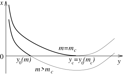
Figure 14: The function $x(y)$ given by (7.27) or (7.29). The physical branch is the one with $y<y_{0}$.

Although it is a priori not obvious how to follow this solution for $m<m_{c}$, the following remarkable property indicates how to proceed. If we compute the $\beta$-function, i.e. the r.h.s. of (7.8) using (7.27) at $m=m_{c}$ and $\zeta=\zeta(\gamma)$ we find that it exactly vanishes. Similarly the $\beta$-function for $b^{\prime}(x)$ also exactly vanishes for all $x>0$ provided we use also (7.23), i.e all $b^{\prime}(0)$ are defined as $b^{\prime}(0^{+})$. Thus at $m=m_{c}$ the function has already reached its fixed point form $x=x^{*}(y)$, and freezes for $m<m_{c}$. For the disorder correlators studied here, $b(x)$ evolves according to (7.27) or (7.29) until $m_{c}$ where it reaches its fixed point $b=b^{*}(x)$, and does not evolve for $m<m_{c}$. In particular $y_{0}=-b^{\prime}(0^{+})$ freezes at $m_{c}$ and one has $-m\partial_{m}y_{0}=0$ for $m<m_{c}$, exactly as was discussed in the previous Section.

The solution for $m<m_{c}$ is thus:

$$x = (y/\tilde{g})^{-1/\gamma}+{\epsilon}^{{-1}}(y-y_{0})-\tilde{T}_{c}\quad m<m_{c}$$

$$-b^{\prime}(0^{+}) = y_{0}=\tilde{g}\tilde{T}_{c}^{-\gamma}\ ,$$ (7.35)

where the parameter $\tilde{T}_{c}$ is defined in (7.33), thus it exactly identifies with the zero temperature fixed point (7.15) with $\zeta=\zeta(\gamma)$, as can be explicitly verified. This is easily understood a posteriori, since the same functions appear and in both cases we have two conditions to fix the two undetermined amplitudes $x(y_{0})=x^{\prime}(y_{0})=0$. It does however heavily rely on the exact power law form of the model, so it is not immediately obvious how it will extend to an arbitrary bare model $B(z)$. One clearly cannot expect in the general case that convergence to the fixed point will be completed within a finite scale. The solution to this puzzle is given below.

Similarly the solution for the Gaussian SR disorder correlator for $m\leq m_{c}$ is given by setting $m=m_{c}$ in (7.29), (7.30) with $y_{0}=\epsilon$ (which determines $m_{c}$).

The result of this section thus provides unambiguously a solution beyond the Larkin scale which connects with the zero temperature fixed point. It justifies the previous Section and the value obtained for $\zeta$. We found that for power law and gaussian models the freezing mechanism apparent in (7.23) leads to:

$$-m\partial_{m}y(0^{+}) = (\epsilon-2\zeta)y(0^{+})\quad,\quad m>m_{c}\qquad$$ (7.36)

$$-m\partial_{m}y(0^{+}) = 0~{}~{}~{}~{}~{}~{}~{}~{}~{}~{}~{}~{}~{}~{}~{}~{}~{}~{}~{}~{}~{}~{}\quad,\quad m<m_{c}\ .$$ (7.37)

The fixed point is reached at $m=m_{c}$.

VII.4 Role of temperature

In the case where disorder is relevant i.e. for $\theta(\gamma)>0$ (i.e. $2<d<4$; $d<2$ for $\gamma<\gamma_{c}=2/(2-d)$) we found in the previous Section that temperature plays only a minor role since the convergence to the non analytic zero temperature fixed point occurs on a finite (Larkin) RG scale. Whether it should be called a zero temperature fixed point can also be debated since it is reached when $T_{m}=T_{m_{c}}$. A proper definition of the renormalized temperature may then include the denominator in (LABEL:frg2).

Let us now examine the marginal case $\theta(\gamma)=0$, $\gamma=\gamma_{c}(d)$ and $d=2$ for SR disorder. We give here the main results, further details are examined in the Appendix F

The analytic solution is given by (7.27) and $y_{0}$ given by (7.28), where here $\tilde{T}_{m}=4A_{d}T/(\epsilon(2-d))$ does not flow as $m$ is lowered. Let us examine the second derivative,

$$\frac{1}{\tilde{b}^{\prime\prime}(0)} = -x^{\prime}(y_{0})=\frac{1}{\gamma y_{0}}\left(\frac{\tilde{g}}{y_{0}}\right)^{\!\!\frac{1}{\gamma}}-\frac{1}{\epsilon}$$ (7.38)

$$= \frac{1}{\epsilon}\left[\left(\frac{T}{T_{c}}m^{\theta}+\frac{a^{2}m^{2\zeta}}{\tilde{T}_{c}}\right)^{1+\gamma}-1\right]\ ,$$

which is a rescaled version of (6.13). The first line in (7.38) holds more generally (in the infinite UV cutoff limit) and to obtain the second we have set $\zeta=\zeta(\gamma)$, $\theta=\theta(\gamma)$ and assumed $d<2$. Setting now $\gamma=\gamma_{c}$, i.e. $\theta=0$, we find that there is a transition at a temperature $T=T_{c}$ defined by

$$T_{c}=\frac{\epsilon(2-d)}{4A_{d}}\tilde{T}_{c}=\frac{\epsilon(2-d)}{4A_{d}}(\tilde{g}\gamma/\epsilon)^{1/(1+\gamma)}\ ,$$ (7.39)

such that for $T>T_{c}$ the solution is analytic for all $m$ down to $m=0$, given by (7.27) and $\tilde{b}^{\prime\prime}(0)$ remains finite and given by (7.38). This is a line of analytic fixed points which terminates at $T_{c}$. For $T<T_{c}$ the solution freezes as in the previous Section, and becomes non-analytic at and below the Larkin mass

$$a^{2}m_{c}^{2\zeta}=\tilde{T}_{c}\left(1-\frac{T}{T_{c}}\right)\ .$$ (7.40)

The case $d=0$, $\gamma=1$ corresponds to the logarithmically correlated disorder $B(z)=-g\ln(a^{2}+z)$. It has been studied for finite $N$ in CarpentierLeDoussal2001 where it was shown that there is a transition for any $N$ at $T_{c}=\sqrt{g}$ ($g=\sigma/N$ in the notations of Ref.  CarpentierLeDoussal2001 ). The above result is in agreement with this value for $T_{c}$. There, for $N=1,2$ there is also a line of fixed points for $T>T_{c}$ with a continuously varying dynamical exponent (and also one for $T<T_{c}$ with a different dynamical exponent and some form of RSB). Since the dynamical exponent is perturbatively related to $\tilde{b}^{\prime\prime}(0)$, obtained above for infinite $N$, it would be particularly interesting to study the $1/N$ corrections in this case.

Let us now examine the case of SR disorder (2.9) in $d=2$. More details are given in the Appendix F. One has $\tilde{T}_{m}=2TI_{1}=(T/\pi)\ln(\Lambda/m)$. The analytic solution (7.29), (7.30) becomes

$$x = \ln(y_{0}/y)+{\epsilon}^{{-1}}(y-y_{0})$$ (7.41)

$$y_{0} = \tilde{g}m^{T/\pi-\epsilon}\Lambda^{-T/\pi}$$ (7.42)

with $\epsilon=2$. Thus there is a transition at $T=T_{c}=2\pi$. For $T<T_{c}$, we find $y_{0}$ to increase as $m$ decreases and reach $y_{0}=\epsilon$ at the Larkin mass. For $m<m_{c}$ the solution remains frozen to (7.41) with $y_{0}=\epsilon$. For $T>T_{c}$, we find that $y_{0}$ flows to zero and disorder is irrelevant. The physics is the same as the one contained in the variational method for the periodic model in $d=2$ GiamarchiLeDoussal1995 which exhibits a (so-called marginal) 1-step RSB solution.

The case $\gamma>\gamma_{c}(d)$, ($d<2$) is discussed in Appendix E. Although an analytic solution exists as $m\to 0$ and disorder is formally irrelevant, there are some freezing phenomena at intermediate $m$. It corresponds to the case where MP find, in addition to a RS solution, a 1-step RSB solution which is so called non-marginal (different in nature from the one step solutions obtained in the case $\theta=0$).

VIII Comparison between the RSB and the FRG approach

In this Section we compare the FRG approach at large $N$ with the GVM using RSB. Since the two methods study the same model in the same limit (large $N$) a precise connection should exist.

We start by comparing the two methods at the level of the results of the calculations. We first perform the comparison for power law models. Then we generalize the FRG solution to arbitrary bare disorder correlator. Based on these results, we address the deeper connections between the two methods, and emphasize what we learn from them about the physical consequences.

VIII.1 Zero momentum correlation function from the FRG

Our main result up to now is a non-trivial solution for the renormalized disorder correlator $\tilde{B}(z)$ as a function of the scale parameter $m$, i.e. the effective action for the zero momentum mode. Since this function is once differentiable, i.e. $\tilde{B}(z)=\tilde{B}(0)+\tilde{B}^{\prime}(0)z+O(z^{3/2})$, we can extract from its first derivative the 2-point correlation function at zero momentum (see Section II.2.2):

$$\langle v_{a}(q)\cdot v_{b}(q^{\prime})\rangle = \frac{1}{N}\langle u_{a}(q)\cdot u_{b}(q^{\prime})\rangle$$ (8.1)

$$= G_{ab}(q)(2\pi)^{d}\delta^{d}(q+q^{\prime})$$

$$G_{ab}(q=0) = \frac{T}{m^{2}}\delta_{ab}-2\frac{\tilde{B}^{\prime}(0)}{m^{4}}$$ (8.2)

$$= \frac{T}{m^{2}}\delta_{ab}-\frac{b_{m}^{\prime}(0)}{2A_{d}}m^{-d-2\zeta}\ ,$$

where in the last equation we have used the definition (6.20) for the rescaled function $b$, and added the index $m$ to recall its dependence on the mass.

In the case $\theta>0$, for the power-law models (2.10), we thus find, using $b_{m}^{\prime}(0)=-y_{0}$ from (7.28)

$$G_{a\neq b}(q=0) = 2g(m_{c}^{2\zeta}a^{2}+\tilde{T}_{m_{c}})^{-\gamma}m^{-d-2\zeta}$$ (8.3)

$$= \frac{1}{2A_{d}}\tilde{g}^{\frac{1}{1+\gamma}}\left(\frac{\epsilon}{\gamma}\right)^{\frac{\gamma}{1+\gamma}}m^{-d-2\zeta}\ ,$$

and, for $m>m_{c}$ the DR result (6.16), (6.17) (where $m_{c}$ is determined by (7.33)) and, we recall, $\zeta=\epsilon/(2(1+\gamma))$.

VIII.2 Explicit full RSB solution at large $N$

Let us recall the RSB solution at large $N$ and resolve carefully the MP saddle-point equation in presence of a mass. We only assume that there is indeed full RSB, to be checked a posteriori. Let us first reexpress the general solution, valid for an arbitrary $B$, in a rather compact form.

In the RSB method one first parameterizes the correlation matrix as $G_{ab}(k)=G(k,{\sf u})$ and the self-energy matrix $TG_{ab}^{-1}(k)-(k^{2}+m^{2})\delta_{ab}=\sigma_{ab}=\sigma({\sf u})$, in terms of the overlap $0<{\sf u}<1$ between (distinct) replicas $a$ and $b$ (and denote $\tilde{G}=G_{aa}$). The saddle point equations then read

$$\sigma({\sf u}) = -\frac{2}{T}B^{\prime}(\tilde{\chi}({\sf u}))$$ (8.4)

$$\tilde{\chi}({\sf u}) = 2\int_{k}(\tilde{G}(k)-G(k,{\sf u}))$$ (8.5)

$$= \tilde{\chi}({\sf u}^{c})+\int_{\sf u}^{{\sf u}^{c}}{\mathrm{d}}{\sf w}\int_{k}\frac{2T\sigma^{\prime}({\sf w})}{(k^{2}+m^{2}+[\sigma]({\sf w}))^{2}}\qquad$$

$$\tilde{\chi}({\sf u}^{c}) = 2T\int_{k}\frac{1}{k^{2}+m^{2}+\Sigma_{c}}$$ (8.6)

with

$$[\sigma]({\sf u})={\sf u}\sigma({\sf u})-\int_{0}^{\sf u}{\mathrm{d}}{\sf w}\,\sigma({\sf w})$$ (8.7)

and $\Sigma^{c}=[\sigma]({\sf u}\geq{\sf u}_{c})$. The last two equations are the RSB-matrix inversion formulae; $\sigma({\sf u})$ is assumed to be continuous. Taking a derivative of (8.4) w.r.t. $\sf u$ gives

$$\sigma^{\prime}({\sf u})=\sigma^{\prime}({\sf u})\,4B^{\prime\prime}(\tilde{\chi}({\sf u}))\int_{k}\frac{1}{(k^{2}+m^{2}+[\sigma]({\sf u}))^{2}}\ .$$ (8.8)

This equation admits two solutions: Either $\sigma({\sf u})$ is constant, or satisfies the marginality condition

$$1=4B^{\prime\prime}(\tilde{\chi}({\sf u}))\int_{k}\frac{1}{(k^{2}+m^{2}+[\sigma]({\sf u}))^{2}}\ .$$ (8.9)

We thus look for a solution of the full RSB equations (see Fig. 16) with a non-trivial function $\sigma({\sf u})$ for ${\sf u}_{m}<{\sf u}<{\sf u}_{c}$ joined by two plateaus

$$\sigma({\sf u}) = \sigma({\sf u}_{c})\ ,~{}\,\qquad{\sf u}\geq{\sf u}_{c}$$ (8.10)

$$\sigma({\sf u}) = \sigma(u_{m})\ ,\qquad{\sf u}\leq{\sf u}_{m}\ .$$ (8.11)

Similar forms are valid for $G(k,{\sf u})$ and $\tilde{\chi}({\sf u})$. The breakpoint ${\sf u}_{c}$ is related to the physics at the Larkin scale $m_{c}$, which, at weak disorder, can be much smaller than the UV scale $\Lambda$, while ${\sf u}_{m}$ depends on the IR cutoff $m$. (8.9) also yields by continuity a closed equation which determines $\Sigma_{c}$

$$1=4B^{\prime\prime}\left(2T\int_{k}\frac{1}{(k^{2}+m^{2}+\Sigma^{c})}\right)\int_{k}\frac{1}{(k^{2}+m^{2}+\Sigma^{c})^{2}}\ ,$$ (8.12)

as well as

$$1=4I_{2}B^{\prime\prime}(\tilde{\chi}({\sf u}_{m}))\ ,$$ (8.13)

since $[\sigma]({\sf u})=0$ for ${\sf u}\leq{\sf u}_{m}$. To solve these equations one firsts determines the function $[\sigma]({\sf u})$ (see below), then finds ${\sf u}_{c}$ and ${\sf u}_{m}$.

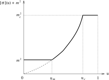
Figure 16: Full RSB solution for the function $[\sigma]({\sf{\sf u}})+m^{2}$ and a finite mass $m$. $\sigma({\sf u})$ has identical behavior, with two plateaus at values $\sigma({\sf u}=0)$ and $\sigma({\sf u}={\sf u}_{c})$. In both cases, upon increasing the mass only, ${\sf u}_{m}$ varies (increases) and the lower plateau moves up, the rest of the function being unchanged, see Eqs. (8.51) f. in the text. The dashed line is the zero mass solution. The lower breakpoint ${\sf u}_{m}$ reaches the upper one ${\sf u}_{c}$ at the Larkin mass $m=m_{c}$ above which the solution becomes RS. The FRG gives exactly the lower plateau value for $\sigma({\sf u}=0)=\sigma({\sf u}={\sf u}_{m})$ and its $m$-dependence. From it, the full RSB solution can be reconstructed, see Section VIII.5.

One can already note at this stage that (8.12) is exactly the condition (6.12) which determines the Larkin mass $m_{c}$, equivalent to the vanishing of the replicon:

$$\Sigma_{c}=m_{c}^{2}-m^{2}\qquad\mbox{for}\ m<m_{c}$$ (8.14)

and $\Sigma_{c}=0$ (no RSB) for $m>m_{c}$.

To find $[\sigma]({\sf u})$ for arbitrary $B$ and cutoff, one notes GiamarchiLeDoussal1995 that with the help of (8.9) and (8.4) $\sigma$ can be expressed as a function of $[\sigma]$ as

$$\sigma({\sf u})=-\frac{2}{T}B^{\prime}\left((B^{\prime\prime})^{-1}\bigg{(}\frac{1}{4\int_{k}\frac{1}{(k^{2}+m^{2}+[\sigma]({\sf u}))^{2}}}\bigg{)}\right)\ ,$$ (8.15)

where $(B^{\prime\prime})^{-1}$ is the inverse function of $B^{\prime\prime}$. Then one notes that $\sf u$ as a function of $\sigma$ of $[\sigma]$ is from (8.7) simply $1/{\sf u}={\mathrm{d}}\sigma/{\mathrm{d}}[\sigma]$. This yields immediately, using the chain rule:

$${\sf u} = -4T\,\frac{\big{[}\int_{k}\frac{1}{(k^{2}+m^{2}+[\sigma]({\sf u}))^{2}}\big{]}^{3}}{\int_{k}\frac{1}{(k^{2}+m^{2}+[\sigma]({\sf u}))^{3}}}$$ (8.16)

$$\times B^{\prime\prime\prime}\left((B^{\prime\prime})^{-1}\bigg{(}\frac{1}{4\int_{k}\frac{1}{(k^{2}+m^{2}+[\sigma]({\sf u}))^{2}}}\bigg{)}\right)\ .\qquad$$

Upon inversion one obtains the exact function $[\sigma]({\sf u})$, and inserting into (8.15) $\sigma({\sf u})$. More precisely, we see that the sum $[\sigma]({\sf u})+m^{2}$ is a $m$-independent function of ${\sf u}$, and thus from (8.15) $\sigma({\sf u})$ is also $m$-independent. Then one solves the self-consistent equation (8.12) for $\Sigma_{c}$, and finally obtains ${\sf u}_{c}$ from the above. The result can be written using (8.12) in the simple form

$${\sf u}_{c}=-4T\frac{\big{[}\int_{k}\frac{1}{(k^{2}+m^{2}_{c})^{2}}\big{]}^{3}}{\int_{k}\frac{1}{(k^{2}+m^{2}_{c})^{3}}}~{}~{}B^{\prime\prime\prime}\left((B^{\prime\prime})^{-1}\bigg{(}\frac{1}{4\int_{k}\frac{1}{(k^{2}+m^{2}_{c})^{2}}}\bigg{)}\right)\ .$$ (8.17)

Thus ${\sf u}_{c}$ depends only on the Larkin mass and is independent of $m$ (See appendix G for another derivation and a discussion of this useful property). Similarly one obtains:

$${\sf u}_{m} = -4T\frac{I_{2}^{3}}{I_{3}}B^{\prime\prime\prime}\left((B^{\prime\prime})^{-1}\bigg{(}\frac{1}{4I_{2}}\bigg{)}\right)$$

$$I_{3} = \int_{k}\frac{1}{(k^{2}+m^{2})^{3}}\ .$$ (8.18)

Let us apply these considerations to the power law model (2.10). For this model the Larkin mass is determined by (7.33). Next one has:

$$B^{\prime\prime\prime}\left((B^{\prime\prime})^{-1}(y)\right)=-\frac{\tilde{g}\gamma(1+\gamma)}{4A_{d}}\left(\frac{4A_{d}y}{\gamma\tilde{g}}\right)^{\frac{2+\gamma}{1+\gamma}}\ .$$ (8.19)

In the limit of infinite UV cutoff $\Lambda$ limit, using $I_{2}=(m^{2})^{-\epsilon/2}A_{d}/\epsilon$ and $I_{3}=(m^{2})^{-1-\epsilon/2}A_{d}/4$ we obtain from (8.16)

$$m^{2}+[\sigma]({\sf u}) = (\tilde{A}{\sf u})^{2/\theta}$$ (8.20)

$$\tilde{A} = \frac{1}{4TA_{d}(1+\gamma)}\epsilon^{\frac{1+2\gamma}{1+\gamma}}(\gamma\tilde{g})^{\frac{1}{1+\gamma}}\qquad$$ (8.21)

$${\sf u}_{m} = m^{\theta}/\tilde{A}$$ (8.22)

$${\sf u}_{c} = m_{c}^{\theta}/\tilde{A}$$ (8.23)

with $\theta=d-2+2\zeta$, $\zeta=\epsilon/(2(1+\gamma))$. Using (8.15) one finds the $m$-independent result

$$\sigma({\sf u})=\frac{2}{2-\theta}\tilde{A}^{2/\theta}{\sf u}^{-1+\frac{2}{\theta}}\ .$$ (8.24)

In particular one has the value of the lower plateau (see Fig. 16)

$$\sigma_{m}(0)=\sigma({\sf u}_{m})=\frac{2}{2-\theta}\frac{m^{2}}{{\sf u}_{m}}=\frac{2}{2-\theta}\tilde{A}m^{2-\theta}$$ (8.25)

Let us already note the relation ${\sf u}_{m}\partial_{m^{2}}\sigma_{m}(0)=1$ which will be demonstrated to hold more generally below.

VIII.3 Correlation function in MP solution compared to FRG

The inversion formula yielding the diagonal correlation from the RSB solution is

$$G_{aa}(q=0)=\frac{T}{m^{2}}\left[1+\frac{\sigma_{m}(0)}{m^{2}}+\int_{{\sf u}_{m}}^{1}\frac{{\mathrm{d}}{\sf u}}{{\sf u}^{2}}\frac{[\sigma]({\sf u})}{m^{2}+[\sigma]({\sf u})}\right]$$ (8.26)

and is a sum of contributions from all overlaps $0\leq{\sf u}\leq 1$. In particular the contribution from states with zero overlap, i.e. the most distant states, is:

$$G_{aa}(q=0)|_{{\sf u}=0}=G(q,{\sf u}=0)=\frac{T\sigma_{m}(0)}{m^{4}}\ .$$ (8.27)

We can now compare with the FRG. One has, using $\theta=d-2+2\zeta$, $2\zeta=\epsilon(1+\gamma)$:

$$G_{aa}(q=0)|_{{\sf u}=0} = \frac{T\sigma_{m}(0)}{m^{4}}=\frac{2}{2-\theta}T\tilde{A}m^{-2-\theta}$$ (8.28)

$$= \frac{2(1+\gamma)}{\epsilon\gamma}\frac{\epsilon^{\frac{1+2\gamma}{1+\gamma}}}{4A_{d}(1+\gamma)}(\gamma\tilde{g})^{\frac{1}{1+\gamma}}m^{-d-2\zeta}$$

$$= G_{a\neq b}^{\mathrm{FRG}}(q=0)\ ,$$

as given by (8.3). Thus, for this power-law model, we found that the FRG gives exactly and only the contribution from the most distant states (the lower plateau in the RSB solution). Before discussing the reasons and consequences, let us show that this feature is much more general than power law models, and holds in any case where full RSB holds.

VIII.4 Solution of the FRG equation for arbitrary disorder correlator $B$

In Section VII.3 we found how to continue the solution of the FRG equation beyond the Larkin scale. It involved freezing of the $m$ dependence of $y_{0}=-b^{\prime}(0)$ at $m=m_{c}$ and worked only for two special forms of disorder correlators, which happened to be already fixed point forms. It is important to find the solution for a more general form of the bare correlator $B(z)$, and this is what we achieve here.

Let us examine whether we can find a solution for any $m$ of the FRG equation (7.8) in inverted variables

$$m\partial_{m}x_{m}(y)=(\epsilon-2\zeta)yx_{m}^{\prime}(y)+2\zeta x_{m}(y)-y+y_{0}\ ,$$ (8.29)

which correspond to a more general function $B(z)$. We take special care here to indicate that $x_{m}(y)$ is an $m$ dependent function of $y$ (we note $x_{m}^{\prime}(y)=\partial_{y}x_{m}(y)$ and we recall that $y_{m}(x)=-b^{\prime}_{m}(x)$). The idea is to play with the $m$ dependence of $y_{0}=y_{0}(m)$ since this is really all the freedom we have. Let us restrict our analysis for simplicity to $T=0$, the generalization being straightforward. The definition of $y_{0}(m)$ is given implicitly by

$$x_{m}(y_{0}(m))=0$$ (8.30)

for all $m$. The total derivative thus vanishes:

$$m\frac{{\mathrm{d}}}{{\mathrm{d}}m}(x_{m}(y_{0}(m))) = m\partial_{m}x_{m}(y_{0})+x_{m}^{\prime}(y_{0})m\partial_{m}y_{0}$$ (8.31)

$$= 0\ .$$

Together with (8.29) at $y=y_{0}$, it yields (recall that $x_{m}(y_{0})=0$):

$$(m\partial_{m}y_{0}+(\epsilon-2\zeta)y_{0})x_{m}^{\prime}(y_{0})=0\ .$$ (8.32)

There are only two possible solutions:

$$m\partial_{m}y_{0}+(\epsilon-2\zeta)y_{0} = 0$$ (8.33)

$$x^{\prime}(y_{0}) = 0\ .$$ (8.34)

The first holds before the Larkin scale and the second, which implies a non-analytic $b(y)$, beyond. We now want to find the solution beyond the Larkin scale, i.e. assuming that $x_{m}^{\prime}(y_{0})=0$, together with $x(y_{0}(m))=0$, which of course implies $m\partial_{m}x_{m}(y_{0})=0$.

Equation (8.29) with $y_{0}=y_{0}(m)$ is trivially separable and admits the general solution

$$x_{m}(y) = m^{2\zeta}\Phi\left(\frac{y}{4A_{d}m^{2\zeta-\epsilon}}\right)+\frac{1}{\epsilon}y$$ (8.35)

$$-m^{2\zeta}\int_{m}^{\infty}\frac{{\mathrm{d}}m^{\prime}}{m^{\prime}}y_{0}(m^{\prime})m^{\prime-2\zeta}\ ,$$

where for now $y_{0}(m)$ is arbitrary and so is the function $\Phi(y)$. (It will be identified below with $(-B^{\prime})^{-1}$ as in Section VII). The first condition one must impose is the definition $x_{m}(y_{0}(m))=0$, i.e.

$$0 = m^{2\zeta}\Phi\left(\frac{y_{0}(m)}{4A_{d}m^{2\zeta-\epsilon}}\right)+\frac{1}{\epsilon}y_{0}(m)$$ (8.36)

$$-m^{2\zeta}\int_{m}^{\infty}\frac{{\mathrm{d}}m^{\prime}}{m^{\prime}}y_{0}(m^{\prime})m^{\prime-2\zeta}\ ,$$

which should be valid both for $m>m_{c}$ and $m<m_{c}$. Taking $m\frac{{\mathrm{d}}}{{\mathrm{d}}m}$ of (8.36) yields, using (8.36) again

$$\left[\frac{1}{\epsilon}+\frac{m^{\epsilon}}{4A_{d}}\Phi^{\prime}\left(\frac{y_{0}(m)}{4A_{d}m^{2\zeta-\epsilon}}\right)\right]\left[m\partial_{m}y_{0}+(\epsilon-2\zeta)y_{0}\right]=0\ .$$ (8.37)

In order to satisfy this equation, at least one of the factors must vanish. The regime $m<m_{c}$ corresponds to the first, the regime $m>m_{c}$ to the second factor being zero.

For $m>m_{c}$ one has $\left[m\partial_{m}y_{0}(m)+(\epsilon-2\zeta)y_{0}(m)\right]=0$ leading to

$$y_{0}(m)=Am^{2\zeta-\epsilon}$$ (8.38)

and the above solution becomes:

$$x=m^{2\zeta}\Phi\left(\frac{y}{4A_{d}m^{2\zeta-\epsilon}}\right)+\frac{1}{\epsilon}(y-y_{0})\ .$$ (8.39)

This can clearly be identified with the analytic solution of the self-consistent equation (VII.1) found before in Section VII, and thus implies that $\Phi$ is the reciprocal function of $-B^{\prime}$. Eq. (8.36) is trivially satisfied by

$$\Phi\left(\frac{y_{0}}{4A_{d}m^{2\zeta-\epsilon}}\right)=0\ .$$ (8.40)

Applying $-B^{\prime}$ to (8.40) fixes $A$ to be

$$A=-4A_{d}B^{\prime}(0)\ ,$$ (8.41)

and one recovers the dimensional reduction result.

The interesting new information is obtained for $m<m_{c}$. Then the first factor in (8.37) vanishes, i.e.

$$0=\frac{1}{\epsilon}+\frac{m^{\epsilon}}{4A_{d}}\Phi^{\prime}\left(\frac{y_{0}(m)}{4A_{d}m^{2\zeta-\epsilon}}\right)\ .$$ (8.42)

Deriving (8.35) w.r.t. $y$ one sees that (8.42) correctly implies

$$x^{\prime}(y_{0})=0\ ,$$ (8.43)

thus the solution for $b^{\prime}(x)$ has a cusp. (8.42) determines the function $y_{0}(m)$ for $m<m_{c}$. Note that if the power law in the correlator holds only asymptotically, $y_{0}(m)$ will nicely converge to a constant (for the right choice of $\zeta$) due to the asymptotic power law tail, but may vary arbitrarily according to the irrelevant corrections to power law. This is studied in more details in appendix H.

It is convenient to rewrite the final result, i.e. Eqs. (8.36), (8.42) in the form:

$$b^{\prime}_{m}(0) = 4A_{d}m^{2\zeta-\epsilon}B^{\prime}(\tilde{\chi}_{m}(0))$$ (8.44)

$$4I_{2} = \frac{4A_{d}}{\epsilon}m^{-\epsilon}=\frac{1}{B^{\prime\prime}(\tilde{\chi}_{m}(0))}$$ (8.45)

$$\tilde{\chi}_{m}(0) = \frac{b^{\prime}_{m}(0)}{\epsilon}m^{-2\zeta}-\int_{m}^{\infty}\frac{{\mathrm{d}}m^{\prime}}{m^{\prime}}b^{\prime}_{m^{\prime}}(0)m^{\prime-2\zeta}\ ,\qquad$$ (8.46)

where we use the notation $\tilde{\chi}_{m}(0)\equiv\tilde{\chi}^{\mathrm{FRG}}_{m}(0)$. The connection with the RSB solution becomes obvious in this form. Comparing with (8.13), the equation (8.45) of the FRG solution identifies with the marginality condition at ${\sf u}={\sf u}_{m}$, the lower plateau of the RSB solution, see Fig. 16. It allows to determine $\tilde{\chi}_{m}(0)$; the two other equations are self-consistently obeyed and give $b^{\prime}_{m}(0)$. Comparing with (8.4) at ${\sf u}={\sf u}_{m}$ yields the identification

$$\tilde{\chi}_{m}({\sf u}=0) = \tilde{\chi}({\sf u}={\sf u}_{m})=\tilde{\chi}^{\mathrm{FRG}}_{m}(0)$$ (8.47)

$$\frac{T\sigma_{m}(0)}{m^{4}} = \frac{T\sigma({\sf u}_{m})}{m^{4}}=\frac{-b^{\prime}_{m}(0)}{2A_{d}}m^{-d+2\zeta}\ ,$$ (8.48)

and thus we obtain:

$$G_{ab}^{\mathrm{FRG}}(q)=G^{\mathrm{GVM}}(q,{\sf u}=0)=\tilde{G}^{\mathrm{GVM}}(q)|_{{\sf u}=0}\ .$$ (8.49)

It thus holds for an arbitrary disorder correlator, provided a solution to Eqs. (8.44), (8.45) exists, i.e. for the class of functions $B(u)$ which yield full RSB (also called continuous RSB) within the MP approach. Of course, equations (8.44), (8.45) were derived without any assumption about replica symmetry breaking.

Extension to $T>0$ is obvious. Adding the last term of (7.8) and following the same steps as above, one finds:

$$\left[m\partial_{m}y_{0}+(\epsilon-2\zeta)y_{0}+\frac{\epsilon T_{m}}{\epsilon x_{m}^{\prime}(y_{0})-1}\right]x_{m}^{\prime}(y_{0})=0\ .$$ (8.50)

Vanishing of the first factor yields the finite $T$ analytic solution studied in the previous Section (equivalent to the RS solution of MP). Continuation beyond the Larkin mass implies $x_{m}^{\prime}(y_{0})=0$, in which case the additional temperature term in (7.8) vanishes and one is back to the $T=0$ equations (8.45), (8.44): Thus only the value of the Larkin mass depends on temperature, everything else is independent of $T$.

VIII.5 Full RSB solution from the FRG result

In the previous Section we have shown that the FRG yields $\sigma_{m}({\sf u}=0)$ (via $b^{\prime}_{m}(0)$) i.e. the value of the RSB function only at ${\sf u}=0$. In fact, as we now discuss, by varying the mass one can scan the whole function $\sigma({\sf u})$ of MP for any ${\sf u}$, and thus the FRG yields the same information as contained in the function $\sigma({\sf u})$. Remarkably, we can obtain an explicit expression for $\sigma({\sf u})$, even though the argument of this function, the “overlap” is not obviously related to any quantity in the FRG. Furthermore, we can also compute the full correlation-function of Mezard Parisi, if one knows only $\sigma_{m}(0)$ for all $m$, which is given by the FRG.

Thus from now on we assume that we know only $\sigma_{m}({\sf u}=0)$ as a function of $m$ through the FRG, together with some general properties of the MP solution. As we have already found in Section VIII.2, and is shown more directly in Appendix G, the GVM saddle point equations, upon assuming full continuous RSB, satisfy the two “RG equations”

$$\partial_{m}\sigma_{m}({\sf u}) = 0$$ (8.51)

$$\partial_{m}([\sigma_{m}]({\sf u})+m^{2}) = 0\ ,$$ (8.52)

valid for any ${\sf u}$ such that $\sigma^{\prime}({\sf u})\neq 0$. One can thus relate the solution $\sigma_{m}({\sf u})$ at finite $m$ to the solution at zero mass $\sigma_{0}({\sf u})$.

Note that Eqs. (8.51) and (8.52) have been hypothesized by Parisi and Toulouse for the SK-model ParisiToulouse1980 . However, it has been shown that there they are only approximately satisfied, see e.g. .

Analysis of these equations shows that, up to the breakpoint, one has:

$$\sigma_{m}(u) = \sigma_{0}(u)\qquad~{}~{}u>u_{m}$$ (8.53)

$$\left[\sigma_{m}\right](u)+m^{2} = [\sigma_{0}](u)\qquad u>u_{m}$$ (8.54)

$$\sigma_{m}(u) = \sigma_{m}(0)\qquad~{}u<u_{m}$$ (8.55)

$$\left[\sigma_{m}\right](u) = 0\qquad~{}~{}~{}~{}~{}~{}~{}~{}~{}\,u<u_{m}\ .$$ (8.56)

${\sf u}_{m}$ is thus uniquely defined from the solution at zero mass by

$$\sigma_{m}(0) = \sigma_{0}({\sf u}_{m})$$ (8.57)

$$\left[\sigma_{0}\right]({\sf u}_{m}) = m^{2}\ .$$ (8.58)

Indeed one has, taking derivatives of (8.57) and (8.58) w.r.t. $m^{2}$:

$$\partial_{m^{2}}\sigma_{m}(0) = \sigma_{0}^{\prime}({\sf u}_{m})\partial_{m^{2}}{\sf u}_{m}$$ (8.59)

$${\sf u}_{m}\sigma_{0}^{\prime}({\sf u}_{m})\partial_{m^{2}}{\sf u}_{m} = 1\ ,$$ (8.60)

where here we introduce for convenience $\partial_{m^{2}}=\frac{1}{2m}\partial_{m}$. These two equations give

$${\sf u}_{m}=\frac{1}{\partial_{m^{2}}\sigma_{m}(0)}\ .$$ (8.61)

One thus finds that the function $\sigma_{0}({\sf u})$ is implicitly given by

$$\sigma_{0}\left({\sf u}=\frac{1}{\partial_{m^{2}}\sigma_{m}(0)}\right)=\sigma_{m}(0)\ .$$ (8.62)

Since $\sigma_{m}(0)$ can be extracted from the FRG, we see that we can obtain the full function $\sigma({\sf u})$ from the FRG.

One notes that the upper breakpoint ${\sf u}^{c}_{m}={\sf u}_{c}$ is independent of $m$. As shown in Section (VIII.2), ${\sf u}_{m}$ increases upon increase of $m$, and reaches ${\sf u}_{c}$ at the Larkin mass, i.e. for ${\sf u}_{m_{c}}={\sf u}_{c}$.

Let us show how one can recast the correlation function of MP, given in (8.26) at zero momentum, entirely using FRG data.

$$\frac{G_{aa}(q=0)}{T} = \frac{1}{m^{2}}+\frac{\sigma_{m}(0)}{m^{4}}$$ (8.63)

$$+\int_{{\sf u}_{m}}^{{\sf u}^{c}}\frac{{\mathrm{d}}{\sf u}}{{\sf u}^{2}}\left(\frac{1}{m^{2}}-\frac{1}{m^{2}+[\sigma_{m}]({\sf u})}\right)$$

$$+\int_{{\sf u}^{c}}^{1}\frac{{\mathrm{d}}{\sf u}}{{\sf u}^{2}}\left(\frac{1}{m^{2}}-\frac{1}{m^{2}+\Sigma^{c}}\right)\ .$$

Using our previous results gives:

$$\frac{G_{aa}(q=0)}{T} = \frac{1}{m^{2}}+\frac{\sigma_{m}(0)}{m^{4}}$$

$$+\int_{{\sf u}_{m}}^{{\sf u}_{c}}\frac{{\mathrm{d}}{\sf u}}{{\sf u}^{2}}\left(\frac{1}{m^{2}}-\frac{1}{[\sigma_{0}]({\sf u})}\right)$$

$$+\left(\frac{1}{{\sf u}_{c}}-1\right)\left(\frac{1}{m^{2}}-\frac{1}{m^{2}_{c}}\right)\ .$$

Shifting from the variable ${\sf u}$ to the variable $\mu$ defined by ${\sf u}_{\mu}={\sf u}$, one finds that the correlation function can be expressed entirely from the knowledge of $\sigma_{m}(0)$. To see this, note that

$$\frac{{\mathrm{d}}{\sf u}}{{\sf u}^{2}}=-{\mathrm{d}}\left(\frac{1}{{\sf u}}\right)=-{\mathrm{d}}(\partial_{m^{2}}\sigma_{m}(0))=-\partial_{m^{2}}^{2}\sigma_{m}(0){\mathrm{d}}(m^{2})\ .$$ (8.65)

This gives

$$\frac{G_{aa}(q=0)}{T} = \frac{1}{m^{2}}+\frac{\sigma_{m}(0)}{m^{4}}$$ (8.66)

$$+\int_{m^{2}}^{m_{c}^{2}}{\mathrm{d}}\mu^{2}\left(\frac{1}{m^{2}}-\frac{1}{\mu^{2}}\right){\partial_{\mu^{2}}^{2}\sigma_{\mu}(0)}$$

$$+\left(\frac{1}{u_{c}}-1\right)\left(\frac{1}{m^{2}}-\frac{1}{m^{2}_{c}}\right)\ ,$$

where we have used that $[\sigma_{0}](u_{\mu})=\mu^{2}$. After an integration by part and using again (8.61) at $u=u_{c}$ one finds the remarkably simple formula

$$\frac{G_{aa}(q=0)}{T} = \frac{\sigma_{m}(0)}{m^{4}}+\int_{m^{2}}^{m_{c}^{2}}\frac{{\mathrm{d}}\mu^{2}}{\mu^{4}}\partial_{\mu^{2}}\sigma_{\mu}(0)+\frac{1}{m^{2}_{c}}$$ (8.67)

$$= \frac{\sigma_{m}(0)}{m^{4}}+\int_{m^{2}}^{m_{c}^{2}}\frac{{\mathrm{d}}\sigma_{\mu}(0)}{\mu^{4}}+\frac{1}{m^{2}_{c}}\ ,$$

valid for $m\leq m_{c}$. Recalling the relation between $\sigma_{m}(0)$ and $\tilde{B}^{\prime}(0)$ we see that the MP result is a simple average of the correlations corresponding to masses between $m$ and $m_{c}$. Note that one can derive a similar formula for $G(k,u)$ obtained by MP as a function of $\sigma_{\mu}(0)$.

In summary, although strictly speaking our FRG result gives only the contribution of distant states to the 2-point correlation function, it does allow to obtain the whole MP result, although we do not yet have a derivation within the framework of the FRG alone. One should also note that the formula (8.46) is in a sense equivalent to the inversion formula of hierarchical matrices which relates $\tilde{\chi}({\sf u})=2\int_{k}\tilde{G}-G(k,{\sf u})$ to the self energy $\sigma({\sf u})$. This raises the question of whether the FRG equations “know” about ultra-metric matrix inversion. These result hold for continuous RSB and the case of non-marginal RSB (when the marginality condition is not obeyed) is discussed in Appendix E.

VIII.6 Discussion: Explicit versus spontaneous replica symmetry breaking

Let us examine what has been achieved and how it compares with other works.

We are interested in the behavior of the effective action of the replicated field theory for $N$ large. Let us focus here on the uniform configuration, for which $\Gamma(u)=L^{d}\tilde{\Gamma}(u)$, where we denote $\tilde{\Gamma}(u)$ the effective action per unit volume. $T\tilde{\Gamma}(u)$ then represents the free energy per unit volume, depending on a set $u_{a}$, $a=1,\dots,n$ in presence of external sources $J_{a}$ which impose field averages $\langle u_{a}(x)\rangle=u_{a}$. The usual free energy ${\cal F}$ is recovered for $u=0$, ${\cal F}=T\Gamma(u=0)$.

The saddle point method allows to write in the limit of infinite $N$:

$${\mathrm{e}}^{-\Gamma(u)}={\mathrm{e}}^{-L^{d}\tilde{\Gamma}(u)}\approx\sum_{\pi}{\mathrm{e}}^{-NL^{d}\hat{\Gamma}_{\pi}(v=u/\sqrt{N})}\ ,$$ (8.68)

where $\hat{\Gamma}(v)$ satisfies the saddle point equations (4.2),(4.3), and (4.5), and the $\sum_{\pi}$ denotes a sum over saddle points whenever more than one solution exists . To be accurate the saddle-point method computes

$$\lim_{N\to\infty}\frac{1}{NL^{d}}\Gamma(u=v\sqrt{N})\ ,$$ (8.69)

where the limit is taken at fixed $v$.

As mentioned in Section IV.1, the saddle point equations (4.5) contain both the FRG and the GVM. They depend on the set of $v_{a}$, and when expanded in cumulants, taking all $v_{ab}\equiv v_{a}-v_{b}\neq 0$, they lead to the FRG equations. This approach clearly consists in imposing an explicit breaking of replica symmetry. Also we expect that in that case a single saddle point exists. This is indicated by the fact that the quantity $\tilde{B}^{\prime\prime}(v^{2})^{-1}=B^{\prime\prime}(\chi_{v})^{-1}-4I_{2}$ plays the role of a replicon eigenvalue and remains frozen and positive for $v>0$.

By contrast, MP studied the case where all $v_{ab}=0$ and found spontaneous replica symmetry breaking, i.e. multiple saddle points, differing by permutations $\pi$ of replicas.

We can now make contact between the two approaches and understand why we have obtained via the FRG the correlations of MP corresponding to the distant states. Let us focus on the mode $q=0$, and define the center of mass variable $\tilde{u}:=\frac{1}{L^{d}}u(x)$ (i.e. without rescaling in $N$) and consider:

$${\cal Z}(J)=\int{\mathrm{d}}\tilde{u}_{1}\ldots{\mathrm{d}}\tilde{u}_{n}\,\overline{P_{V}(\tilde{u}_{1})\dots P_{V}(\tilde{u}_{n})}\,{\mathrm{e}}^{-L^{d}\sum_{a}J_{a}\tilde{u}_{a}}\ .$$ (8.70)

$P_{V}(\tilde{u})$ is the probability distribution of $\tilde{u}$ in a given disorder configuration:

$$P_{V}(\tilde{u})=\int{\cal D}[u]\delta\left(\tilde{u}-\frac{1}{L^{d}}\int_{x}u(x)\right){\mathrm{e}}^{-{\cal H}_{V}[u]/T}\ .$$ (8.71)

In the present paper we have computed (8.70), scaling $J_{a}\sim\sqrt{N}$, and taking all $J_{a}$ different in order to impose all $v_{ab}\neq 0\sim O(1)$. Because of this scaling with $N$ we obtained a different saddle point than MP (shifted by $j$, see (3.12)), and since all $J_{a}$ are different, this saddle point has explicit RSB. According to Section III this gives $\Gamma[u]$ when $u$ scales as $\sqrt{N}$, i.e. we determined the averaged probability (2.34), (2.35) for fixed $w=\tilde{u}/\sqrt{N}$.

On the other hand MP found that:

$$\overline{P_{V}(\tilde{u}_{1})\dots P_{V}(\tilde{u}_{n})}=\sum_{\pi}{\mathrm{e}}^{-\frac{1}{2}L^{d}(G_{\pi})_{ab}(q=0)\tilde{u}_{a}\cdot\tilde{u}_{b}}\ .$$ (8.72)

One should in principle be able to recover the 2-point correlation function (8.26) obtained by MP adding small sources $J_{a}$ as in (8.70) and taking derivatives at $J_{a}=0$. Clearly, to reproduce the MP result, these should be taken as $J_{a}=O(N^{0})\to 0$ and not $O(\sqrt{N})$ so as to maintain the unperturbed MP saddle point. For instance the diagonal 2-point correlation function is obtained using $J_{1}=J$, all others $J_{a}=0$, and differentiating twice w.r.t $J$. (The off diagonal one involves $(J,-J,0,\dots)$). Equivalently it should be obtainable from the effective action for $\tilde{u}_{ab}=\tilde{u}_{a}-\tilde{u}_{b}=O(N^{0})$. Thus scaling $\tilde{u}_{ab}\sim\sqrt{N}$ and $J\sim\sqrt{N}$ as was done here selects the distant states in the MP solution. The fact that we obtain exactly the MP result for these states shows that there is no intermediate scaling regime.

We emphasize that our primary aim here is not to recover the MP result, but to understand what exactly the FRG predicts, in view of getting a better understanding of FRG within e.g. the $\epsilon$-expansion. Extension of the FRG beyond the Larkin scale requires giving a meaning to the limit $u\to 0^{+}$. We find here that what the FRG actually computes (from $b^{\prime}(0^{+})$) is a second moment of $w$ in presence of a small extra external source $\sqrt{N}j_{a}$ such that all $v_{ab}\neq 0$, i.e. an average, such that when there are several states, the different replicas are chosen in maximally separated states (${\sf u}=0$).

Note that the quantity computed by the FRG specifies the system’s preparation, while such a procedure still has to be worked out for the MP solution. In presence of a broken symmetry this is an important issue, and the FRG gives a natural solution.

It would be interesting to understand further the limit $v_{ab}\to 0$ coming from our solution, which one can call the crossover from FRG to RSB. It is clearly non-trivial. For instance, one question is what we get if we take a source $J=(j\sqrt{N},-j\sqrt{N},0,\dots,0)$ so that we still have spontaneous RSB in $n-2$ copies, or if we divide the replicas in two groups of $n/2$ each, $J=(j\sqrt{N},..j\sqrt{N},-j\sqrt{N},0,..-j\sqrt{N})$ so that RSB persists within each packet.

Another important issue is what happens at large but finite $N$. For any $N$, if one parameterizes the 2-replica part of the effective action using $\tilde{R}(u_{ab})=N\tilde{B}_{N}(u_{ab}^{2}/N)$, one can write the 2-point correlation function as

$$G_{ab}(q=0)=-2\tilde{B}_{N}^{\prime}(0)m^{-4}$$ (8.73)

for $a\neq b$. We have determined the function $\tilde{B}_{N}(x)$ for $x=O(N^{0})$, i.e. $u_{ab}=O(\sqrt{N})$. To obtain $\tilde{B}_{N}^{\prime}(0)$ for finite $N$ however, one needs a priori to know $\tilde{R}(u_{ab})$ for $u_{ab}\sim O(N^{0})$, i.e. $\tilde{B}_{N}(x)$ for $x=O(1/N)$. The two could be the same, or there could be a boundary layer of size $1/N$. A priori the knowledge of this requires including the $1/N$ corrections in the FRG equation (as is examined in LeDoussalWiesePREPg ). This may help to better understand the connection of this regime to RSB. This is important since there are cases (e.g. for $d=0$, $\theta<0$) where we know that Paris-type RSB cannot survive at finite $N$.

VIII.7 Interpretation: Comparison with BBM approach

A previous study BalentsBouchaudMezard1996 aimed at connecting the RSB solution to the FRG. The authors defined, for each configuration of the disorder, an “effective random potential” $U_{V}(\phi_{0})$ for a given mode (e.g. the zero mode). Starting from the MP solution (8.72), they computed the second cumulant of $U_{V}$ and showed that it exhibits a non-analyticity, reminiscent of the one found in the FRG. A parallel was drawn with a $d=0$, $N=1$ toy model where $U_{V}$ satisfies an exact RG equation of the Burgers-KPZ type with random initial conditions. Shocks, well known to develop in this equation, provide an appealing physical picture for the singularities in the energy landscape responsible for the non-analyticity in the FRG beyond the Larkin length $\xi_{\mathrm{LO}}$.

Comparison between this study and the present one shows several important differences, with interesting physical consequences. The scaling in $L$, in $N$, and the definition of the “renormalized” disorder are different. As here, the authors of Ref. BalentsBouchaudMezard1996 focus on the zero mode, but with a different scaling with system size: They define $\phi_{0}:=L^{-d/2}\int_{x}u(x)=L^{d/2}\tilde{u}$, such that fluctuations of $\phi_{0}$ remain of order one. Other quantities are:

$$U_{V}(\phi_{0}) = -T\ln P_{V}(\phi_{0})$$ (8.74)

$$\overline{U_{V}(\phi_{0})U_{V}(\phi_{0}^{\prime})} = R_{\mathrm{BBM}}(\phi_{0}-\phi_{0}^{\prime})=\tilde{B}_{\mathrm{BBM}}((\phi_{0}-\phi_{0}^{\prime})^{2})\ .$$

This definition means that the mode $\phi_{0}$ sees an equivalent $d=0$ toy model, with random potential $U_{V}(\phi_{0})$. Comparing with (2.35) and (2.37), we see that since the rescaling in $L$ is different there can be no relation between $R_{\mathrm{BBM}}^{\prime\prime}(0)$ or $\tilde{B}_{\mathrm{BBM}}^{\prime}(0)$ and the two point correlation function, neither the one of MP, nor the one obtained here in the FRG. To obtain the 2-point correlation of MP one would still have to solve the toy model defined by $U_{V}(\phi_{0})$, i.e. compute:

$$\int{\mathrm{d}}\phi_{0}^{1}\dots\mathrm{d}\phi_{0}^{n}\,\phi_{0}^{a}\phi_{0}^{b}\,\overline{{\mathrm{e}}^{-\sum_{a}U_{V}(\phi_{0}^{a})/T}}\ .$$ (8.76)

This task is difficult, since it requires not only the second cumulant, but also higher ones (not computed in BalentsBouchaudMezard1996 ). More importantly, it requires the large argument behavior $\phi_{0}-\phi_{0}^{\prime}$ of $R_{\mathrm{BBM}}(y)$, not obtained in BalentsBouchaudMezard1996 , were attention was focused on the Larkin scale (see below). Thus the information contained in $R_{\mathrm{BBM}}$ is physically interesting but not obviously related to large scale correlations. It is in a sense (e.g. for the $d=0$ case discussed in BalentsBouchaudMezard1996 ) closer in spirit to Wilson-Polchinski type RG Polchinski1984 versus an RG based on the effective action (see ChauveLeDoussal2001 ).

Reexpressed in the variables of the present work, the result of BalentsBouchaudMezard1996 reads:

$$\tilde{B}(\tilde{u}^{2})=B^{\prime}(0)\tilde{u}^{2}+c\left(\frac{L}{\xi_{\mathrm{LO}}}\right)^{d/2}\tilde{u}^{3}\ ,$$ (8.77)

where $c$ is a constant. Because of the different rescaling, the non-analytic term has a coefficient growing with the system size, which expresses again that it is not an effective action. However, since the $\tilde{u}^{2}$ term is simply the bare disorder, and the non-analytic term involves only the Larkin scale $\xi_{\mathrm{LO}}$, it seems that this carries information for and only for the physics below and around the Larkin length, and does not contain any information about large scale behavior. Thus, despite exhibiting shock behavior at the Larkin scale, we think it has little to do with the FRG as a perturbative method to obtain large scale behavior. Not surprisingly then, $R_{\mathrm{BBM}}$ is non-perturbative in $\epsilon=4-d$, contrarily to the one obtained in standard FRG, which is of order $\epsilon$.

Another important difference with the present approach is the scaling with $N$. The approach of BalentsBouchaudMezard1996 used the unperturbed MP saddle point and thus, as was extensively discussed in the previous Section, it focuses on $\tilde{u}_{ab}=O(N^{0})$ while we focus on $\tilde{u}_{ab}=O(N)$, (i.e. $v_{ab}^{2}\sim 1/N$ there and $v_{ab}^{2}\sim 1$ here) . Further work is needed to connect these regimes. On the other hand it seems that the thermal boundary layer can be found within this approach .

IX Discussion and conclusion

In this paper we have studied the FRG at large $N$. From an exact saddle point calculation of the replicated effective action at large $N$ we have derived the exact renormalization group equation, valid in any dimension $d$ for infinite $N$, for the field theory of pinning. It is expressed as the $\beta$-function for the second cumulant of the disorder correlator, and is exact as the second cumulant satisfies a remarkably simple closed equation. To order $O(\epsilon)$ it agrees with the one derived by Balents and Fisher.

This result teaches us a lot about how the FRG works and helps put the FRG approach to the $\epsilon$ expansion on more solid grounds. Since here the FRG flow equation is formally equivalent to a self-consistent saddle point equation, it is fully integrable, i.e. one can follow the RG flow from any initial condition. It is thus possible to examine in detail what happens around the Larkin length and how the disorder correlator develops the non-analyticity. Let us emphasize that this is the first time that the emergence of non-analytic behaviour in the FRG is proven rigourously, beyond perturbative calculations. Indeed, the 1-loop FRG is insufficient per se to provide such a proof since the runaway of $R^{\prime\prime\prime\prime}(0)$ could very well be argued to be the analog of the famous Landau ghost, i.e. a flow to a strong coupling fixed point without the need, or better the possibility, for renormalization within a non-analytic functional space. Here we demonstrate that this is not the case, at least for infinite $N$.

If we had restricted the analysis to the self-consistent equation, the continuation beyond the Larkin scale would have seemed quite problematic. Remarkably, the FRG equation, equivalent below the Larkin scale, provides an unambiguous way to continue the flow equation beyond the Larkin scale. Even more remarkably, its solution reproduces exactly the small overlap result of the full RSB solution of MP, a non-trivial result which, within MP, cannot be obtained without constructing the full RSB solution. The mechanism for this seems to be that the FRG solution in that case naturally satisfies the so-called marginality condition. In fact, it turns out to be equivalent to it, and we were able to find a formula yielding the complete RSB solution for all overlaps. This is striking since we did not make any assumption about Parisi RSB. We avoided the issue altogether by using a method where RSB is not spontaneous, but explicit.

Given that the validity of the Parisi Ansatz, e.g. for the SK model, has not yet been proven (despite recent progress Guerra2003 ), it is interesting to find a method which does not rely on RSB. In fact there may well be deeper connections to be unveiled between the Parisi algebra of ultrametric matrices and the type of singular differential equations arising in the FRG. Another example where a RSB solution can equivalently be obtained via an RG type equation is the Derrida Spohn solution of the DP on the Cayley tree DerridaSpohn1988 . This has inspired a similar solution for a model with translationally invariant disorder in CarpentierLeDoussal2001 .

We have thus shown agreement with the main results of the full and the marginal one-step RSB solutions of Mezard-Parisi. This is also interesting since it has been widely debated NewmanStein2002 whether the RSB method captures the physics: Our results raise no doubt for infinite $N$.

More puzzling is the situation for SR disorder. There MP find both a stable replica symmetric solution and a 1-step solution where minimization over the breakpoint has to be enforced (marginality condition violated). For gaussian disorder both solutions of MP have $\zeta=(2-d)/2$. Similarly the FRG naturally finds the finite temperature RS solution with $\zeta=(2-d)/2$ (and one fixed point solution at $T=0$ with $\zeta=0$). A non-analytic solution also seems to exist in the FRG, and work is in progress to analyze it further and elucidate whether it is related to the non-marginal 1-step solution of MP. Let us note that in $d=0$ we essentially know that (apart from $\gamma=1$) RSB does not hold at finite $N$ (the phase transition predicted by the GVM in that case must go away at finite $N$, $T>0$). So there is little doubt that the correct branch at finite $N$ is the RS one, as also given by the FRG. For the DP problem with $d=1$ on the other hand, it is not yet clear whether both branches (a $T=0$ fixed point starting from $\zeta=0$ or a finite $T$ non-analytic solution with $\zeta=(2-d)/2$) can coexist. One scenario is that they would cross over at some lower value of $N=N_{c}$ yielding the upper critical dimension of KPZ. The calculation of the FRG $\beta$-function to next order in $1/N$ should shed light on this question, and is thus of high interest. It is presented in LeDoussalWiesePREPg . Our method thus provides a unique candidate for a field theory of the strong-coupling phase.

To summarize, the present method is promising in solving mean field models, by using explicit rather than spontaneous RSB. It would be of interest to investigate whether other models like the SK-model could be solved via the same route. More importantly, it may open an alternative road to tackle disordered systems from a different direction than expanding around RSB saddle points, a task which still has to be accomplished. Of course, in the end, the same difficulties may be in store. They could hide in the subtelties due to the non-analytic behaviour of the $\beta$-function at large $N$. However we are optimistic, since we have understood the infinite-$N$ limit, at least in the full-RSB case. Also, a solution has been found for $N=1$ to two ChauveLeDoussalWiese2000a ; LeDoussalWieseChauve2002 ; LeDoussalWieseChauve2003 and three loop order LeDoussalWiesePREPb , and for finite $N$ at 2-loop order.

Let us close by indicating that many extensions of this work are possible and some in progress. One example is the random field problem, still under intense debate BrezinDeDominicis1998 ; BrezinDeDominicis2001 , for which we have also computed LeDoussalWiesePREPf the effective action at large $N$, and at 2-loop order. Finally, the same method applies to the dynamics, classical or quantum: it has been shown BookYoung that the mode-coupling approximation in glasses CugliandoloKurchan1993 identifies with (non-marginal) mean field (large $N$) dynamics, exhibiting aging solutions. However this picture leaves out thermally activated processes, and our $1/N$ method may be promnising there too.

We gratefully acknowledge discussions with L. Balents, E. Brézin, J.P. Bouchaud, L. Cugliandolo, Y.Y. Goldschmidt, J. Kurchan and M. Mézard.

K.J.W. is supported by the Deutsche Forschungsgemeinschaft through Heisenberg grant Wi 1932/1-1, and in part by the National Science Foundation under grant PHY99-07949.

Appendix A Variational formulation

Let us extend the variational method of Ref. MezardParisi1991 to the case where the average of the field $u_{a}(x)$ is fixed to a non-zero value denoted here $\overline{u}_{a}(x)=\sqrt{N}\overline{v}_{a}(x)$. One defines the variational Hamiltonian and free energy:

$${\cal H}_{\mathrm{var}}[u] = \frac{1}{2}\int_{xy}\left[u_{a}(x)-\overline{u}_{a}(x)\right]$$

$$\qquad\times(G_{\mathrm{var}})_{xa,yb}\left[u_{a}(y)-\overline{u}_{b}(y)\right]$$

$${\cal F}_{\mathrm{var}}[G_{\mathrm{var}},\overline{v}] = -T\ln\int{\cal D}[u]\exp\left(-{\cal H}_{\mathrm{var}}[u]/T\right)$$ (A.1)

$$+\left<{\cal H}-{\cal H}_{\mathrm{var}}\right>_{{\cal H}_{\mathrm{var}}}\ ,$$

which satisfies (for $n$ positive integer) the usual bound ${\cal F}=-T\ln{\cal Z}\leq{\cal F}_{\mathrm{var}}$. Here ${\cal H}=N{\cal S}[u,0]$ defined in the text, is the replicated Hamiltonian. Comparing with (3.27) one finds that

$${\cal F}_{\mathrm{var}}[G_{\mathrm{var}},\overline{v}]/T=\Gamma_{0}[G_{\mathrm{var}},\overline{v},\hat{U}]\ ,$$ (A.2)

where the last argument indicates that for $N$ finite $U(\chi)$ should be replaced by $\hat{U}(\chi)$; in the infinite-$N$ limit $\hat{U}=U$. Restricting to a bare model with only a second cumulant one finds (omitting the bars on $v$):

$$\hat{U}(vv(x),(G_{v})_{xx})=-\frac{1}{2T^{2}}\sum_{ab}\hat{B}(v_{ab}(x)^{2},(\tilde{G}_{v})_{xx}^{ab})$$

$$\hat{B}(v^{2},z)=\int\frac{{\mathrm{d}}^{N}w}{(2\pi)^{N/2}}\,{\mathrm{e}}^{-w^{2}/2}B(v^{2}+2\frac{v\cdot w}{\sqrt{N}}\sqrt{z}+\frac{w^{2}}{N}z)$$

$$\tilde{G}^{ab}=G^{aa}+G^{bb}-G^{ab}-G^{ba}\ .$$ (A.3)

In general, $\hat{B}(s,z)$ is a function of two variables, which becomes a function of the sum $\hat{B}(s,z)\to B(s+z)$ only as $N\to\infty$, since in that limit $\langle vw\rangle=0$ and $\langle w^{2}\rangle=N$, without fluctuations, in the gaussian measure $\sim{\mathrm{e}}^{-w^{2}/2}$.

Appendix B Effective action in non-uniform background: general formulation

In some applications bilocal terms may already be present in the starting action. Let us thus give a more general and compact result, which also includes that case. It is derived by a simple extension of the methods of Section III.

Let us consider a $N$-component field $\phi_{x}$, with components $\phi^{i}_{x}$, $i=1,\dots,N$, which can carry other indices, coordinates, or be a set of fields, etc…. A general $O(N)$-invariant form for the action functional is

$${\cal S}[\phi] = \frac{1}{2}\phi:\!C^{-1}\!:\phi+NS_{\mathrm{int}}[\psi]$$ (B.1)

$$\psi_{xy} = \frac{1}{N}\phi_{x}\cdot\phi_{y}\ ,$$ (B.2)

where $S_{\mathrm{int}}[\psi]$ is a functional of the bilocal field $\psi_{xy}$ (which is also a bi-index matrix if the field $\phi$ carries other indices, etc.). Then the effective action associated to ${\cal S}$ can be written as

$$\Gamma[\phi]=\frac{1}{2}\phi:\!C^{-1}\!:\phi+N\Gamma^{0}[\psi]+\Gamma^{1}[\psi]+\dots\ ,$$ (B.3)

where $\Gamma^{0}[\psi]$ is a functional of the bilocal field $\psi_{xy}$ in (B.2) and satisfies the self-consistent equation:

$$\frac{\delta\Gamma^{0}}{\delta\psi_{xy}}[\psi] = \frac{\delta S_{\mathrm{int}}[\chi]}{\delta\chi_{xy}}$$ (B.4)

$$\chi_{xy} = \psi_{xy}+G[\psi]_{xy}$$ (B.5)

$$G[\psi]_{xy} = \left(C^{-1}+2\frac{\delta\Gamma^{0}[\psi]}{\delta\psi}\right)^{-1}_{xy}\$$ (B.6)

$\chi_{xy}$ is another (set of) bilocal fields.

Appendix C Calculation of higher cumulants

In this Appendix we compute the third and fourth renormalized cumulants of the disorder. One uses the parameterization:

$$\tilde{U}(vv) = -\frac{1}{2T^{2}}\sum_{ab}\tilde{B}(v^{2}_{ab})-\frac{1}{6T^{3}}\sum_{abc}\tilde{S}(v^{2}_{ab},v^{2}_{bc},v^{2}_{ac})$$

$$-\frac{1}{24T^{4}}\sum_{abcd}\tilde{Q}(v^{2}_{ab},v^{2}_{bc},v^{2}_{cd},v^{2}_{ad},v^{2}_{ac},v^{2}_{bd})\ +\dots$$

We need the matrix $M_{ab}=(-2T\partial_{\chi}\tilde{U}(\chi))_{ab}|_{\chi=vv}$ up to the fourth cumulant:

$$M_{ab} = \frac{2}{T}(\delta_{ab}\sum_{c}\tilde{B}^{\prime}_{ac}-\tilde{B}^{\prime}_{ab})$$ (C.2)

$$+\frac{2}{T^{2}}[\delta_{ab}\sum_{cg}\tilde{S}^{\prime}_{1,acg}-\sum_{g}\tilde{S}^{\prime}_{1,abg}]$$

$$+\frac{1}{T^{3}}[\delta_{ab}\sum_{cgh}\tilde{Q}^{\prime}_{1,acgh}-\sum_{gh}\tilde{Q}^{\prime}_{1,abgh}]\ .\qquad$$

The equality of (4.13) (pushed to the fourth cumulant, i.e. the above formula) and of (4.14) using (4.20), implies:

$$\tilde{B}_{ab} = B^{\prime}(\tilde{\chi}^{(0)}_{ab})$$ (C.3)

$$\frac{1}{T}\sum_{g}\tilde{S}^{\prime}_{1,abg} = B^{\prime\prime}(\tilde{\chi}^{(0)}_{ab})\tilde{\chi}^{(1)}_{ab}$$ (C.4)

$$\frac{1}{2T^{2}}\sum_{gh}\tilde{Q}^{\prime}_{1,abgh} = B^{\prime\prime}(\tilde{\chi}^{(0)}_{ab})\tilde{\chi}^{(2)}_{ab}+\frac{1}{2}B^{\prime\prime\prime}(\tilde{\chi}^{(0)}_{ab})(\tilde{\chi}^{(1)}_{ab})^{2}\ .\qquad$$ (C.5)

Thus we need compute the terms with one and two free replica sums, $\tilde{\chi}^{(1)}_{ab}$ and $\tilde{\chi}^{(2)}_{ab}$. Because of (4.24) it means that we need to compute $\chi^{(1)}_{ab}$, $\chi^{(1)}_{a}$, $\chi^{(2)}_{ab}$ and $\chi^{(2)}_{a}$. To compute them we use the definitions (4.12), (4.18). We thus need powers of the matrix $M$, but only terms with zero, one or two replica sums. The expression of $(M^{2})_{ab}$ given in (4.25) is thus sufficient, and we also need:

$$(M^{3})_{ab}=\frac{8}{T^{3}}\sum\limits_{ef}\bigg{[}\tilde{B}^{\prime}_{ae}\tilde{B}^{\prime}_{be}(\tilde{B}^{\prime}_{af}+\tilde{B}^{\prime}_{bf}+\tilde{B}^{\prime}_{ef})-\tilde{B}^{\prime}_{ae}\tilde{B}^{\prime}_{bf}\tilde{B}^{\prime}_{ef}-\tilde{B}^{\prime}_{ab}(\tilde{B}^{\prime}_{af}\tilde{B}^{\prime}_{ae}+\tilde{B}^{\prime}_{bf}\tilde{B}^{\prime}_{be}+\tilde{B}^{\prime}_{ae}\tilde{B}^{\prime}_{bf}\bigg{]}$$ (C.6)

dropping all terms with three or more sums. One then finds:

$$\chi^{(1)}_{a} = 2I_{2}\sum_{c}\tilde{B}^{\prime}_{ac}$$ (C.7)

$$\chi^{(1)}_{ab} = -\frac{2}{T}I_{2}\sum_{g}\tilde{S}^{\prime}_{1,abg}+\frac{4}{T}I_{3}(-\tilde{B}^{\prime}_{ab}\sum_{f}(\tilde{B}^{\prime}_{af}+\tilde{B}^{\prime}_{bf})+\sum_{c}\tilde{B}^{\prime}_{ac}\tilde{B}^{\prime}_{cb})$$ (C.8)

$$\chi^{(2)}_{a} = \frac{2}{T}I_{2}\sum_{cg}\tilde{S}^{\prime}_{1,acg}+\frac{4}{T}I_{3}\sum_{ef}\tilde{B}^{\prime}_{ae}\tilde{B}^{\prime}_{af}$$ (C.9)

$$\chi^{(2)}_{ab} = -\frac{1}{T^{2}}I_{2}\sum_{gh}\tilde{Q}^{\prime}_{1,abgh}+\frac{4}{T^{2}}I_{3}\!\left[-\tilde{B}^{\prime}_{ab}\sum_{gh}(\tilde{S}^{\prime}_{bgh}{+}\tilde{S}^{\prime}_{agh})-\sum_{eh}(\tilde{B}^{\prime}_{ae}\tilde{S}^{\prime}_{abh}+\tilde{B}^{\prime}_{be}\tilde{S}^{\prime}_{abh})+\sum_{hc}(\tilde{B}^{\prime}_{ac}\tilde{S}^{\prime}_{cbh}{+}\tilde{B}^{\prime}_{bc}\tilde{S}^{\prime}_{cah})\right]\!\!$$ (C.10)

$$+\frac{8}{T^{2}}I_{4}\sum_{ef}(\tilde{B}^{\prime}_{ae}\tilde{B}^{\prime}_{be}(\tilde{B}^{\prime}_{af}+\tilde{B}^{\prime}_{bf}+\tilde{B}^{\prime}_{ef})-\tilde{B}^{\prime}_{ae}\tilde{B}^{\prime}_{bf}\tilde{B}^{\prime}_{ef}-\tilde{B}^{\prime}_{ab}(\tilde{B}^{\prime}_{af}\tilde{B}^{\prime}_{ae}+\tilde{B}^{\prime}_{bf}\tilde{B}^{\prime}_{be}+\tilde{B}^{\prime}_{ae}\tilde{B}^{\prime}_{bf})\ .$$

which yields $\tilde{\chi}^{(1)}_{ab}$ and $\tilde{\chi}^{(2)}_{ab}$ using (4.24).

C.1 Third cumulant

To obtain the third cumulant we now insert $\tilde{\chi}^{(1)}_{ab}$ in (C.5). One can rewrite $B^{\prime\prime}(\tilde{\chi}_{ab}^{0})$, indeed taking the derivative of (4.29) with respect to $v_{ab}^{2}$ shows that:

$$B^{\prime\prime}(\tilde{\chi}_{ab}^{0})=\frac{\tilde{B}^{\prime\prime}_{ab}}{1+4I_{2}\tilde{B}^{\prime\prime}_{ab}}\ .$$ (C.11)

This becomes, regrouping the terms in $\tilde{S}^{\prime}_{1abg}$ and dividing by the common denominator $1/(1+4I_{2}\tilde{B}_{ab}^{\prime\prime})$ we obtain:

$$\!\!\!\!\!\!\sum_{g}\tilde{S}^{\prime}_{1abg}+4I_{2}\tilde{B}^{\prime\prime}_{ab}(\frac{1}{2}\tilde{S}^{\prime}_{1,aag}+\frac{1}{2}\tilde{S}^{\prime}_{1,bbg})$$

$$=2TI_{2}\tilde{B}^{\prime\prime}_{ab}\sum_{c}(\tilde{B}^{\prime}_{ac}+\tilde{B}^{\prime}_{bc})+8I_{3}\tilde{B}^{\prime\prime}_{ab}\sum_{g}\Big{[}\tilde{B}^{\prime}_{ab}(\tilde{B}^{\prime}_{ag}+\tilde{B}^{\prime}_{bg})-\tilde{B}^{\prime}_{aa}\tilde{B}^{\prime}_{ag}-\tilde{B}^{\prime}_{bb}\tilde{B}^{\prime}_{bg}-\tilde{B}^{\prime}_{ag}\tilde{B}^{\prime}_{gb}+\frac{1}{2}\tilde{B}^{\prime}_{ag}\tilde{B}^{\prime}_{ga}+\frac{1}{2}\tilde{B}^{\prime}_{bg}\tilde{B}^{\prime}_{gb}\Big{]}\ .$$

This first yields:

$$\tilde{S}^{\prime}_{1aab}=\frac{4TI_{2}\tilde{B}^{\prime\prime}(0)}{1+4I_{2}\tilde{B}^{\prime\prime}(0)}\tilde{B}^{\prime}_{ab}\ .$$ (C.13)

Inserting this back yields:

$$\tilde{S}^{\prime}_{1abc} = \frac{2TI_{2}\tilde{B}^{\prime\prime}_{ab}}{1+4I_{2}\tilde{B}^{\prime\prime}(0)}(\tilde{B}^{\prime}_{ac}+\tilde{B}^{\prime}_{bc})+8I_{3}\tilde{B}^{\prime\prime}_{ab}\left[(\tilde{B}^{\prime}_{ab}-\tilde{B}^{\prime}(0))(\tilde{B}^{\prime}_{ac}+\tilde{B}^{\prime}_{bc})-\tilde{B}^{\prime}_{ac}\tilde{B}^{\prime}_{bc}+\frac{1}{2}(\tilde{B}^{\prime}_{ac})^{2}+\frac{1}{2}(\tilde{B}^{\prime}_{bc})^{2}\right]\ .$$ (C.14)

In terms of functions it gives:

$$\tilde{S}^{\prime}_{1}(x,y,z) = \frac{2TI_{2}}{1+4I_{2}\tilde{B}^{\prime\prime}(0)}\tilde{B}^{\prime\prime}(x)(\tilde{B}^{\prime}(y)+\tilde{B}^{\prime}(z))$$ (C.15)

$$+8I_{3}\tilde{B}^{\prime\prime}(x)\left[(\tilde{B}^{\prime}(x)-\tilde{B}^{\prime}(0))(\tilde{B}^{\prime}(y)+\tilde{B}^{\prime}(z))-\tilde{B}^{\prime}(y)\tilde{B}^{\prime}(z)+\frac{1}{2}(\tilde{B}^{\prime}(y))^{2}+\frac{1}{2}(\tilde{B}^{\prime}(z))^{2}\right]\ .$$

Integrating once, this yields the simple expression for the third cumulant given in the text. Note that, up to terms which vanish at $n=0$, it can be expressed only in terms of the function $\tilde{B}^{\prime}(x)-\tilde{B}^{\prime}(0)$.

C.2 Fourth cumulant

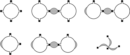
Figure 18: Graphical representation of the fourth cumulant. The notation is explained in LeDoussalWiesePREPg . Each diagram corresponds to a square bracket in Eq. (C.21), in the same order.

From (C.5) one has:

$$\sum_{e}\tilde{S}^{\prime}_{1,abe} = \sum_{e}\frac{\tilde{B}^{\prime\prime}_{ab}}{1+4I_{2}\tilde{B}^{\prime\prime}_{ab}}Y_{abe}$$ (C.16)

$$\frac{1}{2}\sum_{ef}Q^{\prime}_{1abef} = \sum_{ef}\Big{[}\frac{\tilde{B}^{\prime\prime}_{ab}}{1+4I_{2}\tilde{B}^{\prime\prime}_{ab}}Z_{abef}+\frac{\tilde{B}^{\prime\prime\prime}_{ab}}{2(1+4I_{2}\tilde{B}^{\prime\prime}_{ab})^{3}}Y_{abe}Y_{abf}\Big{]}\ ,\qquad$$ (C.17)

where we have used $B^{\prime\prime\prime}(\tilde{\chi}^{(0)}_{ab})=\tilde{B}^{\prime\prime\prime}_{ab}/((1+4I_{2}\tilde{B}^{\prime\prime}_{ab})^{3}$ obtained by further differentiation of (4.29) with respect to $v_{ab}^{2}$. We also define

$$Y_{abe}=T\tilde{\chi}^{(1)}_{ab} = 4I_{2}\Big{[}-\frac{1}{2}(\tilde{S}^{\prime}_{1,aae}+\tilde{S}^{\prime}_{1,bbe})+\tilde{S}^{\prime}_{1,abe}\Big{]}+2I_{2}T(\tilde{B}^{\prime}_{ae}+\tilde{B}^{\prime}_{be})$$ (C.18)

$$+8I_{3}\Big{[}-\frac{1}{2}(\tilde{B}^{\prime}_{aa}+\tilde{B}^{\prime}_{bb})(\tilde{B}^{\prime}_{ae}+\tilde{B}^{\prime}_{be})+\frac{1}{2}(\tilde{B}^{\prime}_{ae}\tilde{B}^{\prime}_{ae}+\tilde{B}^{\prime}_{be}\tilde{B}^{\prime}_{be})+\tilde{B}^{\prime}_{ab}(\tilde{B}^{\prime}_{ae}+\tilde{B}^{\prime}_{be})-\tilde{B}^{\prime}_{ae}\tilde{B}^{\prime}_{be}\Big{]}\ ,\qquad$$

and

$$Z_{abef} = T^{2}\tilde{\chi}^{(2)}_{ab}=2I_{2}\Big{[}\tilde{Q}^{\prime}_{1,abef}-\frac{1}{2}\tilde{Q}^{\prime}_{1,aaef}-\frac{1}{2}\tilde{Q}^{\prime}_{1,bbef}\Big{]}+2I_{2}T(\tilde{S}^{\prime}_{1,aef}+\tilde{S}^{\prime}_{1,bef})+4I_{3}T(\tilde{B}^{\prime}_{ae}\tilde{B}^{\prime}_{af}+\tilde{B}^{\prime}_{be}\tilde{B}^{\prime}_{bf})$$

$$+8I_{3}\Big{[}-(\tilde{B}^{\prime}_{aa}\tilde{S}^{\prime}_{1,aef}+\tilde{B}^{\prime}_{bb}\tilde{S}^{\prime}_{1,bef})-(\tilde{B}^{\prime}_{ae}\tilde{S}^{\prime}_{1,aaf}+\tilde{B}^{\prime}_{be}\tilde{S}^{\prime}_{1,bbf})+(\tilde{B}^{\prime}_{af}\tilde{S}^{\prime}_{1,fae}+\tilde{B}^{\prime}_{bf}\tilde{S}^{\prime}_{1,fbe})$$

$$\qquad\quad+\tilde{B}^{\prime}_{ab}(\tilde{S}^{\prime}_{1,bef}+\tilde{S}^{\prime}_{1,aef})+(\tilde{B}^{\prime}_{ae}\tilde{S}^{\prime}_{1,abf}+\tilde{B}^{\prime}_{be}\tilde{S}^{\prime}_{1,abf})-(\tilde{B}^{\prime}_{af}\tilde{S}^{\prime}_{1,fbe}+\tilde{B}^{\prime}_{bf}\tilde{S}^{\prime}_{1,fae})\Big{]}$$

$$+8I_{4}\Big{[}\tilde{B}^{\prime}_{ae}\tilde{B}^{\prime}_{ae}(2\tilde{B}^{\prime}_{af}+\tilde{B}^{\prime}_{ef})+\tilde{B}^{\prime}_{be}\tilde{B}^{\prime}_{be}(2\tilde{B}^{\prime}_{bf}+\tilde{B}^{\prime}_{ef})-(\tilde{B}^{\prime}_{ae}\tilde{B}^{\prime}_{af}+\tilde{B}^{\prime}_{be}\tilde{B}^{\prime}_{bf})\tilde{B}^{\prime}_{ef}-3\tilde{B}^{\prime}_{aa}(\tilde{B}^{\prime}_{af}\tilde{B}^{\prime}_{ae}+\tilde{B}^{\prime}_{bf}\tilde{B}^{\prime}_{be})$$

$$\qquad\quad-2\tilde{B}^{\prime}_{ae}\tilde{B}^{\prime}_{be}(\tilde{B}^{\prime}_{af}+\tilde{B}^{\prime}_{bf}+\tilde{B}^{\prime}_{ef})+2\tilde{B}^{\prime}_{ae}\tilde{B}^{\prime}_{bf}\tilde{B}^{\prime}_{ef}+2\tilde{B}^{\prime}_{ab}(\tilde{B}^{\prime}_{af}\tilde{B}^{\prime}_{ae}+\tilde{B}^{\prime}_{bf}\tilde{B}^{\prime}_{be}+\tilde{B}^{\prime}_{ae}\tilde{B}^{\prime}_{bf})\Big{]}\ ,$$

which should be further symmetrized over $e,f$ for later use (indicated by $\text{sym}_{ef}$ below).

The fourth cumulant equation yields, regrouping and simplifying the denominators (and using also the third cumulant equation):

$$\frac{1}{2}\tilde{Q}^{\prime}_{1abef}+2I_{2}\tilde{B}^{\prime\prime}_{ab}(\frac{1}{2}\tilde{Q}^{\prime}_{1aaef}+\frac{1}{2}\tilde{Q}^{\prime}_{1bbef})=\frac{1}{2}\tilde{B}^{\prime\prime\prime}_{ab}\frac{\tilde{S}^{\prime}_{1,abe}}{\tilde{B}^{\prime\prime}_{ab}}\frac{\tilde{S}^{\prime}_{1,abf}}{\tilde{B}^{\prime\prime}_{ab}}+2I_{2}T\text{sym}_{ef}[\tilde{B}^{\prime\prime}_{ab}(\tilde{S}^{\prime}_{1,aef}+\tilde{S}^{\prime}_{1,bef})]$$

$$+4I_{3}T\tilde{B}^{\prime\prime}_{ab}(\tilde{B}^{\prime}_{ae}\tilde{B}^{\prime}_{af}+\tilde{B}^{\prime}_{be}\tilde{B}^{\prime}_{bf})+8I_{3}\tilde{B}^{\prime\prime}_{ab}\text{sym}_{ef}\Big{[}-(\tilde{B}^{\prime}_{aa}\tilde{S}^{\prime}_{1,aef}+\tilde{B}^{\prime}_{bb}\tilde{S}^{\prime}_{1,bef})-(\tilde{B}^{\prime}_{ae}\tilde{S}^{\prime}_{1,aaf}+\tilde{B}^{\prime}_{be}\tilde{S}^{\prime}_{1,bbf})$$

$$+(\tilde{B}^{\prime}_{af}\tilde{S}^{\prime}_{1,fae}+\tilde{B}^{\prime}_{bf}\tilde{S}^{\prime}_{1,fbe})+\tilde{B}^{\prime}_{ab}(\tilde{S}^{\prime}_{1,bef}+\tilde{S}^{\prime}_{1,aef})+(\tilde{B}^{\prime}_{ae}\tilde{S}^{\prime}_{1,abf}+\tilde{B}^{\prime}_{be}\tilde{S}^{\prime}_{1,abf})-(\tilde{B}^{\prime}_{af}\tilde{S}^{\prime}_{1,fbe}+\tilde{B}^{\prime}_{bf}\tilde{S}^{\prime}_{1,fae})\Big{]}$$

$$+8I_{4}\tilde{B}^{\prime\prime}_{ab}\text{sym}_{ef}\Big{[}\tilde{B}^{\prime}_{ae}\tilde{B}^{\prime}_{ae}(2\tilde{B}^{\prime}_{af}+\tilde{B}^{\prime}_{ef})+\tilde{B}^{\prime}_{be}\tilde{B}^{\prime}_{be}(2\tilde{B}^{\prime}_{bf}+\tilde{B}^{\prime}_{ef})-(\tilde{B}^{\prime}_{ae}\tilde{B}^{\prime}_{af}+\tilde{B}^{\prime}_{be}\tilde{B}^{\prime}_{bf})\tilde{B}^{\prime}_{ef}-3\tilde{B}^{\prime}_{aa}(\tilde{B}^{\prime}_{af}\tilde{B}^{\prime}_{ae}+\tilde{B}^{\prime}_{bf}\tilde{B}^{\prime}_{be})$$

$$-2\tilde{B}^{\prime}_{ae}\tilde{B}^{\prime}_{be}(\tilde{B}^{\prime}_{af}+\tilde{B}^{\prime}_{bf}+\tilde{B}^{\prime}_{ef})+2\tilde{B}^{\prime}_{ae}\tilde{B}^{\prime}_{bf}\tilde{B}^{\prime}_{ef}+2\tilde{B}^{\prime}_{ab}(\tilde{B}^{\prime}_{af}\tilde{B}^{\prime}_{ae}+\tilde{B}^{\prime}_{bf}\tilde{B}^{\prime}_{be}+\tilde{B}^{\prime}_{ae}\tilde{B}^{\prime}_{bf})\Big{]}.$$ (C.19)

Setting $a=b$ and solving one finds:

$$\frac{1}{2}\tilde{Q}^{\prime}_{aaef}=\frac{4I_{2}T\tilde{B}^{\prime\prime}(0)}{1+4I_{2}\tilde{B}^{\prime\prime}(0)}\text{sym}_{ef}\tilde{S}^{\prime}_{1,aef}+\left[\frac{8T^{2}I_{2}^{2}\tilde{B}^{\prime\prime\prime}(0)}{(1+4I_{2}\tilde{B}^{\prime\prime}(0))^{3}}+\frac{8I_{3}\tilde{B}^{\prime\prime}(0)T}{1+4I_{2}\tilde{B}^{\prime\prime}(0)}\right]\tilde{B}^{\prime}_{ae}\tilde{B}^{\prime}_{af}$$ (C.20)

This gives the final result for the fourth cumulant:

$$Q_{abcd} = \mbox{Sym}_{abcd}\bigg{\{}$$

$$48\!\! \Big{[} \!-4\tilde{B}^{\prime}_{0}\tilde{B}^{\prime}_{ab}\tilde{B}^{\prime}_{ac}\tilde{B}^{\prime}_{ad}+4(\tilde{B}^{\prime}_{ab})^{2}\tilde{B}^{\prime}_{ac}\tilde{B}^{\prime}_{ad}+2(\tilde{B}^{\prime}_{ab})^{2}\tilde{B}^{\prime}_{ad}\tilde{B}^{\prime}_{bc}-4\tilde{B}^{\prime}_{ab}\tilde{B}^{\prime}_{ac}\tilde{B}^{\prime}_{ad}\tilde{B}^{\prime}_{bc}+\tilde{B}^{\prime}_{ab}\tilde{B}^{\prime}_{ad}\tilde{B}^{\prime}_{bc}\tilde{B}^{\prime}_{cd}\Big{]}I_{4}$$

$$+192\!\! \Big{[} \!4(\tilde{B}^{\prime}_{0})^{2}\tilde{B}^{\prime}_{ab}\tilde{B}^{\prime}_{cd}{\tilde{B}^{\prime\prime}}_{ac}-4\tilde{B}^{\prime}_{0}(\tilde{B}^{\prime}_{ab})^{2}\tilde{B}^{\prime}_{cd}{\tilde{B}^{\prime\prime}}_{ac}-8\tilde{B}^{\prime}_{0}\tilde{B}^{\prime}_{ab}\tilde{B}^{\prime}_{ac}\tilde{B}^{\prime}_{cd}{\tilde{B}^{\prime\prime}}_{ac}+4(\tilde{B}^{\prime}_{ab})^{2}\tilde{B}^{\prime}_{ac}\tilde{B}^{\prime}_{cd}{\tilde{B}^{\prime\prime}}_{ac}+4\tilde{B}^{\prime}_{ab}(\tilde{B}^{\prime}_{ac})^{2}\tilde{B}^{\prime}_{cd}{\tilde{B}^{\prime\prime}}_{ac}$$

$$+8\tilde{B}^{\prime}_{0}\tilde{B}^{\prime}_{ab}\tilde{B}^{\prime}_{bc}\tilde{B}^{\prime}_{cd}{\tilde{B}^{\prime\prime}}_{ac}-8\tilde{B}^{\prime}_{0}\tilde{B}^{\prime}_{ac}\tilde{B}^{\prime}_{bc}\tilde{B}^{\prime}_{cd}{\tilde{B}^{\prime\prime}}_{ac}-8\tilde{B}^{\prime}_{ab}\tilde{B}^{\prime}_{ac}\tilde{B}^{\prime}_{bc}\tilde{B}^{\prime}_{cd}{\tilde{B}^{\prime\prime}}_{ac}+4(\tilde{B}^{\prime}_{ac})^{2}\tilde{B}^{\prime}_{bc}\tilde{B}^{\prime}_{cd}{\tilde{B}^{\prime\prime}}_{ac}+4(\tilde{B}^{\prime}_{ab})^{2}\tilde{B}^{\prime}_{ac}\tilde{B}^{\prime}_{ad}{\tilde{B}^{\prime\prime}}_{ad}$$

$$-4(\tilde{B}^{\prime}_{ab})^{2}\tilde{B}^{\prime}_{ac}\tilde{B}^{\prime}_{cd}{\tilde{B}^{\prime\prime}}_{ad}+2\tilde{B}^{\prime}_{ab}\tilde{B}^{\prime}_{ac}\tilde{B}^{\prime}_{bd}\tilde{B}^{\prime}_{cd}{\tilde{B}^{\prime\prime}}_{ad}+(\tilde{B}^{\prime}_{ab})^{2}(\tilde{B}^{\prime}_{cd})^{2}{\tilde{B}^{\prime\prime}}_{ad}+4(\tilde{B}^{\prime}_{0})^{2}\tilde{B}^{\prime}_{ac}\tilde{B}^{\prime}_{cd}{\tilde{B}^{\prime\prime}}_{bc}-4\tilde{B}^{\prime}_{0}(\tilde{B}^{\prime}_{ac})^{2}\tilde{B}^{\prime}_{cd}{\tilde{B}^{\prime\prime}}_{bc}$$

$$+(\tilde{B}^{\prime}_{ad})^{2}(\tilde{B}^{\prime}_{cd})^{2}{\tilde{B}^{\prime\prime}}_{bd}\Big{]}I_{3}^{2}$$

$$+192T\!\! \Big{[} \!2\tilde{B}^{\prime}_{ab}\tilde{B}^{\prime}_{ac}\tilde{B}^{\prime}_{ad}\tilde{B}^{\prime\prime}_{ab}+2\tilde{B}^{\prime}_{ab}\tilde{B}^{\prime}_{ad}\tilde{B}^{\prime}_{bc}\tilde{B}^{\prime\prime}_{ab}-2\tilde{B}^{\prime}_{0}\tilde{B}^{\prime}_{ab}\tilde{B}^{\prime}_{ad}\tilde{B}^{\prime\prime}_{ac}+(\tilde{B}^{\prime}_{ab})^{2}\tilde{B}^{\prime}_{ad}\tilde{B}^{\prime\prime}_{ac}-2\tilde{B}^{\prime}_{ab}\tilde{B}^{\prime}_{ad}\tilde{B}^{\prime}_{bc}\tilde{B}^{\prime\prime}_{ac}-2\tilde{B}^{\prime}_{0}\tilde{B}^{\prime}_{ab}\tilde{B}^{\prime}_{cd}\tilde{B}^{\prime\prime}_{ac}$$

$$+(\tilde{B}^{\prime}_{ab})^{2}\tilde{B}^{\prime}_{cd}\tilde{B}^{\prime\prime}_{ac}-2\tilde{B}^{\prime}_{ab}\tilde{B}^{\prime}_{ac}\tilde{B}^{\prime}_{ad}\tilde{B}^{\prime\prime}_{0}\Big{]}\frac{I_{2}I_{3}}{1+4I_{2}\tilde{B}^{\prime\prime}_{0}}$$

$$+32T\!\! \Big{[}\! \tilde{B}^{\prime}_{ab}\tilde{B}^{\prime}_{ac}\tilde{B}^{\prime}_{ad}\Big{]}\frac{I_{3}}{1+4I_{2}\tilde{B}^{\prime\prime}_{0}}$$

$$+48T^{2}\!\! \Big{[} \!\tilde{B}^{\prime}_{ab}\tilde{B}^{\prime}_{ad}\tilde{B}^{\prime\prime}_{ac}+\tilde{B}^{\prime}_{ab}\tilde{B}^{\prime}_{cd}\tilde{B}^{\prime\prime}_{ac}\Big{]}\frac{I_{2}^{2}}{(1+4I_{2}\tilde{B}^{\prime\prime}_{0})^{2}}$$

$$-128T^{2}\!\! \Big{[} \!\tilde{B}^{\prime}_{ac}\tilde{B}^{\prime}_{bc}\tilde{B}^{\prime}_{cd}\tilde{B}^{\prime\prime\prime}_{0}\Big{]}\frac{I_{2}^{3}}{(1+4I_{2}\tilde{B}^{\prime\prime}_{0})^{3}}\bigg{\}}$$ (C.21)

where $\mathrm{Sym}_{abcd}$ denotes $1/24$ times the sum of all 24 permutations of the indices $a,b,c,d$, and we note $\tilde{B}^{\prime}_{0}=\tilde{B}^{\prime}(0)$, $\tilde{B}^{\prime\prime}_{0}=\tilde{B}^{\prime\prime}(0)$ and $\tilde{B}^{\prime\prime\prime}_{0}=\tilde{B}^{\prime\prime\prime}(0)$. Note that all terms containing $\tilde{B}^{\prime}(0)$ can be eliminated by the redefinition $\tilde{B}^{\prime}_{\mathrm{new}}(x)=\tilde{B}^{\prime}(x)-\tilde{B}^{\prime}(0)$.

Appendix D Cumulant expansion for non-local effective action

The cumulant expansion can be generalized to study the effective action for non-uniform configurations. The functional $\tilde{U}[v\cdot v]$ is a functional of the field $v_{ab}^{2}(x)$ and can be expanded as:

$$\tilde{U}[vv]=\frac{-1}{2T^{2}}\sum_{ab}\tilde{B}[v_{ab}^{2}]-\frac{1}{3!T^{3}}\sum_{abc}\tilde{S}[v_{ab}^{2},v_{bc}^{2},v_{ca}^{2}]+\dots\ .$$ (D.1)

The self-consistent equation (3.31) then yields, by a similar expansion in numbers of sums:

$$\frac{\delta\tilde{B}[v\cdot v]}{\delta(v_{a}(x)\cdot v_{b}(x))}=B^{\prime}\bigg{(}v_{ab}^{2}(x)+2TI_{1}$$

$$\qquad\quad~{}+4\int_{y}C_{xy}^{2}\Big{[}\frac{\delta\tilde{B}[v\cdot v]}{\delta(v_{a}(y)\cdot v_{b}(y))}-\frac{\delta\tilde{B}[v\cdot v]}{\delta(v_{a}(y)\cdot v_{a}(y))}\Big{]}\bigg{)}$$ (D.2)

Appendix E Analysis for all $m$ and short range case

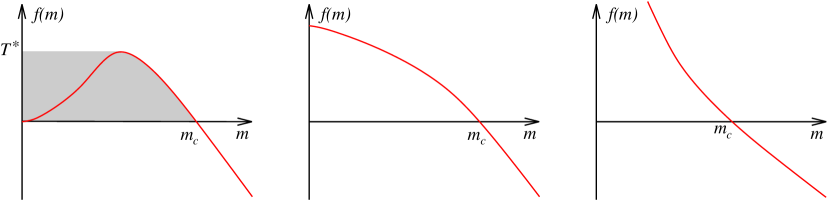
      $\theta(\gamma)>0$ $\theta(\gamma)=0$ $\theta(\gamma)<0$

Figure 20: The function $f(m)$ defined in Eq. (E.2).

To refine the analysis and study the behavior for all values of $m$, let us rewrite from (6.10) the condition that $\tilde{B}$ remains analytic for all $m$. It reads:

$$T>f(m)\qquad\text{for all}\quad m$$ (E.1)

$$f(m)=\frac{(B^{\prime\prime})^{-1}\left(\frac{1}{4I_{2}}\right)}{2I_{1}}=\frac{(4g\gamma I_{2})^{\frac{1}{1+\gamma}}-a^{2}}{2I_{1}}\ ,$$ (E.2)

where we have also inserted the value of the inverse function, with $B^{\prime\prime}((B^{\prime\prime})^{-1}(x))=x$, for the power law models. This condition is equivalent to the vanishing of the replicon, i.e. it is the line where the RS solution of the GVM becomes unstable to RSB.

One can then plot (see Fig. 20) the function $f(m)$ for the three cases defined in the text, LR $\theta(\gamma)>0$, marginal $\theta(\gamma)=0$ and SR $\theta(\gamma)<0$ where $\theta(\gamma)=d-2+\frac{4-d}{1+\gamma}$. The LR and marginal cases, which correspond to continuous and one step marginal RSB solutions, have been discussed in the text and there the FRG gives back exactly $\sigma_{m}(0)$ of the MP solution. We defer the detailed study of the SR case to further work, and give here a few general remarks.

First one notices on Fig. 20 that solving the FRG equation decreasing the mass from infinity one first has the analytic solution which coincides with the RS one. For $T>T^{*}=\max_{m}f(m)$ it remains analytic down to $m=0$. For $T<T^{*}$ a cusp arises when the left branch of the line is reached. Thus despite the reentrance of the analytic solution at small $m$, freezing of the FRG solution has already occurred and it is clearly important to understand how to extend the FRG in the shaded region. On the other hand, a 1-step solution of the MP saddle point equations exists, obtained by varying the free energy w.r.t. $u_{c}$. Its precise boundary depends on the model, but it is generally contained within the shaded region (for details see MezardParisi1991 ; Goldschmidt1993 ; Engel1993 ; CugliandoloLeDoussal1996b ). An intriguing property of the GVM is the simultaneous existence, within the rightmost portion of the shaded region near the axis $m=0$, of two locally stable solutions, one RS and the other 1-step RSB. Thus, although the line in Fig. 20 is the locus of a continuous transition from RS to RSB, in this rightmost portion of the $m-T$ diagram, the 1-step non-marginal RSB solution appears discontinuously, before the line is reached as $T$ is lowered. Work is in progress to make contact between FRG and RSB in this SR case, and in particular to understand whether there are also two branches of solutions of the FRG equation in that region.

Appendix F Finite-temperature fixed points

From the RG point of view it is interesting to search for finite temperature fixed points (FP) of the FRG equation, especially in view of future extensions to finite $N$ (since we know at least in some cases, that these persist at finite $N$). It is convenient to use Eq. (7.8). These FPs exist only in the marginal case $\theta=0$, i.e. $\zeta=(2-d)/2$ for $d<2$ or $\zeta=0$ for $d=2$, so that $T_{m}=4A_{d}T/\epsilon$ does not flow. This is the case studied here.

F.1 $d<2$

Following the same steps as in Section VII.2, the general solution of the fixed-point condition $m\partial_{m}x(y)=0$ in (7.8) for a fixed value of $\zeta>0$, imposing $x(y_{0})=0$ is

$$x^{*}(y) = \frac{y}{\epsilon}-\frac{y_{0}}{2\zeta}+\frac{\epsilon-2\zeta}{2\zeta\epsilon}\,y_{0}\left(\frac{y_{0}}{y}\right)^{\frac{2\zeta}{\epsilon-2\zeta}}$$ (F.1)

$$+\frac{T_{m}\epsilon x^{\prime}_{0}}{2\zeta(\epsilon x^{\prime}_{0}-1)}\left[\left(\frac{y_{0}}{y}\right)^{\frac{2\zeta}{\epsilon-2\zeta}}-1\right]\ .$$

Taking a derivative at $y=y_{0}$, we obtain a self-consistency condition for $x^{\prime}_{0}$. One solution is $x^{\prime}_{0}=0$, the “zero-temperature” fixed point discussed in Section VII.2. The other one is

$$-\epsilon x^{\prime}_{0}=\frac{\epsilon T_{m}}{y_{0}(\epsilon-2\zeta)}-1\ ,$$ (F.2)

with the condition that it must be positive. Reinserting in (F.1) we obtain the final form for the finite-temperature fixed point:

$$x^{*}(y) = \frac{y}{\epsilon}-\frac{y_{0}}{2\zeta}+\frac{\epsilon-2\zeta}{2\zeta\epsilon}\,y_{0}\left(\frac{y_{0}}{y}\right)^{\!\frac{2\zeta}{\epsilon-2\zeta}}$$ (F.3)

$$+\frac{1}{2\zeta}\left[T_{m}-\frac{y_{0}(\epsilon-2\zeta)}{\epsilon}\right]\left[\left(\frac{y_{0}}{y}\right)^{\!\frac{2\zeta}{\epsilon-2\zeta}}-1\right]\qquad$$

$$= \frac{y-y_{0}}{\epsilon}+\frac{T_{m}}{2\zeta}\left[\left(\frac{y_{0}}{y}\right)^{\!\frac{2\zeta}{\epsilon-2\zeta}}-1\right]$$

The term in the second line of (F.3) was not present in the “zero-temperature” fixed-point solution (7.15). Note that it does not vanish at $T=0$ but at the higher temperature $T=T_{c}$ such that $T_{m}=\frac{y_{0}(\epsilon-2\zeta)}{\epsilon}$. At this point, also $x^{\prime}_{0}$ vanishes and the solution $b^{\prime}(x)=-y(x)$ becomes non-analytic. The fixed-point analysis alone does neither fix the value of $y_{0}$, nor $T_{c}$.

However we can now explicitly check that this fixed-point solution identifies with the analytic solution (7.27), (7.28) when setting $m\to 0$, using $\tilde{T}_{m}=T_{m}/(2-d)$ and $\zeta=1/\gamma=(2-d)/2$. This identification works only for $T>T_{c}$, and since $y_{0}$ is now fixed by (7.28), we can compute $T_{c}$ and find that it is given by (7.39). Below $T_{c}$ the solution freezes at $m=m_{c}$ at the zero temperature fixed point.

F.2 $d=2$

Let us now solve the fixed point condition $m\partial_{m}x(y)=0$ in (7.8) for $\zeta=0$, imposing $x(y_{0})=0$. One finds:

$$x^{*}(y)=\frac{y-y_{0}}{\epsilon}-\left(\frac{y_{0}}{\epsilon}+\frac{T_{m}x^{\prime}_{0}}{\epsilon x^{\prime}_{0}-1}\right)\ln(y/y_{0})\ .$$ (F.4)

Determining $x^{\prime}_{0}$ again one finds, in addition to the solution $x^{\prime}_{0}=0$

$$-\epsilon x^{\prime}_{0}=\frac{T_{m}}{y_{0}}-1\ .$$ (F.5)

Reinserting one finds finally the finite-temperature fixed points

$$x^{*}(y)=\frac{y-y_{0}}{\epsilon}-\frac{T}{\epsilon\pi}\ln(y/y_{0})\ ,$$ (F.6)

with $\epsilon=2$ and $T_{m}=T/\pi$. There is thus a line of fixed points with $\zeta=0$ in $d=2$, parameterized by temperature, $y_{0}$ being again undetermined.

To compare with the solution of the flow equation, we obviously need to consider a broader class of SR models with $B^{\prime}(z)=-g\exp(-z/a^{2})$. The solution is then:

$$x = a^{2}\ln(y_{0}/y)+{\epsilon}^{{-1}}(y-y_{0})$$ (F.7)

$$y_{0} = \tilde{g}m^{T/(\pi a^{2})-\epsilon}\Lambda^{-T/(\pi a^{2})}$$ (F.8)

with $\epsilon=2$. For small disorder $\tilde{g}$, and $T>T_{c}=\epsilon\pi a^{2}=2\pi a^{2}$, $y_{0}(m)$ flows to zero as $m\to 0$ and the solution remains analytic. For $T<T_{c}$ the solution develops a cusp when $y_{0}$ reaches $y_{0}=y_{0}(m_{c})=\epsilon a^{2}$, i.e. at the Larkin mass:

$$m_{c}=(\tilde{g}/a^{2}\epsilon)^{\frac{1}{2(1-T/T_{c})}}\Lambda^{\frac{T}{T_{c}-T}}\ .$$ (F.9)

Thus only for $T=T_{c}$ the solution reaches for $m\to 0$ an analytic finite-$T$ fixed point associated with $\zeta=0$, of the form (F.6). Thus in $d=2$ the line of finite-temperature fixed points with $\zeta=0$ corresponds to the line of critical fixed points as the parameter $a$ is varied.

Appendix G RG formulation of the RSB solution

In this appendix, we derive simple RG equations for the MP solution in the full RSB case. This gives a more direct derivation of the key-equations (8.51) and (8.52). We start from (see (8.4) and (8.5), equivalent to (5.4) of MP):

$$\sigma(u)=-\frac{2}{T}B^{\prime}\left(2T\int_{k}(\tilde{G}(k)-G(k,u))\right)\ .$$ (G.1)

Taking a derivative with respect to $u$ yields

$$1=4B^{\prime\prime}\left(2T\int_{k}\tilde{G}(k)-G(k,u)\right)\int_{k}\frac{1}{(k^{2}+\mu+[\sigma](u))^{2}}$$ (G.2)

for all $u$ such that $\sigma^{\prime}(u)\neq 0$. Using that due to (see (8.5), equivalent to (5.2) of MP):

$$\tilde{G}(k)-G(k,u) = \frac{1}{u(k^{2}+{m^{2}}+[\sigma](u))}$$ (G.3)

$$-\int_{u}^{1}\frac{{\mathrm{d}}v}{v^{2}}\frac{1}{k^{2}+{m^{2}}+[\sigma](v)}$$

we have

$$\partial_{u}(\tilde{G}(k)-G(k,u))=-\frac{\sigma^{\prime}(u)}{(k^{2}+{m^{2}}+[\sigma](u))^{2}}\ .$$ (G.4)

On the other hand, we can take a derivative of (G.1) with respect to ${m^{2}}$:

$$\partial_{m^{2}}\sigma(u) = -4B^{\prime\prime}\left(2T\int_{k}(\tilde{G}(k)-G(k,u))\right)$$ (G.5)

$$\times\int_{k}\partial_{m^{2}}(\tilde{G}(k)-G(k,u))\ .$$

Eliminating $B^{\prime\prime}(\dots)$ one finds:

$$\partial_{m^{2}}\sigma(u)\int_{k}\frac{1}{(k^{2}+{m^{2}}+[\sigma](u))^{2}}$$

$$\qquad=-\int_{k}\partial_{m^{2}}(\tilde{G}(k)-G(k,u))\ .\qquad$$ (G.6)

Taking another derivative with respect to $u$ after using (G.4) gives

$$\partial_{u}\!\int_{k}\frac{\partial_{{m^{2}}}\sigma(u)}{(k^{2}+{m^{2}}+[\sigma](u))^{2}}=\partial_{{m^{2}}}\!\int_{k}\frac{\sigma^{\prime}(u)}{(k^{2}+{m^{2}}+[\sigma](u))^{2}}\ .$$ (G.7)

Noting that the derivatives of the numerator cancel, we get

$$\int_{k}\frac{u\sigma^{\prime}(u)\partial_{{m^{2}}}\sigma(u)}{(k^{2}+{m^{2}}+[\sigma](u))^{3}}=\int_{k}\frac{\sigma^{\prime}(u)(1+\partial_{{m^{2}}}[\sigma](u))}{(k^{2}+{m^{2}}+[\sigma](u))^{3}}\ .$$ (G.8)

Since for all $u$, $\int_{k}{(k^{2}+{m^{2}}+[\sigma](u))^{-3}}\neq 0$ and by assumption $\sigma^{\prime}(u)\neq 0$, RSB reveals its universality in the simple relation:

$$u\partial_{m^{2}}\sigma(u)=1+\partial_{m^{2}}[\sigma](u)\ ,$$ (G.9)

which, upon another derivation, yields the two “RG equations”:

$${m^{2}}\frac{{\mathrm{d}}}{{\mathrm{d}}{m^{2}}}\left({m^{2}}+[\sigma](u)\right) = 0$$ (G.10)

$${m^{2}}\frac{{\mathrm{d}}}{{\mathrm{d}}{m^{2}}}\sigma(u) = 0\ .$$ (G.11)

Appendix H Convergence to the fixed point

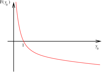
Figure 22: The function (H.5), describing the approach to the fixed point in presence of an additional bare power law tail.

Since we have found the solution of the FRG equation for arbitrary disorder correlations, it is instructive to study the convergence to the FRG fixed point in the case where the inital disorder is not of the simple form (2.10) on an explicit example. We start from a disorder correlator which is the superposition of two power laws:

$$-B^{\prime}(z)=\frac{g}{(a^{2}+z)^{\gamma}}+C^{\prime}\frac{g}{(a^{2}+z)^{\alpha}}$$ (H.1)

with $\alpha>\gamma$, s.t. for large $z$ the first term dominates and fixes the exponent $\zeta=\frac{\epsilon}{2(1+\gamma)}$. We will determine the inverse function $\Phi(x)$ only for $C^{\prime}$ small. One finds

$$-\frac{\epsilon}{4A_{d}}\,\Phi^{\prime}\!\left(\frac{y}{4Ad}\right)=y^{-\frac{1}{\gamma}-1}+Cy^{-\frac{1}{\delta}-1}\ ,$$ (H.2)

with $C^{\prime}\sim C$, and we have defined

$$\frac{1}{\delta}=\frac{1-\alpha+\gamma}{\gamma}\ .$$ (H.3)

We have chosen $\tilde{g}=(\gamma/\epsilon)^{\gamma}$ to simplify all prefactors.

Inserting into (8.42), we obtain:

$$(y_{0}m^{\epsilon-2\zeta})^{-\frac{1}{\gamma}-1}+C(y_{0}m^{\epsilon-2\zeta})^{-\frac{1}{\delta}-1}=m^{-\epsilon}\ .$$ (H.4)

By multiplying with $m^{\epsilon}$ and $y_{0}^{\frac{\delta+1}{\delta}}$, we obtain the equivalent formula

$${\mathrm{F}}(y_{0}):=y_{0}^{\frac{\gamma-\delta}{\gamma\delta}}-y_{0}^{\frac{\delta+1}{\delta}}=-Cm^{\frac{\delta-\gamma}{(1+\gamma)\delta}\epsilon}\ .$$ (H.5)

The left-hand side is plotted on figure 22; note that always the first exponent is negative, and the second and third are positive. Thus the solution for $m=0$ or $C=0$ is simply $y_{0}=1$. For non-vanishing $C$ and $m$, the solution can be obtained graphically as the intersection of ${\mathrm{F}}(y_{0})$ with $-Cm^{\frac{\delta-\gamma}{(1+\gamma)\delta}\epsilon}$. Note that there is a solution for any $C$.

For $m\to 0$, the approach to $y_{0}=1$ is obtained by linearizing $\mathrm{F}(y_{0})$, with the result

$$y_{0}-1\approx\frac{\gamma C}{1+\gamma}m^{\frac{\delta-\gamma}{(1+\gamma)\delta}\epsilon}\ .$$ (H.6)

Appendix I Pure $O(N)$ models, non-analytic effective action

In this Section we recall the corresponding result for the effective action of the generic pure $O(N)$ model at large $N$. One mechanism by which the effective action may becomes non-analytic is given on standard example of $\phi^{4}$.

I.1 Self-consistent equation

The generic $O(N)$ model in dimension $d$ is defined by the action:

$$S=\frac{1}{T}\int_{x}\left[\frac{1}{2}\left(\nabla u(x)\right)^{2}+\frac{1}{2}m^{2}u(x)^{2}+NV\Big{(}\frac{u(x)^{2}}{N}\Big{)}\right]$$ (I.1)

Here $m$ is used as a parameter, the bare mass being $m_{b}^{2}=m^{2}+2V^{\prime}(0)$. For a uniform mode one has $\Gamma[u]=L^{d}\tilde{\Gamma}[v]$ in terms of the rescaled field $v=u/\sqrt{N}$. One defines:

$$\tilde{\Gamma}[v]=\frac{1}{2}m^{2}v^{2}+\tilde{V}(v^{2})=\tilde{W}(v^{2})\ .$$ (I.2)

Similarly, one defines

$$W(z)=\frac{1}{2}m^{2}z+V(z)\ ,$$ (I.3)

whether absorbing or not the mass into the (bare or renormalized) potential. Again, for $m=\infty$, one has $\tilde{V}=V$. The same method as in Section (III) yields the saddle point equations for infinite $N$:

$$\tilde{V}^{\prime}(v^{2}) = V^{\prime}(v^{2}+G(v))\qquad$$ (I.4)

$$G(v) = \int_{q}\frac{T}{q^{2}+m^{2}+2V^{\prime}(v^{2}+G(v))}\ .$$ (I.5)

More details, a graphical derivation, and the $1/N$ expansion are given in LeDoussalWiesePREPg . A condition for the stability of the theory is that:

$$2\tilde{W}^{\prime}(v^{2}):=m^{2}+2\tilde{V}^{\prime}(v^{2})\geq 0\quad\text{for all}\ v^{2}\ .$$ (I.6)

I.2 Solution and FRG equation

Let us start from the form

$$\tilde{W}^{\prime}(x)=W^{\prime}\left(x+T\int_{q}^{\Lambda}\frac{1}{q^{2}+2\tilde{W}^{\prime}(x)}\right)\ ,$$ (I.7)

The self-consistent solution of this equation is formally:

$$x = (W^{\prime})^{-1}\left(y\right)-T\int_{q}^{\Lambda}\frac{1}{q^{2}+2y}$$ (I.8)

$$y = \tilde{W}^{\prime}(x)\ .$$ (I.9)

and $y\geq 0$.

Let us write the associated FRG equation. One has

$$-m\partial_{m}\tilde{W}^{\prime}(x) = -m^{2}-2TW^{\prime\prime}\left(x+T\int_{q}^{\Lambda}\frac{1}{q^{2}+2\tilde{W}^{\prime}(x)}\right)$$

$$\times\left(-m\partial_{m}\tilde{W}^{\prime}(x)\right)\int_{q}^{\Lambda}\frac{1}{(q^{2}+2\tilde{W}^{\prime}(x))^{2}}$$

$$\tilde{W}^{\prime\prime}(x) = W^{\prime\prime}\left(x+T\int_{q}^{\Lambda}\frac{1}{q^{2}+2\tilde{W}^{\prime}(x)}\right)$$

$$\times\left(1-2T\tilde{W}^{\prime\prime}(x)\int_{q}^{\Lambda}\frac{1}{(q^{2}+2\tilde{W}^{\prime}(x))^{2}}\right)\ .$$

Thus:

$$-m\partial_{m}\tilde{W}^{\prime}(x)=2Tm^{2}\tilde{W}^{\prime\prime}(x)\int_{q}^{\Lambda}\frac{1}{(q^{2}+2\tilde{W}^{\prime}(x))^{2}}-m^{2}\ .$$ (I.12)

For $d<4$ taking $\Lambda$ to infinity, this becomes

$$-m\partial_{m}\tilde{W}^{\prime}(x)=2T\frac{A_{d}}{\epsilon}m^{2}\tilde{W}^{\prime\prime}(x)(2\tilde{W}^{\prime}(x))^{-\epsilon/2}-m^{2}\ .$$ (I.13)

I.3 $\phi^{4}$-theory and non-analytic behavior

For the $\phi^{4}$ theory $V(x)=\frac{g}{4}(x-1)^{2}$ this reads:

$$\tilde{W}^{\prime}(x) = \frac{1}{2}m^{2}+\frac{g}{2}(x-1)+\frac{gT}{2}\int_{q}^{\Lambda}\frac{1}{q^{2}+2\tilde{W}^{\prime}(x)}\qquad\quad$$ (I.14)

$$x(y) = \frac{2}{g}y+1-\frac{m^{2}}{g}-T\int_{q}^{\Lambda}\frac{1}{q^{2}+2y}$$ (I.15)

for $y\geq y_{0}$ with $x(y_{0})=0$. At $T=0$, as $m$ is decreased, there is a transition in any $d$ when $m_{b}^{2}=m^{2}-g$ vanishes. For $d>2$, the transition persists for $T<T_{c}$, and occurs when $m^{2}-g+gT\int_{q}^{\Lambda}\frac{1}{q^{2}}$ vanishes, with the standard result:

$$T_{c}\int_{q}^{\Lambda}\frac{1}{q^{2}}=1\ ,$$ (I.16)

which depends strongly on the UV-cutoff $\Lambda$. $y_{0}$ vanishes at the transition, and in the ordered phase the effective action has a non-analytic form. In addition of the branch (I.15) for $y\geq 0$, $x>x_{c}=1-\frac{m^{2}}{g}-T\int_{q}^{\Lambda}\frac{1}{q^{2}}$, the function $x(y)$ has a branch $y=0$ for $0<x<x_{c}$, where $x_{c}$ is the order parameter.

Exactly at $T=T_{c}$ we should recover that the effective action exhibits the standard power-law non-analyticity $\Gamma[M]=M^{1+\delta}$. Indeed, from the self-consistent solution (I.15), subtracting the same with $x=x_{c}$ and $y=0$ one gets

$$x(y)=\frac{2}{g}y+(2y)^{(d-2)/2}T_{c}\int_{k}^{\Lambda/2y}\frac{1}{k^{2}}\frac{1}{k^{2}+1}$$ (I.17)

for $2<d<4$. This corresponds to $\delta=(2+d)/(2-d)$. It can be recovered by solving the FRG equation. One can look for fixed-point solutions of the form

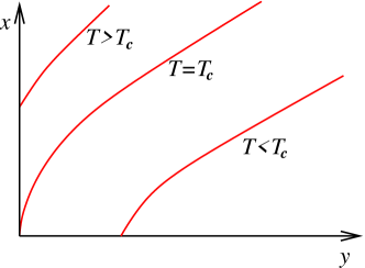
Figure 24: Relation between $x$ and $y$ in scalar field theory: above, at, and below the critical temperature.

$$\tilde{W}^{\prime}(x)=m^{\alpha}f(m^{\beta}x)\ .$$ (I.18)

If one wants the two first terms to dominate and to scale in the same way, one needs $\alpha\leq 2$ and $\beta=\alpha\epsilon/2-2$. For all three terms to scale the same way one needs $\alpha=2$, $\beta=2-d$. Inserting (I.18) into (I.13) yields

$$1-\alpha f(z)-\beta zf^{\prime}(z)=2T\frac{A_{d}}{\epsilon}f^{\prime}(z)(2f(z))^{-\epsilon/2}\ .$$ (I.19)

Again this can be transformed into a linear RG equation for $z(f)$:

$$(1-\alpha f)z^{\prime}(f)-\beta z(f)=2T\frac{A_{d}}{\epsilon}(2f)^{-\epsilon/2}\ .$$ (I.20)

The solutions of the above equation with $\alpha=2$, $\beta=2-d$ are:

$$z(f)=-2T\frac{A_{d}}{\epsilon}(2f-1)^{(d-2)/2}\int_{g}^{f}t^{-\epsilon/2}(2t-1)^{-d/2}$$ (I.21)

A particular solution is

$$z(f) = (2f-1)^{(d-2)/2}$$ (I.22)

$$\tilde{W}^{\prime}(x) = \frac{m^{2}}{2}+x^{2/(d-2)}\ .$$ (I.23)

In the limit of zero mass this yields $\tilde{V}^{\prime}(x)=x^{2/(d-2)}$.

One can also pursue the RG approach in the ordered phase, as is done usually in the form of a non-linear sigma model, and deal with a non-analytic effective action.

Although the mechanism for the disordered systems studied in the main text seems to be different from $\phi^{4}$-models, it raises the question of the meaning of the non-analyticity in the disordered problem. Is it the signature that we are dealing with a glass phase, where a symmetry has been broken? We know that for infinite $N$, this is also accompanied by RSB, but this does not have to be so in general, i.e. the cusp can arise without RSB, just from localization (single ground state dominance).

References

- (1) T. Nattermann, Theory of the random field Ising model, in A.P. Young, editor, Spin glasses and random fields, World Scientific, Singapore, 1997.
- (2) S. Lemerle, J. Ferré, C. Chappert, V. Mathet, T. Giamarchi and P. Le Doussal, Domain wall creep in an Ising ultrathin magnetic film, Phys. Rev. Lett. 80 (1998) 849.
- (3) A. Prevost, E. Rolley and C. Guthmann, Dynamics of a helium-4 meniscus on a strongly disordered cesium substrate, Phys. Rev. B 65 (2002) 064517/1–8.
- (4) D. Ertas and M. Kardar, Critical dynamics of contact line depinning, cond-mat/9401027 (1994).
- (5) G. Blatter, M.V. Feigel’man, V.B. Geshkenbein, A.I. Larkin and V.M. Vinokur, Vortices in high-temperature superconductors, Rev. Mod. Phys. 66 (1994) 1125.
- (6) T. Giamarchi and P. Le Doussal, Elastic theory of flux lattices in the presence of weak disorder, Phys. Rev. B 52 (1995) 1242–70.
- (7) T. Giamarchi and P. Le Doussal, Statics and dynamics of disordered elastic systems, in A.P. Young, editor, Spin glasses and random fields, World Scientific, Singapore, 1997, cond-mat/9705096.
- (8) T. Nattermann and S. Scheidl, Vortex-glass phases in type-ii superconductors, Advances in Physics 49 (2000) 607–704.
- (9) A.P. Young, Spin glasses and random fields. World Scientific, Singapore, 1997.
- (10) K.B. Efetov and A.I. Larkin, Sov. Phys. JETP 45 (1977) 1236.
- (11) A. Aharony, Y. Imry and S.K. Ma, Lowering of dimensionality in phase transitions with random fields, Phys. Rev. Lett. 37 (1976) 1364–7.
- (12) G. Grinstein, Ferromagnetic phase transitions in random fields: the breakdown of scaling laws, Phys. Rev. Lett. 37 (1976) 944–7.
- (13) G. Parisi and N. Sourlas, Random magnetic fields, supersymmetry, and negative dimensions, Phys. Rev. Lett. 43 (1979) 744–5.
- (14) J.L. Cardy, Nonperturbative effects in a scalar supersymmetric theory, Phys. Lett. 125 B (1983) 470–2.
- (15) M. Kardar, Replica Bethe ansatz studies of two-dimensional interfaces with quenched random impurities, Nucl. Phys. B 290 (1987) 582–602.
- (16) E. Brunet and B. Derrida, Ground state energy of a non-integer number of particles with delta attractive interactions, Physica A 279 (2000) 398–407.
- (17) E. Brunet and B. Derrida, Probability distribution of the free energy of a directed polymer in a random medium, Phys. Rev. E 61 (2000) 6789–801.
- (18) K. Johansson, math.PR/9910146.
- (19) M. Prähofer and H. Spohn, Statistical self-similarity of one-dimensional growth processes, Physica A 279 (2000) 342–52.
- (20) M. Lässig, On the renormalization of the Kardar-Parisi-Zhang equation, Nucl. Phys. B 448 (1995) 559–574.
- (21) K.J. Wiese, On the perturbation expansion of the KPZ-equation, J. Stat. Phys. 93 (1998) 143–154.
- (22) M. Lassig and H. Kinzelbach, Upper critical dimension of the Kardar-Parisi-Zhang equation, Phys. Rev. Lett. 78 (1997) 903–6.
- (23) E. Marinari, A. Pagnani and G. Parisi, Critical exponents of the KPZ equation via multi-surface coding numerical simulations, J. Phys. A 33 (2000) 8181–92.
- (24) M. Mézard and G. Parisi, Replica field theory for random manifolds, J. Phys. I (France) 1 (1991) 809–837.
- (25) L. Cugliandolo, J. Kurchan and P. Le Doussal, Large time off-equilibrium dynamics of a manifold in a random potential, Phys. Rev. Lett. 76 (1996) 2390.
- (26) L. Cugliandolo and P. Le Doussal, Large time off-equilibrium dynamics of a particle in a random potential, Phys. Rev. E 53 (1996) 1525.
- (27) D.M. Carlucci, C. De Dominicis and T. Temesvari, Stability of the mezard-parisi solution for random manifolds, J. Phys. I (France) 6 (1996) 1031–41.
- (28) C. De Dominicis, Beyond the Sherrington-Kirkpatrick Model, in A.P. Young, editor, Spin glasses and random fields, World Scientific, Singapore, 1997.
- (29) YY. Goldschmidt, The expansion for the quantum mechanical -body problem. application for directed polymers in a random medium, Nucl. Phys. B 393 (1993) 507–22.
- (30) D. Carpentier and P. Le Doussal, Glass transition of a particle in a random potential, front selection in nonlinear renormalization group, and entropic phenomena in Liouville and sinh-Gordon models, Phys. Rev. E 63 (2001) 026110/1–33.
- (31) B. Derrida and H. Spohn, Polymers on disordered trees, spin glasses, and traveling waves, J. Stat. Phys. 51 (1988) 817–40.
- (32) J. Cook and B. Derrida, Polymers on disordered hierarchical lattices: A nonlinear combination of random variables, J. Stat. Phys. 57 (1989) 89–139.
- (33) J. Cook and B. Derrida, Directed polymers in a random medium: -expansion, Europhys. Lett. 10 (1989) 195–9.
- (34) DS. Fisher, Random fields, random anisotropies, nonlinear sigma models and dimensional reduction, Phys. Rev. B 31 (1985) 7233–51.
- (35) D.S. Fisher, Interface fluctuations in disordered systems: expansion, Phys. Rev. Lett. 56 (1986) 1964–97.
- (36) L. Balents and D.S. Fisher, Large- expansion of -dimensional oriented manifolds in random media, Phys. Rev. B 48 (1993) 5949–5963.
- (37) T. Nattermann, S. Stepanow, L.H. Tang and H. Leschhorn, Dynamics of interface depinning in a disordered medium, J. Phys. II (France) 2 (1992) 1483–1488.
- (38) H. Leschhorn, T. Nattermann, S. Stepanow and L.H. Tang, Driven interface depinning in a disordered medium, Ann. Physik 6 (1997) 1–34.
- (39) O. Narayan and D.S. Fisher, Dynamics of sliding charge-density waves in 4- epsilon dimensions, Phys. Rev. Lett. 68 (1992) 3615–18.
- (40) O. Narayan and D.S. Fisher, Critical behavior of sliding charge-density waves in 4- epsilon dimensions, Phys. Rev. B 46 (1992) 11520–49.
- (41) P. Chauve, T. Giamarchi and P. Le Doussal, Creep and depinning in disordered media, Phys. Rev. B 62 (2000) 6241–67.
- (42) L. Balents, J.P. Bouchaud and M. Mézard, The large scale energy landscape of randomly pinned objects, J. Phys. I (France) 6 (1996) 1007–20.
- (43) P. Chauve, P. Le Doussal and K.J. Wiese, Renormalization of pinned elastic systems: How does it work beyond one loop?, Phys. Rev. Lett. 86 (2001) 1785–1788, cond-mat/0006056.
- (44) P. Le Doussal, K.J. Wiese and P. Chauve, 2-loop functional renormalization group analysis of the depinning transition, Phys. Rev. B 66 (2002) 174201, cond-mat/0205108.
- (45) P. Chauve and P. Le Doussal, Exact multilocal renormalization group and applications to disordered problems, Phys. Rev. E 64 (2001) 051102/1–27, cond-mat/9602023.
- (46) P. Le Doussal and K.J. Wiese, Functional renormalization group at large for random manifolds, Phys. Rev. Lett. 89 (2002) 125702, cond-mat/0109204v1.
- (47) P. Le Doussal and K.J. Wiese, The functional renormalization group approach to a manifold in disorder: expansion, in preparation.
- (48) M. Kardar, G. Parisi and Y.-C. Zhang, Dynamic scaling of growing interfaces, Phys. Rev. Lett. 56 (1986) 889–892.
- (49) P. Le Doussal and C. Monthus, Exact solutions for the statistics of extrema of some random 1d landscapes, application to the equilibrium and the dynamics of the toy model, Physica A 317 (2003) 140–98, cond-mat/0204168.
- (50) D.A. Gorokhov and G. Blatter, Exact free energy distribution function of a randomly forced directed polymer, Phys. Rev. Lett. 82 (1999) 2705–8.
- (51) U. Schulz, J. Villain, E. Brezin and H. Orland, Thermal fluctuations in some random field models, J. Stat. Phys. 51 (1988) 1–27.
- (52) T. Hwa and D.S. Fisher, Anomalous fluctuations of directed polymers in random media, Phys. Rev. B 49 (1994) 3136–54.
- (53) see e.g. Appendix IV in CarpentierLeDoussal1997 .
- (54) Although and may be considered as independent fields, they are equal at the saddle point considered here.
- (55) P. Le Doussal, K.J. Wiese and P. Chauve, Functional renormalization group and the field theory of disordered elastic systems, cont-mat/0304614 (2003).
- (56) H. Bucheli, O.S. Wagner, V.B. Geshkenbein, A.I. Larkin and G. Blatter, -dimensional elastic manifolds in random media: a renormalization-group analysis, Phys. Rev. B 57 (1998) 7642–52.
- (57) L. Balents, Localization of elastic layers by correlated disorder, Europhys. Lett. 24 (1993) 489–94.
- (58) P. Chauve, T. Giamarchi and P. Le Doussal, Creep via dynamical functional renormalization group, Europhys. Lett. 44 (1998) 110–15.
- (59) M. Müller, D.A. Gorokhov and G. Blatter, Marginal pinning of vortices at high temperature, Phys. Rev. B 64 (2001) 134523/1–5.
- (60) L. Balents and P. Le Doussal, cond-mat/0205358.
- (61) G. Parisi and G. Toulouse, A simple hypothesis for the spin glass phase of the infinite-ranged sk model, J. Phys. (France) 41 (1980) L361–4.
- (62) J. Polchinski, Renormalization and effective lagrangians, Nucl. Phys. B 231 (1984) 269–95.
- (63) F. Guerra, Broken replica symmetry bounds in the mean field spin glass model, Communications in Mathematical Physics 233 (2003) 1–12.
- (64) C.M. Newman and D.L. Stein, The state(s) of replica symmetry breaking: mean field theories vs. short-ranged spin glasses, J. Stat. Phys. 106 (2002) 213–44.
- (65) K.J. Wiese and P. Le Doussal, 3-loop FRG study of pinned manifolds, in preparation.
- (66) E. Brezin and C. De Dominicis, New phenomena in the random field Ising model, Europhys. Lett. 44 (1998) 13–19.
- (67) E. Brezin and C. De Dominicis, Interactions of several replicas in the random field ising model, Eur. Phys. J. B 19 (2001) 467–71.
- (68) P. Le Doussal and K.J. Wiese, 2-loop functional renormalization group treatment of random field models, in preparation.
- (69) LF. Cugliandolo and J. Kurchan, Analytical solution of the off-equilibrium dynamics of a long-range spin-glass model, Phys. Rev. Lett. 71 (1993) 173–6.
- (70) A. Engel, Replica symmetry breaking in zero dimension, Nucl. Phys. B 410 (1993) 617–46.
- (71) D. Carpentier and P. Le Doussal, Glass phase of two-dimensional triangular elastic lattices with disorder, Phys. Rev. B 55 (1997) 12128.