Andreev-Lifshitz supersolid revisited for a few electrons on a square lattice II

Abstract

In this second paper, using $N=3$ polarized electrons (spinless fermions) interacting via a $U/r$ Coulomb repulsion on a two dimensional $L\times L$ square lattice with periodic boundary conditions and nearest neighbor hopping $t$, we show that a single unpaired fermion can co-exist with a correlated two particle Wigner molecule for intermediate values of the Coulomb energy to kinetic energy ratio $r_{s}=UL/(2t\sqrt{\pi N})$. This supports in an ultimate mesoscopic limit a possibility proposed by Andreev and Lifshitz for the thermodynamic limit: a quantum crystal may have delocalized defects without melting, the number of sites of the crystalline array being smaller than the total number of particles. When $L=6$, the ground state exhibits four regimes as $r_{s}$ increases: a Hartree-Fock regime, a first supersolid regime where a correlated pair co-exists with a third fully delocalized particle, a second supersolid regime where the third particle is partly delocalized, and eventually a correlated lattice regime.

1 Introduction

In 1969, it was conjectured by Andreev and Lifshitz andreev-lifshitz that at zero temperature, delocalized defects may exist in a quantum solid, as a result of which the number of sites of an ideal crystal lattice may not coincide with the total number of particles. Originally, this conjecture was proposed for three dimensional quantum solids made of atoms ($He^{3}$, $He^{4}$, $\ldots$) which do not interact via Coulomb repulsion. We re-visit such a possibility for electron solids with long range Coulomb repulsion in two dimensions. The motivation to re-visit nowadays this issue comes from questions raised by the physics of electrons in Si MOSFETs and similar $2d$ field effect devices. An unexpected low temperature metallic behavior abrahams has been observed at intermediate values of the Coulomb energy to kinetic energy ratio $r_{s}$, which remains unexplained. Another actual motivation is given by the promising perspectives opened by trapped cold ion systems, where one can study how a Wigner molecule becomes a quantum fluid when the ions are squeezed dubin .

In a first paper ksp , the supersolid phase conjectured andreev-lifshitz by Andreev and Lifshitz was introduced, together with a related variational approach using a fixed number of fermions BCS wave function bouchaud of Bouchaud et al. The question is to know if a system of unpaired electrons with a reduced Fermi energy can co-exist with an ordered array of charges, the number of sites of the crystalline array being smaller than the total number of electrons. In Ref. ksp , this question was investigated using $N=4$ spinless fermions interacting via a $U/r$ Coulomb repulsion in a two dimensional $6\times 6$ square lattice with periodic boundary conditions (BCs) and nearest neighbor hopping $t$. It was observed that for intermediate ratios $r_{s}=UL/(2t\sqrt{\pi N})$ (typically for $10<r_{s}<28$), the ground state (GS) is in a mixed state, where unpaired delocalized fermions co-exist with a strongly paired, nearly solid assembly. From the study of the different inter-particle spacings as $r_{s}$ increases, it was concluded that before having full Wigner crystallization, a floppy three particle Wigner molecule is formed, while the fourth particle remains delocalized. We consider in this second paper the ultimate limit $N=3$, where it is still possible to exactly study if a correlated two particle molecule can co-exist with a third delocalized particle. As in the first paper, the study is restricted to fully polarized electrons (spinless fermions) having anti-symmetric orbital wave functions. A study involving the spin degrees of freedom can be found in Ref. selva .

The paper is organized as follows. Once the lattice model is defined in Sec. 2, the three regimes characterizing the formation of a two particle Wigner molecule (2PWM) on an empty periodic lattice are summarized in Sec. 3 and in App. A: a weak coupling Fermi regime, a correlated Wigner regime with harmonic oscillatory motions of the particles around equilibrium, and a correlated lattice regime where these oscillatory motions become damped by the lattice. The weak coupling Fermi limit and the strong coupling correlated lattice limit of the three particle system are described in Sec. 4 and Sec. 5. An additional discussion of the correlated lattice limit when $L\rightarrow\infty$ is given in App. B both for the zero density limit (keeping $N=3$) and for the constant density limit (taking $N=L^{2}/9-1$). The threshold $r_{s}^{F}$ above which a weak coupling expansion in powers of $U/t$ and the threshold $r_{s}^{*}$ under which a strong coupling lattice expansion in powers of $t/U$ cease to be valid are defined in Sec. 6. Taking $L=6$, one gets the range of intermediate values $r_{s}^{F}\approx 6<r_{s}<r_{s}^{*}\approx 180$ where the GS structure is non-trivial. A simple ansatz for the GS wave function, first introduced in Ref. nemeth , is studied in Sec. 7, corresponding to a 2PWM co-existing with a third particle which remains partly delocalized in the direction parallel to the 2PWM. The ansatz combines two possible directions for the 2PWM and a delocalized center of mass. This defines the concept of a partially melted Wigner molecule (PMWM) near the lattice limit, and describes the three particle GS at $r_{s}\approx 40$, when the 2PWM oscillations are taken into account using a lattice $t/U$ expansion. In Sec. 8 we show that when $r_{s}$ is further decreased, the GS is made of a floppy 2PWM with large oscillatory motions which are not damped by the lattice, co-existing with a third fully delocalized particle. The unpaired particle simply provides a uniform background density for the 2PWM. The total momentum ${\bf K}_{2}$ of the 2PWM and the momentum ${\bf k}_{3}$ of the third particle satisfy the conservation of the total momentum ${\bf K}={\bf K}_{2}+{\bf k}_{3}$. This yields different possible combinations which contain more than more than 90 % of the exact GS when $r_{s}\approx 10$. In Sec. 9, we summarize the four regimes found for the three particle GS when $L=6$, pointing out the role of the lattice and raising the main question: Are those observed supersolid GSs the ultimate mesoscopic trace of a thermodynamic supersolid phase proposed by Andreev and Lifshitz, consisting of a $N^{\prime}$ electron solid co-existing with a $N-N^{\prime}$ electron fluid, out of a total number $N$ of electrons? The GS nodal structure and the occupation numbers $P_{\bf k}$ on the reciprocal lattice are studied in App. C and in App. D.

2 Lattice model

The Hamiltonian of the $L\times L$ square lattice model with periodic BCs is the same as in Ref. ksp . Denoting $c_{\vec{j}}^{\dagger}$, $c_{\vec{j}}$ the creation, annihilation operators of a spinless fermion at the site $\vec{j}$, it reads:

$$H=-t\sum_{\left<{\bf j},{\bf j^{\prime}}\right>}c_{\bf j}^{\dagger}c_{\bf j^{\prime}}+{U\over 2}\sum_{{\bf j},{\bf j^{\prime}}\atop{\bf j}\neq{\bf j^{\prime}}}{n_{\bf j}n_{\bf j^{\prime}}\over d_{\bf jj^{\prime}}}.$$ (1)

The effective mass being $m^{*}$, $t=\hbar^{2}/(2m^{*}a^{2})$ is the hopping term between nearest neighbors, and $U=e^{2}/(\epsilon a)$ is the Coulomb interaction between two fermions separated by a lattice spacing $a$ in a medium of dielectric constant $\epsilon$. The Coulomb energy to Fermi energy ratio $r_{s}$ becomes in this lattice model

$$r_{s}={U\over 2t\sqrt{\pi\nu}}$$ (2)

where $\nu=N/L^{2}$. For $L=6$, this gives $r_{s}=0.98U/t$ if $N=3$ and $r_{s}=1.20U/t$ if $N=2$.

Without disorder, the Hamiltonian (1) is more conveniently written using the operators $d_{\vec{k}}^{\dagger}$ ($d_{\vec{k}}$) creating (annihilating) a spinless fermion in a single particle plane wave state of momentum $\vec{k}$. The Hamiltonian (1) becomes:

$$H = -2t\sum_{k}\left(\cos k_{x}+\cos k_{y}\right)d_{\bf k}^{\dagger}d_{\bf k}$$ (3)

$$+U\sum_{{\bf k},{\bf k^{\prime}},{\bf q}}V({\bf q})d_{{\bf k}+{\bf q}}^{\dagger}d_{{\bf k^{\prime}}-{\bf q}}^{\dagger}d_{\bf k^{\prime}}d_{\bf k}$$

where

$$V({\bf q})={1\over 2L^{2}}\sum_{\bf j}{\cos{\bf qj}\over d_{\bf j0}}.$$ (4)

The distance $d_{\bf j0}$ is defined as the shortest distance between the sites $\bf j$ and $\bf 0$ of the square lattice with periodic BCs:

$$d_{\bf j0}=\sqrt{\min(j_{x},L-j_{x})^{2}+\min(j_{y},L-j_{y})^{2}}.$$ (5)

The states of different total momenta $\vec{K}$ are decoupled. Moreover, since the Coulomb repulsion is a two-body interaction, only states of same $\vec{K}$ having $N-2$ $\vec{k}$ in common out of $N$ are directly coupled. When $N\geq 3$, this means that the Hamiltonian matrix of a subspace of given $\vec{K}$ is sparse.

3 Formation of a two-particle Wigner molecule on an empty square lattice

Before studying the three particle problem, we summarize the three regimes characterizing the two particle problem on an empty lattice. Firstly, it allows us to introduce the value $r_{s}^{*}$ above which the lattice effects become important. Secondly, it will be useful for analyzing in Sec. 7 the three particle GS in terms of a two particle Wigner molecule created on the uniform background provided by a third delocalized particle.

Following Ref. moises , we consider the relative fluctuations

$$u_{r}=\frac{\sqrt{\langle r^{2}\rangle-\langle r\rangle^{2}}}{\langle r\rangle}=\frac{\Delta r}{\langle r\rangle}$$ (6)

of the distance $r$ between the two particles. This gives three regimes:

• For $r_{s}<r_{s}^{F}=\pi^{3/2}$, the fluctuation $u_{r}$ keeps essentially its non-interacting value, up to some negligible perturbative corrections.

• For $r_{s}^{F}<r_{s}<r_{s}^{*}\propto L^{3}$, $u_{r}$ decays as $r_{s}^{-\alpha}$, the two particles beginning to form a correlated Wigner molecule, with an oscillatory motion of the particles around the equilibrium position of the molecule. The interaction $Un_{\bf j}n_{\bf j^{\prime}}/2d_{\bf jj^{\prime}}$ having a cusp at the equilibrium position if one defines $d_{\bf jj^{\prime}}$ as previously, the oscillations are not harmonic and one gets $\alpha\approx 0.31$ moises . Smearing this cusp, one recovers harmonic oscillations, and $\alpha=1/4$, as shown in App. A. This is the harmonic regime first considered by Wigner wigner (see also Ref. carr ) for the continuum electron gas.

• If one subtracts a finite size correction $\approx 0.9/(L+1)^{2}$ ($L$ even) from $u_{r}$, one obtains a universal scaling law which depends only on $r_{s}\approx 0.2UL/t$ ($N=2$) with a crossover from independent particle motion towards correlated motion at $r_{s}^{F}$.

• When $r_{s}$ reaches a higher threshold $r_{s}^{*}$, the oscillations of the inter-particle spacing become of the order of the lattice spacing $a$ and a lattice expansion in powers of $t/U$ becomes valid. The continuum-lattice crossover occurs when $\Delta r\approx 2/3$ (in units of $a$). A $t/U$ expansion giving:

  $$\Delta r=\frac{t}{U}\,L\,\sqrt{\Bigl{[}(L-1)^{2}+1\Bigr{]}\left(3+\cos\frac{2\pi}{L}\right)}$$ (7)

  one gets a lattice threshold $r_{s}^{*}\propto L^{3}$. For $N=2$ and $L=6$, $r_{s}^{*}\approx 100$. Above $r_{s}^{*}$, $u_{r}\propto tL/U$ is no longer a universal function of the ratio $r_{s}\propto UL/t$.

The three behaviors of $u_{r}$ are given in Fig. 4 of Ref. moises for various values of $L$ if one takes the Coulomb interaction which we assume in this work. The relative fluctuations $u_{r}$ yielded by a smeared Coulomb interaction (Eq. 49 of App. A) are shown in Fig. 1 for $L=6$ and $12$. One can see that when $r_{s}<r_{s}^{*}$, $u_{r}-0.9/(L+1)^{2}$ is a universal function of $r_{s}$ with a Fermi-Wigner crossover at $r_{s}^{F}\approx\pi^{3/2}$, and that this universal regime ceases to be valid due to lattice effects when $r_{s}$ exceeds $r_{s}^{*}$.

Figure 1: Relative fluctuation $u_{r}$ of the inter-particle distance $r$ for two particles on an empty $L\times L$ square lattice (minus a finite size correction $0.9/(L+1)^{2}$) as a function of $r_{s}$ for $L=6$ (dashed line) and $L=12$ (continuous line). The smeared interaction (Eq. 49) has been taken. The dotted line corresponds to the $u_{r}\propto r_{s}^{-1/4}$ behavior derived in App. A. Notice the breakdown of the universal scaling when $r_{s}>r^{*}(L)$.

4 The Fermi limit

Figure 2: The GS energies $E$ for ${\bf K}=(0,0)$ (thick line) and ${\bf K}=2\pi/6(1,1)$ (thick dashed line) as a function of $r_{s}$. The thin dotted lines give the behaviors $E^{(I)}_{{\bf K}=(0,0)}=-10t+1.2933U$ and $E^{(I)}_{{\bf K}=2\pi/6(1,1)}=-10t+1.2497U$ obtained at the leading order of a $U/t$ expansions (Eqs. 11 and 12).

We begin to study three particles on $6\times 6$ periodic lattice when $U\rightarrow 0$. In this limit, the eigenstates $\left|\Psi(r_{s}=0)\right>$ are plane-wave states:

$$\left|\Psi(r_{s}=0)\right>=c^{\dagger}_{\vec{k}_{1}}c^{\dagger}_{\vec{k}_{2}}c^{\dagger}_{\vec{k}_{3}}\left|0\right>,$$ (8)

$\left|0\right>$ being the vacuum state. The GS energy $-10t$ has a sixfold degeneracy. A basis of this degenerate eigenspace can be built using two states of total momentum ${\bf K}=(0,0)$, given by

$$c^{\dagger}_{(0,0)}c^{\dagger}_{{2\pi\over 6}(1,0)}c^{\dagger}_{{2\pi\over 6}(-1,0)}\left|0\right>$$ (9)

and its $x\leftrightarrow y$-symmetric counterpart, and four states

$$c^{\dagger}_{(0,0)}c^{\dagger}_{{2\pi\over 6}(\pm 1,0)}c^{\dagger}_{{2\pi\over 6}(0,\pm 1)}\left|0\right>$$ (10)

of total momenta ${\bf K}=2\pi/6(\pm 1,\pm 1)$.

When $U/t$ is small, one can use perturbation theory to determine which of those six states have the lowest energy when one switches on $U$. At first order, the corrections $\Delta E^{(I)}_{\bf K}$ to the GS energy $-10t$ are given by the diagonal elements of the interaction matrix (the two ${\bf K}=(0,0)$ states being decoupled due to the additional $x\leftrightarrow y$ symmetry). One gets for ${\bf K}=(0,0)$

$$\frac{\Delta E^{(I)}_{\bf K}}{U}=6V(0,0)-4V\left({2\pi\over 6},0\right)-2V\left({4\pi\over 6},0\right)$$ (11)

and for ${\bf K}=({2\pi/6},{2\pi/6})$:

$$\frac{\Delta E^{(I)}_{\bf K}}{U}=6V(0,0)-4V\left({2\pi\over 6},0\right)-2V\left({2\pi\over 6},{2\pi\over 6}\right)$$ (12)

where the $V(q_{x},q_{y})$ are given by Eq. 4.

The sixfold degeneracy is partly removed by $U$, the four states of total momenta ${\bf K}=2\pi/6(\pm 1,\pm 1)$ having a smaller energy than the two states of $\vec{K}=(0,0)$. One can compare in Fig. 2 the exact behaviors and the first order perturbative expansions (Eqs. 11 and 12) for ${\bf K}=2\pi/6(\pm 1,\pm 1)$ and $\vec{K}=(0,0)$ total momenta.

5 The correlated lattice limit

Figure 3: Some of the low energy configurations with their electrostatic energy on $L=6$ lattice.

We now consider the limit $t\rightarrow 0$. Without hopping $t$, the three particles stay localized on three different lattice sites, forming configurations which can be ordered by increasing Coulomb energy. For the low energy configurations, the inter-particle spacings are as large as it is possible on a periodic square lattice. The first configurations of minimum Coulomb energy are given in Fig. 3. Without disorder, the $L^{2}$ sites are equivalent, and $L^{2}=36$ identical configurations can be put on the $L\times L$ lattice unless an extra symmetry or the periodic BCs reduces this number. This yields large degeneracies when $t=0$. For instance the GS degeneracy is equal to $36$, the states being triangles of Coulomb energy $0.9023U$, having different locations or orientations (see Fig. 4).

This large degeneracy can be partly broken by a hopping term $t\neq 0$. This can be studied using a perturbation theory starting from the $t=0$ triangles and taking $t$ as a perturbation. The first correction to Coulomb energy of the $L^{2}$ triangles is given at the second order. One gets a uniform shift $\propto t^{2}/U$ which does not remove the $L^{2}$ degeneracy. For the $36$ triangles ($\beta=1\dots 36$) of energy $E_{0}^{(0)}=0.9023U$, one gets the same second order correction:

$$\Delta E_{0\beta}^{(II)}=\sum_{\alpha\atop\alpha\neq 0}{\left<\Psi_{0\beta}\left|H_{1}\right|\Psi_{\alpha}\right>\left<\Psi_{\alpha}\left|H_{1}\right|\Psi_{0\beta}\right>\over(E_{0}^{(0)}-E_{\alpha})}.$$ (13)

At the third order, two processes become possible for $N=3$ and $L=6$: either the $N=3$ particles hop together by one lattice spacing in the same direction, such that the center of mass of the corresponding triangle is translated by the same hop (hopping term $h\propto t^{N}/U^{N-1}$) or one particle hops over a scale $L/2=3$ (hopping term $r\propto t^{L/2}/U^{L/2-1}$. This $L/2=3$ hop couples two triangles having in common two sites, i.e changes the orientation of the triangle. Those two processes are possible at the same order when $N=L/2$, which is our case. Inside the subspace spanned by the $36$ triangles, the translational invariance is recovered at the order $N=L/2=3$. Each eigenstate can be now labeled by its quantized total momentum ${\bf K}$. This partly removes the $36$ degeneracy of the triangles. The matrix elements of the $36\times 36$ secular matrix are given at the order $N=L/2=3$ by:

$$M_{\beta,\beta^{\prime}}^{(III)}=\sum_{\alpha,\alpha^{\prime}\atop\alpha,\alpha^{\prime}\neq 0}{\left<\Psi_{0\beta}\left|H_{1}\right|\Psi_{\alpha}\right>\left<\Psi_{\alpha}\left|H_{1}\right|\Psi_{\alpha^{\prime}}\right>\left<\Psi_{\alpha}\left|H_{1}\right|\Psi_{0\beta^{\prime}}\right>\over(E_{0}^{(0)}-E_{\alpha})(E_{0}^{(0)}-E_{\alpha^{\prime}})},$$ (14)

where $\beta$, $\beta^{\prime}$ labels two different triangles. The diagonalization of this matrix is easy, since we can order the $36$ triangles of a $6\times 6$ lattice as indicated in Fig. 4. A site $\vec{j}$ of this effective lattice corresponds to a triangle, and $D^{\dagger}_{\bf j}$ ($D_{\bf j}$) are the corresponding creation (annihilation) operators

$$D^{\dagger}_{\bf j}=c^{\dagger}_{\bf j}c^{\dagger}_{(j_{x},j_{y}+3)}c^{\dagger}_{(j_{x}+3,j_{y})}.$$ (15)

One gets the effective Hamiltonian $H_{eff}^{(III)}$:

$$H_{eff}^{(III)}=\sum_{\bf j}E_{0}^{(II)}D_{\bf j}^{\dagger}D_{\bf j}+h\sum_{\left<{\bf j},{\bf j^{\prime}}\right>}D_{\bf j}^{\dagger}D_{\bf j^{\prime}}+{r\over 2}\sum_{\left<{\bf j},{\bf j^{\prime}}\right>_{3}}D_{\bf j}^{\dagger}D_{\bf j^{\prime}},$$ (16)

which is identical to a one particle Hamiltonian describing the motion of a single particle on a $6\times 6$ square lattice with periodic BCs, with first neighbor hopping matrix element $h$ and third neighbor hopping matrix element $r$. $h$ and $r$ are given by the corresponding matrix elements of $M_{\beta,\beta^{\prime}}^{(III)}$.

Figure 4: The $L^{2}=36$ triangles of Fig. 3 can be put on an effective $L\times L$ periodic lattice. The four sectors correspond to the four possible orientations of the triangles (shown in the corner), each oriented triangle having $L/2\times L/2$ possible locations on the original $L\times L$ periodic lattice. The first neighbor hops $h$ and third neighbor hops $r$ correspond to a $t/U$ expansion at the order $N=L/2=3$.

For $N=3$ and $L=6$, the eigenenergies of $H_{eff}^{(III)}$ are:

$$\Delta E^{(III)}_{\bf K} = E^{(III)}_{\bf K}-{E}_{0}^{(II)}$$

$$= 2h\left(\cos K_{x}+\cos K_{y}\right)+r\left(\cos 3K_{x}+\cos 3K_{y}\right),$$

the results being summarized in Table 1 at the fourth order of a $t/U$ expansion with:

$${E}_{0}^{(IV)}=0.9023U-208.9{t^{2}\over U}-682883{t^{4}\over U^{3}}$$ (18)

and $h=1000t^{3}/U^{2}$, $r=3320t^{3}/U^{2}$ and $s=61926t^{4}/U^{3}$.

${\bf K}\cdot 6/2\pi$	$E_{pert}$
$(0,0)$	${E}_{0}^{(IV)}-4h+2r+4s$
$(1,0)$	${E}_{0}^{(IV)}-3h+s$
$(1,1)$	${E}_{0}^{(IV)}-2h-2r-2s$
$(2,0)$	${E}_{0}^{(IV)}-h+2r+s$
$(2,1)$	${E}_{0}^{(IV)}-2s$
$(2,2)$	${E}_{0}^{(IV)}+2h+2r-2s$
$(3,0)$	${E}_{0}^{(IV)}+4s$
$(3,1)$	${E}_{0}^{(IV)}+h-2r+s$
$(3,2)$	${E}_{0}^{(IV)}+3h+s$
$(3,3)$	${E}_{0}^{(IV)}+4h-2r+4s$

Table 1: The $L^{2}$ lowest energies given by a $t/U$ expansion up to order four. The other ${\bf K}$-states follow from the x-y, and the ${\bf K}\rightarrow{\bf-K}$ symmetries.

One can see in Fig. 5 that this $t/U$ expansion gives the exact momenta $\bf{K}$ of the $36$ first states above a last level crossing at $r_{s}=196$. For $L=6$, one has no GS level crossing, having the same four total momenta ${\bf K}=2\pi/6(\pm 1,\pm 1)$ for the four GSs when $t\rightarrow 0$ and when $U\rightarrow 0$.

Figure 5: The 36 lowest energies as a function of $r_{s}$ for all possible total momenta $\bf{K}$. Above the last level crossing indicated by the arrow the momenta of the 36 first states are given by the $t/U$-expansion (Table 1).

This absence of GS level crossing is a property of the case $N=L/2$. If $L/2>N=3$, the GS momentum is ${\bf K}=0$ when $t\rightarrow 0$, and a GS level crossing takes place as $r_{s}$ increases. This correlated lattice regime in the limit $L\rightarrow\infty$ is discussed in App. B.

Let us now consider one of the GS wave functions of momentum $\bf{K}$, for instance ${\bf K}=2\pi/6(1,1)$. When $t\rightarrow 0$, it reads

$$\left|\Psi_{0}({\bf K})\right>={1\over 6}\sum_{\bf j}e^{i{\bf Kj}}D^{\dagger}_{\bf j}\left|0\right>,$$ (19)

and corrections are given at the leading order (first order) of the $t/U$ expansion by:

$$\left|\Psi_{0}^{(I)}({\bf K})\right>=\left|\Psi_{0}({\bf K})\right>+\sum_{\alpha\atop\alpha\neq 0}{\left<\Psi_{\alpha}({\bf K})\left|H_{1}\right|\Psi_{0}({\bf K})\right>\over E_{0}^{(0)}-E_{\alpha}}\left|\Psi_{\alpha}\right>$$ (20)

Only twelve $t\rightarrow 0$ eigenstates $\left|\Psi_{\alpha^{\prime}}({\bf K})\right>$ are directly coupled to $\left|\Psi_{0}({\bf K})\right>$ by a single hop (coupling term $-t$). This gives:

$$\left|\Psi_{0}^{(I)}({\bf K})\right>=\left|\Psi_{0}({\bf K})\right>+\sum_{\alpha^{\prime}=1}^{12}{t\over\Delta E_{\alpha^{\prime}}}\left|\Psi_{\alpha^{\prime}}({\bf K})\right>,$$ (21)

where $\Delta E_{\alpha^{\prime}}=E_{\alpha^{\prime}}-E_{0}^{(0)}$. The $t/U$ expansion of the average $\left<\Psi_{0}({\bf K},r_{s})\left|f\right|\Psi_{0}({\bf K},r_{s})\right>$ of an observable $f$ which takes definite values over the states $\left|\Psi_{\alpha^{\prime}}({\bf K})\right>$ are given at leading order ($\propto(t/U)^{2}$) by:

$$\left<f\right>^{(II)}=\left({1\over C}\right)^{(II)}f(\Psi_{0})+\sum_{\alpha^{\prime}=1}^{12}\left({t\over\Delta E_{\alpha^{\prime}}}\right)^{2}f(\Psi_{\alpha^{\prime}}),$$ (22)

where

$$\left({1\over C}\right)^{(II)}=1-\sum_{\alpha^{\prime}=1}^{12}\left({t\over\Delta E_{\alpha^{\prime}}}\right)^{2}.$$ (23)

Figure 6: The relative fluctuations $u_{r}$ of the three inter-particle spacings $r_{min}$ (solid line) $r_{int}$ (dashed-dotted line) and $r_{max}$ (dashed line) as a function of $r_{s}$. The thin dotted lines give the perturbative $t/U$-decays given after Eq. 26.

This can be used to calculate the $n^{th}$ moment of the different inter-particle spacings in the correlated lattice limit. Each state

$$\left|ijl\right>=c^{\dagger}_{\vec{i}}c^{\dagger}_{\vec{j}}c^{\dagger}_{\vec{l}}\left|0\right>$$ (24)

is characterized by three inter-particle spacings $r_{min}(\vec{ijl})\leq r_{int}(\vec{ijl})\leq r_{max}(\vec{ijl})$. Taking for $f$

$$f(r^{n})=\sum_{\bf ijl}\left|\bf{ijl}\right>r^{n}(\bf{ijl})\left<\bf{ijl}\right|$$ (25)

one can calculate the averages $\left<r\right>$, the variances $\left<r^{2}\right>-\left<r\right>^{2}$ and the relative fluctuations

$$u_{r}=\sqrt{\frac{\left<r^{2}\right>}{\left<r\right>^{2}}-1}$$ (26)

of $r_{min}$, $r_{int}$ and $r_{max}$ in the correlated lattice limit.

The three relative fluctuations $u_{r}$ are shown in Fig. 6, as a function of $r_{s}$. One can see that above $r_{s}^{*}$, they coincide with the behaviors $u_{r}(r_{min})\approx 5.49t/U$, $u_{r}(r_{int})\approx 4.47t/U$ and $u_{r}(r_{max})\approx 12.34t/U$ given by the leading order of the $t/U$ expansion.

6 Breakdowns of the perturbative expansions

Figure 7: First energy spacing $\Delta E(r_{s})$ (dotted line) with its two limits (solid lines - $2t$ for $U\rightarrow 0$ and $0.025U$ for $t\rightarrow 0$), and spreading widths $\Gamma_{F}(r_{s})$ (dashed line) and $\Gamma_{W}(r_{s})$ (dashed-dotted line) calculated from the local densities of states $\varrho_{F}(E)$ and $\varrho_{W}(E)$ respectively. $L=6$ and ${\bf K}=(2\pi/6,2\pi/6)$. The arrows indicate the limits $r_{s}^{F}$ and $r_{s}^{*}$ between which the perturbative expansions are inappropriate.

When a perturbation is weak, the eigenstates remain localized in the vicinity of the unperturbed states. Increasing the perturbation delocalizes the eigenstates in the unperturbed eigenbasis, yielding a crossover wp from a weak perturbative mixing of the unperturbed eigenstates (Rabi oscillations) towards an effective golden-rule decay. Above the delocalization threshold, an expansion around the unperturbed eigenbasis does not make sense. This delocalization threshold is given by a general criterion discussed in different contexts: onset of quantum chaos in a many body spectrum wp ; shepelyansky-suskhov ; wpi , quasi-particle lifetime and delocalization in Fock space altshuler ; jacquod ), interaction induced thermalization flambaum-casati : Quantum ergodicity occurs when the perturbation matrix element $\left<i|P|f\right>$ between an unperturbed eigenstate $\left|i\right>$ to the “first generation” of unperturbed eigenstates $\left|f\right>$ directly coupled to it by the perturbation is of the order of their level spacing $E_{f}-E_{i}$:

$$\left<i|P|f\right>\approx E_{i}-E_{f}.$$ (27)

Using this general criterion for the three particle GS, one can estimate the range of intermediate ratios $r_{s}$ where the GS cannot be simply described neither in terms of the low energy weak coupling eigenstates, nor in terms of the low energy strong coupling eigenstates.

6.1 Limit of the weak coupling $U/t$-expansion

Figure 8: The relative fluctuations $u_{r}$ of the three distances $r_{min}$, $r_{int}$ and $r_{max}$ as a function of $r_{s}$. The dotted lines give the HF values, which coincide to the actual behaviors up to $r_{s}^{HF}\sim 1$.

Figure 9: The GS projection $|\left<\Psi_{0}(r_{s})|\Psi_{0}(r_{s}=0)\right>|^{2}$ over the non-interacting GS (or HF-GS) as a function of $r_{s}$. Notice the breakdown of the HF-behavior at $r_{s}^{HF}\sim 1$.

When $U/t\rightarrow 0$, one can use the Hartree-Fock (HF) mean-field approximation for the ground state. Since the charge distribution is uniform without disorder and with periodic BCs, this approximation becomes trivial. Starting from plane wave states of uniform density, the HF-approximation consists in studying again a single particle in a uniform potential. Therefore, the GSs for $U=0$ remain the self-consistent states of the HF-approximation, while the HF-eigenenergies are given by the first order pertubative expressions (see Eqs. 11 and 12). The range of validity of the HF-approximation can be seen in Fig. 2, Fig. 8 and Fig. 9 for various observables. As one varies $r_{s}$ and for $L=6$, Fig. 2 gives the GS-energies, for the total momenta $\vec{K}=2\pi/L(1,1)$ and $\vec{K}=2\pi/L(0,0)$ respectively. The relative fluctuations $u_{r}(U)$ of the three inter-particle spacings and the projection

$$P_{HF}(U)=\left|\left<\Psi_{0}(U=0)\mid\Psi_{0}(U)\right>\right|^{2}$$ (28)

of the actual GSs onto the HF-GSs are given in Fig. 8 and Fig. 9 respectively, for a total momentum $\vec{K}=2\pi/6(1,1)$. These figures show that the HF-approximation remains valid up to a value $r_{s}^{HF}\approx 1$.

Figure 10: The dimensionless interaction matrix elements $|V({\bf q})|$ (see Eq. 4) as a function of $L$ for different values of ${\bf q}$, exhibiting the asymptotic $1/L$ decay.

This numerical value for $r_{s}^{HF}$ is close to the value $r_{s}^{F}$ yielded by the general criterion (Eq. 27) giving the crossover from a weak perturbative mixing of the unperturbed states towards an effective golden-rule decay (delocalization threshold in Fock space).

Let us first give a qualitative estimate valid for arbitrary values of $L$ and $N$, where the values of $U$, $t$, $N$ and $L$ appear through the expected dimensionless ratio $r_{s}$. Assuming $L$ sufficiently large for having $\cos(2\pi/L)\approx 1-2(\pi/L)^{2}$, the energy spacing $\Delta E=E_{1}-E_{0}$ between the GS and the first excitations for $U=0$ reads:

$$\Delta E=2\pi t\sum_{i}\left({\bf k}_{i1}^{2}-{\bf k}_{i0}^{2}\right)\approx 2\pi t\left(2{\bf k}_{F}{\bf q}\right)\sim{t\sqrt{N}\over L^{2}},$$ (29)

since ${\bf k}_{F}\sim\sqrt{N}/L$ and ${\bf q}\sim 1/L$. The interaction matrix element directly coupling these states reads:

$$\left<0|H_{int}({\bf q})|1\right>\sim{U\over L},$$ (30)

as shown in Fig. 10 for a large enough $L$. The criterion (Eq. 27) $\Delta E\approx\left<0|H_{int}({\bf q})|1\right>$ gives:

$${U^{F}L\over t\sqrt{N}}=const.\rightarrow r_{s}^{F}=const.$$ (31)

Figure 11: GS projection $|\left<\Psi_{0}(r_{s})|\Psi_{\alpha}(r_{s}=0)\right>|^{2}$ onto the non-interacting eigenspaces of increasing energies $E_{\alpha}=-8t,-7t,\ldots$ and total momentum ${\bf K}=(2\pi/L,2\pi/L)$ as a function of $r_{s}$. Notice the behaviors of the projections onto the $\left|\Psi_{\alpha}(r_{s}=0)\right>$ which do not contribute to $\left|\Psi_{0}(r_{s}\rightarrow\infty)\right>$ ($E_{\alpha}=-8t,-5t,-2t,t,\ldots$).

For an exact determination of $r_{s}^{F}$ on $6\times 6$ lattice, we have numerically studied the local density of states (LDOS) flambaum-casati ,

$$\varrho_{F}(E)=\sum_{i}\bigl{|}\left<\Psi_{0}(U=0)\mid\Psi_{i}(U)\right>\bigr{|}^{2}\delta(E-E_{i}(U))$$ (32)

of the non-interacting GS in the eigenbasis with interaction. This LDOS is a distribution of width $\Gamma_{F}$, where $\hbar/\Gamma_{F}$ gives the lifetime of the $U=0$ states when $U$ is turned on. Using Fermi golden-rule for estimating $\Gamma_{F}$:

$$\Gamma_{F}=2\pi\sum_{1}|\left<0|H_{int}|1\right>|^{2}\varrho(E_{1})\sim U^{2}\left|V({\bf q})\right|^{2}\frac{1}{E_{1}-E_{0}},$$ (33)

and since the density of states $\varrho(E_{1})\approx 1/\Delta E$, criterion (27) corresponds to

$$\Gamma_{F}\approx\Delta E.$$ (34)

For ${\bf K}=2\pi/6,2\pi/6)$, the GS of energy $-10t$ is directly coupled to two states of energy $-8t$ by a matrix element $2U(V(2\pi/6,2\pi/6)-V(2\pi/6,0))=0.091U$, and the condition

$$\Gamma_{F}=4\pi{(0.091U)^{2}\over 2t}\approx\Delta E=2t,$$ (35)

is satisfied when $r_{s}^{F}\approx 6$. We have also calculated $\Gamma_{F}$ directly from $\varrho_{F}(E)$, and one obtains again $\Gamma=\Delta E$ at $r_{s}^{F}\approx 6$, as shown in Fig. 7. One can notice that

• The ratio $r_{s}^{F}$ (breakdown of a $U/t$ expansion) is larger than the ratio $r_{s}^{HF}\approx 1$, where the HF-behaviors cease to be valid (zero order approximation for the wave function, first order approximation for the energies).

• Fig. 11 gives the GS projection over the non-interacting eigenspaces of increasing energies. The projection onto the first excitations $\left|1\right>$ of energy $-8t$ is particularly interesting. These states are directly coupled by the interaction to the GS for $U=0$, but are orthogonal to the GS when $U\rightarrow\infty$. One can see that the increase of this projection driven by the $U/t$ expansion ceases precisely at $r_{s}^{F}$. This is the first manifestation of the correlated limit as $U$ increases.

6.2 Limit of the $t/U$ correlated lattice expansion

We use the criterion (Eq. 27) for determining the value $r_{s}^{*}$ under which the correlated lattice expansion breaks down. The matrix element $|\left<0|H_{kin}|1\right>|=t$ is equal to the first corresponding energy spacing $\Delta E$ for $U=U^{*}$, where $U^{*}$ satisfies

$$t=\Delta E\approx\sqrt{2}\frac{U^{*}}{L^{2}}+O(L^{-3}),$$ (36)

which yields the threshold:

$${U^{*}\over tL^{2}}\approx const\rightarrow r_{s}^{*}\approx const\cdot L^{3}.$$ (37)

When $r_{s}<r_{s}^{*}\propto L^{3}$, the GS becomes delocalized in the $r_{s}\rightarrow\infty$ eigenbasis and the $t/U$ expansion breaks down. This gives the same $L$-dependence for $r_{s}^{*}$ than in Sec. 3.

From the local density of states

$$\varrho_{W}(E)=\sum_{i}\bigl{|}\left<\Psi_{0}(U=\infty)\mid\Psi_{i}(U)\right>\bigr{|}^{2}\delta(E-E_{i}),$$ (38)

of the GS $\left|\Psi_{0}(U=\infty)\right>$ when $U\rightarrow\infty$ in the eigenbasis with interaction, we have calculated the spreading width $\Gamma_{W}$ of $\left|\Psi_{0}(U=\infty)\right>$ when one turns on the kinetic hopping term $t$. One can see in Fig. 7 that $\Gamma_{W}=\Delta E$ for $r_{s}^{*}\approx 180$. Above $r_{s}^{*}$, the three inter-particle GS spacings are correctly given by the $t/U$-expansion (see Fig. 6) and the ordering of the $L^{2}$ low energy levels correspond to those given in Table 1, the last level crossing being shown in Fig. 5 at $r_{s}\approx r_{s}^{*}$.

7 Partially melted Wigner molecule near the correlated lattice limit

We begin to study the GS in the non-perturbative regime $r_{s}^{F}<r_{s}<r_{s}^{*}$. We first introduce a simple ansatz proposed in Ref. nemeth and which turns out to describe the GS for $r_{s}\approx 40$. The idea of this ansatz can be given by three observations:

Figure 12: Above: Scheme of a $x$-oriented PMWM: one particle is totally delocalized in $x$-direction with a momentum $\kappa$, but remains localized in the $y$-direction at a distance $L/2=3$ from the two other particles which form a 2PWM. Below: The GS projection amplitude $\psi(x,y)$ (see Eq. 39) at $r_{s}=40$. $\psi(x,y)$ is not totally uniform in the $x$-direction, since there is the contribution of the $y$-oriented symmetric PMWM.

• As shown in Fig. 3 and Fig. 4, when $r_{s}$ is large, the three particles form a triangle, which can be seen as a square with a ‘vacancy’ at one of its corners. Therefore, beside the rigid translation of the triangle (hopping term $h\propto t^{3}/U^{2}$), there is another possible third order process: the tunneling of the vacancy (hopping term $r\propto t^{3}/U^{2}$). As $r_{s}$ decreases, the GS may have advantage to delocalize this vacancy to reduce its kinetic energy. This will be the “Andreev-Lifshitz supersolid” in an ultimate mesoscopic limit.

• If one looks at Fig. 6, we see that the smallest inter-particle spacing $r_{min}$ begins to fluctuate according to the lattice $t/U$-expansion above $r_{s}\approx 40$ while the largest one $r_{max}$ enters into this lattice regime at a higher value $r_{s}\approx r_{s}^{*}\approx 180$. The behaviors of $r_{min}$ and $r_{max}$ suggest us that one has for $40<r_{s}<180$ a partially melted Wigner molecule (PMWM). This PMWM is composed of a rigid two particle Wigner molecule (2PWM) with oscillations around the equilibrium positions smaller than the lattice spacing $a$ (consistent with the correlated lattice behavior of $r_{min}$), while the third particle remains more delocalized, explaining the absence of a correlated lattice behavior of $r_{max}$.

• One can see the delocalization of the third particle in the direction parallel to the 2PWM formed by the two others, in Fig. 12, where the GS projection amplitude

  $$\psi(x,y)=\left<\Psi_{0}(r_{s})\left|c^{\dagger}_{(1,1)}c^{\dagger}_{(4,1)}c^{\dagger}_{(x,y)}\right|0\right>$$ (39)

  is given for $r_{s}=40$.

Let us consider a x-oriented state where two particles are fixed, while the third particle is delocalized along one line with a momentum $\kappa$, as shown in Fig. 12:

$$c_{\bf j}^{\dagger}c_{{\bf j}+(3,0)}^{\dagger}c_{\kappa,j_{y}+3}^{\dagger}\left|0\right>.$$ (40)

To satisfy translational symmetry, one defines the $x$-oriented PMWM of total momentum ${\bf K}$ by

$$\left|\Psi^{x}_{\kappa}({\bf K})\right> = {1\over N}\sum_{\bf j}e^{i({\bf Kj}-\kappa j_{x})}$$ (41)

$$\cdot\sum_{j_{x}^{\prime}}e^{i\kappa j_{x}^{\prime}}c_{\bf j}^{\dagger}c_{{\bf j}+(3,0)}^{\dagger}c_{(j_{x}^{\prime},j_{y}+3)}^{\dagger}\left|0\right>.$$

Then, we combine the $x$-oriented PMWM with its symmetric $y$-oriented counterpart:

$$\left|\Psi_{\kappa}({\bf K})\right>=\sqrt{3\over 8}\left(\Psi^{x}_{\kappa}({\bf K})+\Psi^{y}_{\kappa}({\bf K})\right)$$ (42)

for satisfying the $x\leftrightarrow y$ symmetry. Moreover, $\kappa$ can only take three quantized values ($0,4\pi/6,8\pi/6$) for $L=6$.

Figure 13: The GS-projections for ${\bf K}=2\pi/6(1,1)$ over different $x$-oriented PMWMs $\Psi_{\kappa}^{x}({\bf K})$: solid ($\kappa=0$), dash-dotted ($\kappa=4\pi/6$) dotted ($\kappa=8\pi/6$) lines respectively. The upper thin dashed line gives the total GS-projection over $x\leftrightarrow y$ symmetric $\left|\Psi_{\kappa=0}({\bf K})\right>$

Figure 14: GS-projection over the PMWM-ansatz $\tilde{\Psi}_{\kappa=0}({\bf K})$ when the oscillatory motions of the PMWMs are included up to 0th (dashed), 1st (dashed-dotted) and 2nd (dotted) orders of a lattice $t/U$-expansion.

Figure 15: Root mean square $\Delta r$ of the three inter-particle spacings $r_{min}$, $r_{int}$ and $r_{max}$ as a function of $r_{s}$: actual behaviors (thick lines) and behaviors given by the 2nd order PMWM-ansatz (dotted lines). The arrows underline the close agreement for $r_{s}\approx 40$.

One can follow the delocalization of the third particle in Fig. 13. When $r_{s}\rightarrow\infty$, the GS-projections $\left|\left<\Psi_{\kappa}^{x}({\bf K})\mid\Psi_{0}(r_{s})\right>\right|^{2}$ over the $x$-oriented PMWM states of $\kappa=0,4\pi/6,8\pi/6$ become equal. This corresponds to a total localization of the third particle on the line parallel to the 2PWM, such that the three particles form rigid triangles. When $r_{s}\leq 40$, only the contribution with $\kappa=0$ is non-zero: the third particle becomes fully delocalized. Moreover, if we take the $x\leftrightarrow y$ symmetric combination, we can see that we describe more than 90 % of the the real GS when $r_{s}\approx 100<r_{s}^{*}$. If $r_{s}$ is further decreases, our ansatz have to include some oscillatory motions of the 2PWMs around equilibrium. If these oscillations are smaller than the lattice spacing, it is enough to use a similar lattice $t/U$-expansion as in (20), for the 2PWMs only. Fig. 14 shows the improvement of the GS-projection $\left|\left<{\tilde{\Psi}}_{\kappa}({\bf K})\mid\Psi_{0}(U)\right>\right|^{2}$ when the PMWM oscillations are included. The GS-projection over the expanded ansatz exceeds now 95 % at a smaller value of $r_{s}\approx 40$ if the $t/U$-expansion is extended up to the 2nd order.

Fig. 15 shows how the PMWM-ansatz, with 2nd order oscillatory motions of the 2PWMs, describes the root mean square of the distribution of the three inter-particle spacings $r_{min}$, $r_{int}$ and $r_{max}$ around $r_{s}\approx 40$.

Above $r_{s}^{*}\approx 180$, the “triangles” are formed. Below $r_{s}^{*}$, the gradual delocalization of one particle parallel to a remaining 2PWM with increasing oscillations begins. Around $r_{s}\approx 40$, this delocalization is completed with a momentum $\kappa=0$. This gives a mixed state, having both the properties of a “solid” and of a “liquid”. However this mixed state exhibits lattice effects and cannot be the final step of the melting process.

8 Partially melted Wigner molecule near the Fermi limit

When the interaction is further decreased, two things have to be taken into account.

• One concerns the “solid”: the amplitudes of the oscillatory motions begin to exceed the lattice spacing, and cannot be described by the lattice $t/U$ expansion.

• The other concerns the “liquid”: the Coulomb repulsion cannot be strong enough to maintain the delocalized particle parallel to the correlated pair.

To describe the next step of melting, in the range $r_{s}^{F}<r_{s}<40$, let us consider the Fermi limit and the picture bouchaud suggested by Bouchaud et al of a system of unpaired particles with a reduced Fermi energy co-existing with strongly paired, nearly solid assembly. For the ultimate limit $N=3$, this simply means a single correlated pair co-existing with a third particle remaining in its non-interacting state. The third particle roughly remains in a plane wave state of uniform density (momentum ${\bf k}_{3}=(0,0)$, $2\pi/6(1,0)$ or $2\pi/6(0,1)$ if ${\bf K}=2\pi/6(1,1)$), and provides a uniform background for the correlated pair formed by the two other particles. The occurrence of a correlated pair is suggested by the breakdown of the $U/t$-expansion above $r_{s}^{F}$ on one side, by the previous PMWM ansatz on the other side. The conservation of the total momentum allows us to order these 2+1 particle systems. Different combinations, given in Table 2, are possible.

$\Psi_{\alpha}$	${\bf k}_{3\alpha}$	${\bf K}_{2\alpha}$	$\bf a_{\alpha}$
$\Psi_{1}$	$2\pi/6(0,1)$	$2\pi/6(1,0)$	$(3,3)$
$\Psi_{2}$	$2\pi/6(1,0)$	$2\pi/6(0,1)$	$(3,3)$
$\Psi_{3}$	$2\pi/6(0,0)$	$2\pi/6(1,1)$	$(3,2)$
$\Psi_{4}$	$2\pi/6(0,0)$	$2\pi/6(1,1)$	$(2,3)$

Table 2: Four different combinations of an unpaired particle of momentum ${\bf k}_{3\alpha}$ co-existing with a correlated pair of momentum ${\bf K}_{2\alpha}$. ${\bf K}_{2\alpha}+{\bf k}_{3\alpha}={\bf K}=2\pi/6(1,1)$ and $\bf a_{\alpha}$ is the pair inter-particle spacing when $U\rightarrow\infty$.

In this table, $\bf a_{\alpha}$ is the asymptotic value of the inter-particle spacing of the pair, if we follow the level to the limit $U\rightarrow\infty$, the asymptotic pair wave function becoming $c^{\dagger}_{\bf j}c^{\dagger}_{{\bf j}+{\bf a_{\alpha}}}\left|0\right>$. However, for ${\bf K}_{2}=2\pi/6(1,1)$, this pair wave function with ${\bf a}=(3,3)$ is zero. In this case, the pair GS has a twofold degeneracy, with ${\bf a}=(3,2)$ and ${\bf a}=(2,3)$. This is why we have four combinations instead of three, when we keep one particle out of three in its non-interacting wave function.

Figure 16: Above: $N=2$ particles: Relative fluctuations $u_{r}(U)$ of the pair GS (solid line - asymptotic spacing ${\bf a}=(3,3)$) and first excited state (dashed line - ${\bf a}=(3,2)$ or $(2,3)$). The dotted lines give the three regimes for the pair: (Fermi liquid - continuous Wigner solid - correlated lattice solid).Below: $N=3$ particles: GS-projection $P_{0}(U)$ (dashed line) on the non-interacting GS, and GS-projection ($P_{A}(U)$, solid line) and ($P_{A}^{(II)}(U)$, dotted line) onto the four states given in table 2 - the pair wave function being calculated exactly or using the 2nd order $t/U$-expansion respectively.

Let us begin to consider those four states $\left|\Psi_{\alpha}\right>$, assuming that the pair behaves as rigidly as in the limit $r_{s}\rightarrow\infty$:

$$\left|\Psi_{\alpha}\right>=\sum_{\bf j}e^{i{\bf K}_{2\alpha}{\bf j}}c^{\dagger}_{\bf j}c^{\dagger}_{{\bf j}+{\bf a_{\alpha}}}c^{\dagger}_{{\bf k}_{3\alpha}}\left|0\right>.$$ (43)

Let us first allow oscillatory motion of the pair using the 2nd order lattice $t/U$-expansion. In Fig. 16, one can see the total GS-projection

$$P_{A}^{(II)}(U)=\sum_{\alpha=1}^{4}\left|\left<{\Psi}^{(II)}_{\alpha}\mid\Psi_{0}(U)\right>\right|^{2}$$ (44)

onto these four states. As $U$ decreases, $P_{A}^{(II)}(U)$ increases, but saturates below $U\approx 20$. This saturation tells us that the lattice $t/U$ perturbation theory is no longer a suitable tool for describing the pair. To improve the GS description, we numerically calculate the exact wave function $\left|\Phi_{{\bf K}_{2\alpha}}(U)\right>$ of the pairs:

$$\left|\Phi_{{\bf K}_{2\alpha}}(U)\right>=\sum_{{\bf k}_{1},{\bf k}_{2}\atop{\bf k}_{1}+{\bf k}_{2}={\bf K}_{2\alpha}}\Phi^{\alpha}_{{\bf k}_{1},{\bf k}_{2}}(U)c^{\dagger}_{{\bf k}_{1}}c^{\dagger}_{{\bf k}_{2}}\left|0\right>;$$ (45)

to have the following ansatz wave function for each combinations:

$$\left|\bar{\Psi}_{\alpha}(U)\right>=\left(\sum_{{\bf k}_{1},{\bf k}_{2}\atop{\bf k}_{1}+{\bf k}_{2}={\bf K}_{2\alpha}}\Phi^{\alpha}_{{\bf k}_{1},{\bf k}_{2}}(U)c^{\dagger}_{{\bf k}_{1}}c^{\dagger}_{{\bf k}_{2}}\right)c^{\dagger}_{{\bf k}_{3\alpha}}\left|0\right>.$$ (46)

The total GS-projection

$$P_{A}(U)=\sum_{(\alpha)}\left|\left<{\bar{\Psi}}_{\alpha}(U)\mid\Psi_{0}(U)\right>\right|^{2}$$ (47)

over the subspace spanned by the four ansatz states is given by a solid line in Fig. 16 (below). For comparison, we have also plotted the GS-projection

$$P_{0}(U)=\left|\left<\Psi_{0}(U=0)\mid\Psi_{0}(U)\right>\right|^{2}$$ (48)

onto the the non-interacting GS (dashed line) of same $\bf K$. If one uses unpaired fermions co-existing with correlated pairs instead of the non-interacting GS, one substantially improves the description of the intermediate GS above $r_{s}^{F}$. For $U\approx r_{s}=10$, the projection $P_{A}(U)$ exceeds 90 %. In Fig. 16, one can see for the same value of $U$ the relative fluctuation $u_{r}$ of the corresponding two particle system, both for the ${\bf a}_{\alpha}=(3,3)$ and $(3,2)$-states. This study of the case $N=2$ shows that the pairs are neither in their solid lattice regime, nor in their liquid non-interacting limit when $U\approx 10$, but in their continuous Wigner regime.

9 Andreev-Lifshitz supersolid for intermediate couplings?

With this second ansatz, our understanding of the different steps of the melting of the three particle system on a $6\times 6$ lattice is achieved. Above $r^{*}_{s}\approx 180$, we have delocalized correlated triangles and a lattice $t/U$ expansion is sufficient for describing the $L^{2}$ low energy states. For the GS, the melting begins with the partial delocalization of one particle in the $x$ or $y$ directions down to $r_{s}\approx 40$. This process is the natural extension of the vacancy tunneling which is the “softest” degree of freedom of the correlated triangle, if one views a triangle as a square with a vacancy. This delocalization of a single particle is first one dimensional, parallel to the remaining 2PWMs. For $10<r_{s}<40$ there is a crossover in the GS-structure. One particle becomes now totally free while the other two form a floppy pair with oscillatory motions. One can view this supersolid GS as a natural extension of the mean field HF state. Instead of having one particle in the mean field of the others, one has a pair in the field of the third particle. This is reminiscent of the BCS ansatz with a fixed number of fermions proposed in Ref. bouchaud . Below $r_{s}\approx r_{s}^{F}$, the remaining pair melts and one recovers the HF mean field limit.

As explained in Sec. 3 for $N=2$, above the first threshold $r_{s}^{F}$, one has a continuous Wigner regime (oscillations of the molecule around the equilibrium positions exceeding the lattice spacing), before having important lattice effects at a second threshold $r_{s}^{*}\propto L^{3}$. As clear in Fig. 1 and Fig. 16, $L=6$ is too small to have the expected correlated three particle Wigner molecule in a continuous regime, without lattice effects. $L=6$ is just large enough for having a partially correlated supersolid regime free of significant lattice effects. However, the exact diagonalization study of $N=3$ spinless fermions can be extended to larger values of $L$. Such scaling analysis is in progress. The first results confirm the general picture emerging from this detailed study of the $L=6$ system, and support, at least for an ultimate mesoscopic limit, the possibility proposed by Andreev and Lifshitz for the thermodynamic limit: a quantum crystal may have delocalized defects without melting, the number of sites of the crystalline array being smaller than the total number of particles.

On one side, one cannot exclude, as already pointed out in Ref. ksp , that a supersolid regime is favored by the chosen geometry, because of the number of particles and underlying square lattice, but not favored at all in the continuous limit, which has not a square symmetry but a spontaneously broken hexagonal symmetry. On the other side, such a supersolid regime is not considered in the quantum Monte-Carlo (QMC) studies, since these methods rely on certain assumptions on the GS nodal structures. We study in App. C those nodal structures in our small lattice model, which turn out to be very complex for intermediate values of $r_{s}$, and cannot be approximated by the nodal structures of the weak or the strong coupling limits. In App. D, the GS occupation numbers in the reciprocal lattice are given when $r_{s}$ increases, and exhibit a hybrid structure in the mesoscopic supersolid regimes, the usual spreading of the “Fermi sea” being accompanied by the gradual emergence of the Fourier spectrum of the “Wigner solid”.

Appendix A Harmonic oscillatory motion of a two particle molecule

In this appendix, the oscillatory motion of a two particle Wigner molecule on an empty $L\times L$ lattice with periodic BCs is studied when $r_{s}^{F}<r_{s}<r_{s}^{*}$. This corresponds to a Coulomb repulsion which is strong enough for forming a Wigner molecule, but not strong enough for restricting the oscillatory motion of the particles around equilibrium to scales of order of the lattice spacing $a$ (correlated lattice regime). As earlier noticed, the distance between two sites on a periodic lattice defined in Eq. 5 yields a cusp of the Coulomb repulsion at the equilibrium positions of the Wigner molecule. The role of this cusp is negligible in the Fermi limit, but not in the Wigner limit, the oscillatory motion of the particles around equilibrium being located at the cusp. To avoid this complication, we smear the long range part of the Coulomb repulsion, taking for the pairwise repulsion between two particles separated by $\bf{r}$ in the continuum limit of a system of size $D$

$$V_{c}({\bf r})=\frac{e^{2}\pi}{D\sqrt{\frac{\sin^{2}\pi r_{x}}{D}+\frac{\sin^{2}\pi r_{y}}{D}}}$$ (49)

instead of the previous repulsion $V({\bf r})=e^{2}/|{\bf r}|$ with $|{\bf r}|$ defined by Eq. 5 for a square with periodic BCs. The corresponding two particle Hamiltonian

$$H_{c}=-{\hbar^{2}\over 2m}(\nabla^{2}_{1}+\nabla^{2}_{2})+V_{c}({\bf r})$$ (50)

is the sum of two decoupled terms

$$H_{c}=H_{c}({\bf R})+H_{c}({\bf r})$$ (51)

when one uses the center of mass ${\bf R}=({\bf r}_{1}+{\bf r}_{2})/2$ and relative separation ${\bf r}={\bf r}_{1}-{\bf r}_{2}$ coordinates. The Hamiltonian for the center of mass motion is given by

$$H_{c}({\bf R})=-{\hbar^{2}\over 4m}\nabla_{\bf R}^{2}$$ (52)

while the Hamiltonian for the relative motion reads

$$H_{c}({\bf r})=-{\hbar^{2}\over m}\nabla_{\bf r}^{2}+U(\bf{r}).$$ (53)

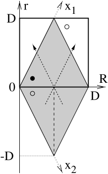
Figure 17: Re-definition of the domain of variation for $\bf R$ and $\bf r$ in one dimension. The gray area is the original domain $0<{\bf x}_{1},{\bf x}_{2}<D$ with periodic BCs. Moving the part where $R<0$ to the upper triangles, the new domain becomes $0<\vec{R,r}<D$ with periodic BCs. The bottom left empty circle, which is the $x_{1}\leftrightarrow x_{2}$ exchange counterpart of the solid circle, goes to the empty circle in the upper right triangle.

It is convenient to redefine the domain where $\bf R$ and $\bf r$ vary such that it becomes again a $2d$ torus. Fig. 17 shows how it can be done in one dimension. This change of domain modifies the usual symmetry requirement

$$\Psi(R,r)=\Psi(x_{1},x_{2})=-\Psi(x_{2},x_{1})=-\Psi(R,-r),$$ (54)

for spinless fermions, since $\psi(R,-r)\rightarrow\Psi(R+D/2,-r+D)$. In two dimensions, the symmetry requirement for spinless fermions after this change of domain becomes:

$$\Psi({\bf R},{\bf r})=-\Psi\left({\bf R}+\left({D\over 2},{D\over 2}\right),-{\bf r}+(D,D)\right).$$ (55)

The eigenstates of $H_{c}=H_{c}({\bf R})+H_{c}({\bf r})$ take the form:

$$\Psi({\bf R},{\bf r})={1\over D}e^{i{\bf KR}}\psi({\bf r}),$$ (56)

the symmetry requirement for $\psi({\bf r})$ being:

$$\psi({\bf r})=\cases{-\psi\Bigl{(}(D,D)-{\bf r}\Bigr{)},&for $\frac{D}{2\pi}(K_{x}+K_{y})$ even;\cr\psi\Bigl{(}(D,D)-{\bf r}\Bigr{)},&for $\frac{D}{2\pi}(K_{x}+K_{y})$ odd.}$$ (57)

When a sufficient Coulomb repulsion yields small oscillation of the inter-particle spacing around its largest possible value, the Coulomb repulsion can be expanded and one gets for the relative motion of the two particles a $2d$ harmonic oscillator Hamiltonian:

$$H_{c}({\bf r})=-{\hbar^{2}\over m}\nabla_{\bf r}^{2}+{e^{2}\pi\over D\sqrt{2}}+{e^{2}\pi^{3}\over D^{3}\sqrt{32}}\left|{\bf r}-\left({D\over 2},{D\over 2}\right)\right|^{2}.$$ (58)

For a $2d$ harmonic oscillator

$$H_{osc}=-{\hbar^{2}\over 2m}\nabla_{\bf r}^{2}+{m\omega^{2}\over 2}|\vec{r}|^{2},$$ (59)

the symmetric and antisymmetric GSs of energies $E_{0S}=\hbar\omega$ and $E_{0A}=2\hbar\omega$ are given by:

$$\Psi_{0S}({\bf r})=\frac{1}{l_{0}\sqrt{\pi}}\exp\left(-\frac{|{\bf r}|^{2}}{2l_{0}^{2}}\right)$$ (60)

and

$$\Psi_{0A}(\vec{r})=\frac{r_{x}\sqrt{2}}{l_{0}^{3/2}\sqrt{\pi}}\exp\left(-\frac{|\vec{r}|^{2}}{2l_{0}^{2}}\right)$$ (61)

respectively. The length $l_{0}=\sqrt{{\hbar}/({m\omega})}$ becomes in our case

$$l_{0}=\left({\hbar^{2}\over m}{\sqrt{32}D^{3}\over e^{2}\pi^{3}}\right)^{-1/4}.$$ (62)

Discretizing the continuous Hamiltonian on $L\times L$ lattice, one gets

$$H_{l} = -t\sum_{\left<{\bf j},{\bf j^{\prime}}\right>}c_{\bf j}^{\dagger}c_{\bf j^{\prime}}+4Nt$$ (63)

$$+{U\pi\over L\sqrt{\sin^{2}{(j_{x1}-j_{x2})\pi\over L}+\sin^{2}{(j_{y1}-j_{y2})\pi\over D}}},$$

where $L=D/a$, $U=e^{2}/a$ and $t=\hbar^{2}/2ma^{2}$. The constant term $4Nt$ comes from the discretization of the Laplacians. For $H_{l}$, the characteristic length $l_{0}$ becomes

$$l_{0}=\left(\frac{8\sqrt{2}t}{UL\pi^{3}}\right)^{-1/4}D.$$ (64)

Figure 18: GS energy $E_{0}$ for two particles in a $12\times 12$ lattice as a function of $U$. We have plotted for convenience $E=E_{0}-0.185U-0.137$ (taking $t=1$) for checking the contribution $\sim U^{1/2}$ at intermediate $U$ of Eq. 67. The analytical estimate ($0.159\sqrt{U}$, dotted line) is valid for $1<U<1000$, defining the continuous Wigner regime where the relative fluctuation $u_{r}\propto r_{s}^{-1/4}$ (Fig 1).

Since $l_{0}\propto r_{s}^{-1/4}D$ in our model, one gets $\left<r\right>={\sqrt{2}}D$ for the average inter-particle spacing and $\Delta r\propto r_{s}^{-1/4}D$ for the width of its distribution. Therefore, the ratio $u_{r}$ of these two quantities decays as $r_{s}^{-1/4}$. This corresponds to the behaviors shown in Fig. 1 when $r_{s}^{F}<r_{s}<r_{s}^{*}$.

For a GS of total momentum ${\bf K}=2\pi/D(1,0)$, the condition (57) yields the symmetric GS for $H_{c}({\bf r})$. For the two particle GS of $H_{c}({\bf R})+H_{c}({\bf r})$, one gets an energy

$$E_{0}={\hbar^{2}\over 4m}{\bf K}^{2}+{e^{2}\pi\over D\sqrt{2}}+\hbar\omega,$$ (65)

where

$$\hbar\omega=\sqrt{{4\hbar^{2}\over m}{1\over 2}{e^{2}\pi^{3}\over D^{3}\sqrt{8}}}.$$ (66)

This energy becomes for the corresponding lattice Hamiltonian $H_{l}$:

$$E_{0}={2\pi^{2}\over L^{2}}t+{U\pi\over L\sqrt{2}}+\sqrt{{Ut\over L^{3}}{4\pi^{3}\over\sqrt{8}}}.$$ (67)

A numerical check of this expression using a $12\times 12$ lattice model is shown in Fig. 18. Dividing $E_{0}$ by $U^{2}/t$, one gets

$$\frac{E_{0}t}{U^{2}}=\frac{\pi}{4r_{s}^{2}}+\frac{\sqrt{\pi}}{4r_{s}}+\frac{\pi^{3/4}}{4r_{s}^{3/2}}.$$ (68)

This expansion is similar to the original expression given by Wigner wigner for the strong coupling limit, the energy being measured in Rydberg units. The first term gives the kinetic energy of the center of mass ($\sim r_{s}^{-2}$), the second is the electrostatic energy at equilibrium ($\sim r_{s}^{-1}$) and the third term comes from the oscillations of the inter-particle spacing around equilibrium ($\sim r_{s}^{-3/2}$).

Appendix B Correlated lattice limit when $L\rightarrow\infty$

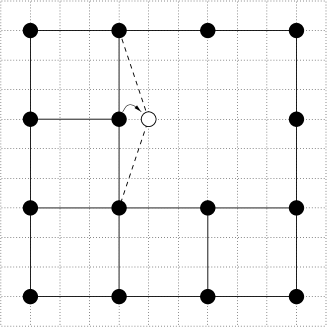
Figure 19: $N=n^{2}-1$ spinless fermions on a square lattice of size $L=3n$ for $n=4$. One of the $L^{2}$ square Wigner lattices with a vacancy of energy $E_{0}^{(0)}$ (solid circles) and one virtual state of energy $E_{1}^{(0)}$ (empty circle) contributing to the vacancy dynamics are indicated.

We study two limits which can be easily described by the $t/U$ lattice perturbation theory when $t\rightarrow 0$ and $L\rightarrow\infty$.

We keep $N=3$ spinless fermions in the first limit. In this case, the hopping term $\sim h$ characterizing the rigid translation of the molecule remains of order $t^{3}/U^{2}$, while the hopping term $\sim r$ characterizing a single particle hop over $L/2$ sites and coupling triangles of different orientations becomes of order $t(t/U)^{L/2-1}$. When $L\rightarrow\infty$, only the rigid translation of the triangle matters, and the effective Hamiltonian (Eq. 16) reads:

$$H_{eff}^{(III)}=\sum_{\bf j}E_{0}^{(II)}D_{\bf j}^{\dagger}D_{\bf j}+h\sum_{\left<{\bf j},{\bf j^{\prime}}\right>}D_{\bf j}^{\dagger}D_{\bf j^{\prime}},$$ (69)

where $D^{\dagger}_{\bf j}$ ($D_{\bf j}$) creates (annihilates) a triangle defined by Eq. 15, replacing $3$ by $L/2$. The resulting energies are:

$$E^{(III)}_{\bf K}={E}_{0}^{(II)}+2h\left(\cos K_{x}+\cos K_{y}\right),$$ (70)

yielding a GS total momentum ${\bf K}=(0,0)$.

Figure 20: The number of negative components $N_{n}(0)$ as a function of $r_{s}$. The solid line is obtained with a threshold $\zeta=10^{-12}$. The dotted line is a guide to the eyes.

We take $N=n^{2}-1$ spinless fermions and a size $L=3n$ in the second limit. $N=n^{2}$ gives a uniform filling factor $\nu=1/9$ and a square Wigner lattice which is commensurate with the assumed lattice. Taking a single particle out $n^{2}$ will create a single vacancy in the square Wigner lattice, as shown in Fig. 19. In this second limit, this is now the rigid translation of the Wigner lattice which becomes negligible in the thermodynamic limit, while the hopping term $r$ characterizing the propagation of the vacancy remains $\propto t^{3}/U^{2}$. The effective Hamiltonian (Eq. 16) takes the form:

$$H_{eff}^{(III)}=\sum_{\bf j}E_{0}^{(II)}D_{\bf j}^{\dagger}D_{\bf j}+r\sum_{\left<{\bf j},{\bf j^{\prime}}\right>_{3}}D_{\bf j}^{\dagger}D_{\bf j^{\prime}}.$$ (71)

There is only a set of virtual states of energy $E_{1}^{(0)}$ which contribute at the lowest order to the propagation of the vacancy (see Fig. 19), making simple to calculate $r$. After Fourier transformation, the eigenenergies of the effective Hamiltonian are given by:

$$E^{(III)}_{\bf K}=E_{0}^{(II)}+{2t^{3}\left(\cos 3K_{x}+\cos 3K_{y}\right)\over\left(E_{1}^{(0)}-E_{0}^{(0)}\right)^{2}},$$ (72)

and corresponds to the spectrum of a single particle on the assumed square lattice with third nearest neighbor hopping. Of course, this one vacancy dynamics does not totally remove the $L^{2}$ GS degeneracy of the limit $t\rightarrow 0$, but makes very simple the study of charge propagation in this highly correlated many particle system.

Appendix C Nodal structure of the three particle system

Figure 21: The number of negative components $N_{n}(\infty)$ as a function of $r_{s}$. The solid line is obtained with a threshold $\zeta=10^{-15}$. The dotted line is a guide to the eyes.

Figure 22: Occupation numbers $P_{\bf k}$ on the reciprocal lattice ($2\pi k_{x}/L,2\pi k_{y}/L$) for $r_{s}=0.1$ (upper figure), $r_{s}=10$ (middle figure) and $r_{s}=40$ (lower figure).

The quantum Monte-Carlo (QMC) methods are the most powerful tools for studying large many-body systems ceperley . However, the study of the ground state of fermionic systems suffers from the well known “sign problem”. One way to avoid the negative weights that would be otherwise generated by antisymmetric states is the fixed node approximation ceperley . The fixed node GS energy is then an upper bound to the exact GS energy. The nodal structure of the liquid limit is given by a simple Slater determinant of plane waves, and of localized orbitals for the solid limit. To know the exact nodal structure for intermediate couplings is not an easy problem ceperley-node . In this appendix, we study the nodal structure of three spinless fermions on a $6\times 6$ lattice.

Previously, we have considered ${\bf K}$-eigenstates, for an interacting system which is invariant under lattice translations. The Hamiltonian being invariant under time-reversal symmetry, one first define eigenvectors with real components in the site basis. For this purpose, we combine the $\bf K$-eigenvector

$$\left|\Psi_{\bf K}(r_{s})\right>=\sum_{{\bf k}_{1},{\bf k}_{2},{\bf k}_{3}\atop{\bf k}_{1}+{\bf k}_{2}+{\bf k}_{3}={\bf K}}\Psi_{{\bf k}_{1},{\bf k}_{2},{\bf k}_{3}}(r_{s})c^{\dagger}_{{\bf k}_{1}}c^{\dagger}_{{\bf k}_{2}}c^{\dagger}_{{\bf k}_{3}}\left|0\right>,$$ (73)

with its time reversed conjugate $-\bf K$-eigenvector:

$$\left|\Psi_{-{\bf K}}(r_{s})\right>=\sum_{{\bf k}_{1},{\bf k}_{2},{\bf k}_{3}\atop{\bf k}_{1}+{\bf k}_{2}+{\bf k}_{3}={\bf K}}\Psi_{{\bf k}_{1},{\bf k}_{2},{\bf k}_{3}}(r_{s})c^{\dagger}_{-{\bf k}_{1}}c^{\dagger}_{-{\bf k}_{2}}c^{\dagger}_{-{\bf k}_{3}}\left|0\right>.$$ (74)

Since the $\Psi_{{\bf k}_{1},{\bf k}_{2},{\bf k}_{3}}(r_{s})$ are real, the combination

$$\Psi_{{\bf j}_{1},{\bf j}_{2},{\bf j}_{3}}(r_{s})={1\over\sqrt{2}}\left<0\right|c_{{\bf j}_{3}}c_{{\bf j}_{2}}c_{{\bf j}_{1}}\Bigl{(}\left|\Psi_{\bf K}(r_{s})\right>+\left|\Psi_{-{\bf K}}(r_{s})\right>\Bigr{)}$$ (75)

is indeed real in the site basis.

We want to compare the nodal structure of this real GS at intermediate values of $r_{s}$ to the two limiting nodal structures, characterizing the GS either in the limit $r_{s}\rightarrow 0$ or $r_{s}\rightarrow\infty$. We define the components of a vector $\chi(r_{s},lim)$ by

$$\chi_{{\bf j}_{1},{\bf j}_{2},{\bf j}_{3}}(r_{s},lim)=\Psi_{{\bf j}_{1},{\bf j}_{2},{\bf j}_{3}}(r_{s})\cdot\Psi_{{\bf j}_{1},{\bf j}_{2},{\bf j}_{3}}(lim);$$ (76)

where $\Psi(lim)$ is the corresponding limiting GS, and we count the number $N_{n}(lim)$ of negative components of $\chi$. If the nodal structures of the limit and at $r_{s}$ are identical, $N_{n}(lim)=0$. However, when $\chi_{{\bf j}_{1},{\bf j}_{2},{\bf j}_{3}}(r_{s},lim)$ is almost zero, its sign becomes undefined due to numerical precision. This is why we ignore all the components of $\chi$ below a given threshold $\zeta$. The behavior of $N_{n}(0)$ ($N_{n}(\infty)$) where $\Psi(lim)$ is a liquid GS $\Psi(r_{s}=0.1)$ (solid GS $\Psi(r_{s}=10^{3})$) is shown in Fig. 20 (Fig. 21).

As one can see, the nodal structure does not exhibit a sharp transition between the two limits, but a crossover with complex intermediate behaviors. Notably, there are some plateau values suggesting some constant nodal structure around the intermediate values of $r_{s}$ where we observe the PMWM states. This illustrates the difficulty to use a fixed node Monte-Carlo method for describing the intermediate GS on a lattice.

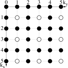
Figure 23: Above: Occupation numbers $P_{\bf k}$ for $r_{s}=500$. Below: Occupation numbers $P_{\bf k}$ at $r_{s}=\infty$, showing the two possible values $1/9$ (filled circles) and $0$ (empty circles).

Appendix D Occupation numbers in ${\bf k}$-space

It is not only interesting to know how the system occupies the real lattice, but also the reciprocal lattice. From the GS wave function $\Psi_{0}(r_{s})$ of total momentum ${\bf K}=2\pi/6(1,1)$, we have calculated the occupation numbers

$$P_{\bf k}(r_{s})=\left<\Psi_{0}(r_{s})\right|d^{\dagger}_{\bf k}d_{\bf k}\left|\Psi_{0}(r_{s})\right>,$$ (77)

in ${\bf k}$-space. Fig. 22 and Fig. 23 give plots of those number in the reciprocal lattice for increasing values of $r_{s}$. When $r_{s}\rightarrow 0$, only three ${\bf k}$-states are occupied (Fig. 22). When $r_{s}\rightarrow\infty$, one gets a simple pattern (Fig. 23) for ${\bf K}=2\pi/6(1,1)$, which can be analytically obtained:

$$P_{\bf k}(r_{s}=\infty)=\cases{0&if ${\bf k}=2\pi/6\times$(odd,odd)\cr 1/9&else}.$$ (78)

Between the two limits, the occupation numbers $P_{\bf k}$ of the two identified PMWMs ($r_{s}=10$ and $r_{s}=40$) have a mixed character, where both the “solid” and the “liquid” patterns are visible when one uses a logarithmic scale. This is what one should expect when a “supersolid” is forming: the usual spreading of the “Fermi sea” being accompanied by the gradual emergence of the Fourier spectrum of the “Wigner solid”.

References

- (1) A. F. Andreev and I. M. Lifshitz, Sov. Phys. JETP 29, 1107 (1969).
- (2) E. Abrahams, S. V. Kravchenko and M. P. Sarachik, Rev. Mod. Phys. 73, 251 (2001) and refs therein.
- (3) D. H. Dubin and T. M. O’Neil, Rev. Mod. Phys. 71, 87 (1999).
- (4) G. Katomeris, F. Selva and J.-L. Pichard, Eur. Phys. J. B. 31, 401 (2002).
- (5) J. P. Bouchaud and C. Lhuillier, Europhys. Lett. 3, 481 (1987) and Europhys. Lett. 3, 1273 (1987); J. P. Bouchaud, A. Georges and C. Lhuillier, J. Phys. France 49, 553 (1988).
- (6) F. Selva and J.-L. Pichard, Europhys. Lett. 55, 518 (2001).
- (7) Z. Á. Németh and J.-L. Pichard, Europhys. Lett. 58, 744 (2002).
- (8) M. Martínez and J.-L. Pichard, Eur. Phys. J. B. 30, 93 (2002).
- (9) E. Wigner, Trans. Faraday Soc. 34, 678 (1938).
- (10) W. J. Carr, Phys. Rev. 122, 1437 (1961).
- (11) D. Weinmann and J.-L. Pichard, Phys. Rev. Lett. 77, 1556 (1996).
- (12) D. L. Shepelyansky and O. P. Sushkov, Europhys. Lett. 37, 121 (1997)
- (13) D. Weinmann, J.-L. Pichard and Y. Imry, J. Phys. I France 7, 1559 (1997).
- (14) B. L. Altshuler, Y. Gefen, A. Kamenev and L. Levitov, Phys. Rev. Lett. 78, 2803 (1997).
- (15) P. Jacquod and D. L. Shepelyansky, Phys. Rev. Lett. 79, 1837 (1997).
- (16) V. V. Flambaum, F. M. Izrailev, and G. Casati, Phys. Rev. E 54, 2136 (1996).
- (17) B. Tanatar and D.M. Ceperley, Phys. Rev. B 39, 5005 (1989); Ladir Cândido, Philip Philipps and D. M. Ceperley, Phys. Rev. Lett. 86, 492 (2001); C. Attaccalite, S. Moroni, P. Gori-Giorgi and G. B. Bachelet, Phys. Rev. Lett. 88, 256601 (2002).
- (18) D.M. Ceperley, J. Stat. Phys 63, 1237 (1991.)