Renormalization group method for weakly-coupled quantum chains: application to the spin one-half Heisenberg model

Abstract

The Kato-Bloch perturbation formalism is used to present a density-matrix renormalization-group (DMRG) method for strongly anisotropic two-dimensional systems. This method is used to study Heisenberg chains weakly coupled by the transverse couplings $J_{\perp}$ and $J_{d}$ ( along the diagonals). An extensive comparison of the renormalization group and quantum Monte Carlo results for parameters where the simulations by the latter method are possible shows a very good agreement between the two methods. It is found, by analyzing ground state energies and spin-spin correlation functions, that there is a transition between two ordered magnetic states. When $J_{d}/J_{\perp}\lesssim 0.5$, the ground state displays a Néel order. When $J_{d}/J_{\perp}\gtrsim 0.5$, a collinear magnetic ground state in which interchain spin correlations are ferromagnetic becomes stable. In the vicinity of the transition point, $J_{d}/J_{\perp}\approx 0.5$, the ground state is disordered. But, the nature of this disordered ground state is unclear. While the numerical data seem to show that the chains are disconnected, the possibility of a genuine disordered two-dimensional state, hidden by finite size effects, cannot be excluded.

I Introduction

In a recent publication TS1-moukouri , it was shown that the density-matrix renormalization group method (DMRG) white ; DMRG-book can be applied to an array of weakly coupled quantum chains. As an illustration of the method, weakly coupled Heisenberg spin chains were studied and some partial results on the ground state energies were shown to be in good agreement with previous quantum Monte Carlo (QMC) studies. But the essential question concerning the stability of the disordered one-dimensional (1D) ground state against small transverse perturbations was not addressed.

The motivation behind such a study is in the search of a disordered ground state for a spin one-half Heisenberg model in dimension higher than one. A spin liquid state without spin rotational or translational symmetry breaking has been conjectured to be relevant for the physics of high-Tc cuprate superconductors anderson1 . A possible candidate is the resonance valence bond (RVB) state anderson . Earlier attempts chandra1 ; dagotto ; chandra2 ; sorella to find the RVB ground state by various techniques ($1/S$ expansions, exact diagonalization, quantum Monte Carlo) have given some indication about its possible realization. But their conclusions are still disputed. It has even been argued read that the spin-Peierls mechanism, not RVB, may be the most natural way to lead to a disordered state.

More recently, the interest has shifted to search for a RVB state on quasi 1D systems. A pure spin one-half Heisenberg chain has a disordered ground state with neutral spin one-half excitations (spinons) and does not break spin rotational or translational symmetry. It is thus tempting to try to find a higher dimensional generalization of this state by the application of small perturbations. Contrary to an earlier claim of the realization of a spin liquid parola , subsequent studies affleck ; rosner ; sandvik2 indicate that the introduction of the rung transverse coupling $J_{\perp}$ between the chains (see Fig. 1) seems to lead to a Néel state for any non-zero $J_{\perp}$. A possible way to avoid the Néel order is to introduce, in addition to $J_{\perp}$, a small frustration $J_{d}$ along the diagonals. In a recent work tsvelik it was claimed that a spin liquid state is realized when $J_{\perp}=2J_{d}$.

A more direct motivation in studying a model of weakly coupled Heisenberg chains stems to its relevance to the understanding of interchain effects in quasi-one-dimensional materials sajita ; keren ; tennant . A recent neutron scattering experiment coldea on the frustrated antiferromagnet (AFM) $Cs_{2}CuCl_{4}$ found that the dynamical correlation show a highly dispersive continuum of a excitations with fractional quantum numbers, a signature of a spin liquid state.

Figure 1: Sketch of the ground state of weakly coupled Heisenberg chains as function of $J_{\perp}$ (dashed lines along the rungs) and $J_{d}$ (dotted lines along the diagonals): Néel state when $J_{d}/J_{\perp}\lesssim 0.5$ (left), collinear state when $J_{d}/J_{\perp}\gtrsim 0.5$ (right)

In this paper, a general formalism of the DMRG algorithm for weakly coupled chains of Ref.TS1-moukouri is presented. This method is a particular case of a recent matrix version MAT-moukouri of the general perturbation expansion which was proposed decades ago by Kato and Bloch kato ; bloch ; messiah . The Kato-Bloch expansion was initially introduced to find the correction on a single state. This expansion is straightforwardly generalized to account for many low lying states. The method is in spirit close to an earlier perturbative renormalization group by Hirsch and Mazenko hirsch . A more detailed study of weakly coupled Heisenberg chains is presented. An extensive comparison with quantum Monte Carlo results for unfrustrated transverse couplings is made. It shows a good agreement between the two methods when the perturbation is small and the lattice not too large. Then the question of the stability of the non-magnetic state in the presence of frustration is addressed. It is shown that the 2D DMRG algorithm can provide a convincing answer to this question, at least for the parameters that were investigated. It is found, by analyzing ground state energies and spin-spin correlation functions, that the perturbation is relevant, leading to magnetic ground states (see Fig. 1). When $J_{d}/J_{\perp}\lesssim 0.5$, the ground state displays a Néel order. When $J_{d}/J_{\perp}\gtrsim 0.5$ a collinear magnetic ground state in which interchain spin correlations are ferromagnetic becomes stable. In the vicinity of the transition point, $J_{d}/J_{\perp}\approx 0.5$, the system seems to behave as an assembly of independent chains. This is reminescent of the so-called sliding Luttinger liquid lubensky recently found in a model of crossed spin one-half Heisenberg chains singh . But it is impossible to exclude a genuine 2D spin liquid state (i.e., with a spin gap) masked by finite size effects.

II Formal development

The DMRG method described below can work for spin, fermionic as well as bosonic systems, and so it is convenient to use a general formulation of the algorithm that can then be adapted to each of these cases. The model Hamiltonians under consideration can be written as follows:

$$H=H_{\parallel}+gH_{\perp},$$ (1)

where $H_{\parallel}$ is a the sum over one-dimensional (1D) Hamiltonians (longitudinal direction),

$$H_{\parallel}=\sum_{l=1}^{L}H_{l},$$ (2)

and $H_{\perp}$ is the interaction between these 1D systems (transverse direction). The coupling constant $g$ is such that $g\ll 1$.

Since $g\ll 1$, it is natural to study the problem using perturbation theory. The Kato-Bloch formalism is convenient to set up a perturbation expansion around a numerical solution of $H_{\parallel}$ provided by the DMRG. For a single chain $l$ whose Hamiltonian is $H_{l}$, a set of eigenstates $|\phi_{n_{l}}\rangle$ and eigenvalues $\epsilon_{n_{l}}$ can be obtained by the usual 1D DMRG. The zeroth order set of eigenstates $|\Phi_{\parallel[n]}\rangle$ of the full longitudinal Hamiltonian is simply given by the tensor product of the $|\phi_{n_{l}}\rangle$,

$$|\Phi_{\parallel[n]}\rangle=|\phi_{n_{1}}\rangle|\phi_{n_{2}}\rangle...|\phi_{n_{L}}\rangle,$$ (3)

and the set of approximate eigenvalues of $H_{\parallel}$ is given by the sum

$$E_{\parallel[n]}=\epsilon_{n_{1}}+\epsilon_{n_{2}}+...+\epsilon_{n_{L}},$$ (4)

where $[n]=(n_{1},n_{2},...,n_{L})$ and $n_{l}$ labels to an eigenset on the chain $l$.

Let $P_{\parallel}$ be the projector on the states $|\Phi_{\parallel[n]}\rangle$,

$$P_{\parallel}=\sum_{[n]}|\Phi_{\parallel[n]}\rangle\langle\Phi_{\parallel[n]}|$$ (5)

and $Q_{\parallel}=1-P_{\parallel}$.

Let ($E_{[n]}$, $|\Phi_{[n]}\rangle$) be the exact eigenset of $H$. This eigenset will tend to ($E_{\parallel[n]}$, $|\Phi_{\parallel[n]}\rangle$) in the limit $g\rightarrow 0$. Let $P$ be the projector onto the spaces $|\Phi_{[n]}\rangle$. $P$ may be written as follows

$$P=\sum_{[n]}|\Phi_{[n]}\rangle\langle\Phi_{[n]}|.$$ (6)

Since the perturbation $g$ is small, it is assumed that the subspaces generated by the $|\Phi_{\parallel[n]}\rangle$’s and by the $|\Phi_{[n]}\rangle$’s are not orthogonal. An approximate expression of $HP$ in the basis spanned by the eigenstates of $H_{\parallel}$ will now be derived by using a generalization of a method first introduced by Kato kato and later modified by Bloch bloch . The advantage of the Bloch’s version is that it leads to a simpler expansion.

Following Bloch, let ${\cal U}$ be the operator

$${\cal U}=\sum_{[n]}|\Phi_{[n]}\rangle\langle\Phi_{\parallel[n]}|$$ (7)

which projects the $|\Phi_{\parallel[n]}\rangle$ onto $|\Phi_{[n]}\rangle$, and ${\cal U}$ satifies, ${\cal U}P_{\parallel}={\cal U}$. The problem of finding an expansion of $HP$ projected onto $P_{\parallel}$ is equivalent to finding an expansion for $P_{\parallel}H{\cal U}$.

One starts by deriving an equation satisfied by ${\cal U}$. The Schrödinger equation

$$H|\Phi_{[n]}\rangle=E_{[n]}|\Phi_{[n]}\rangle$$ (8)

is transformed as follows,

$$(H-{\tilde{H}}_{\parallel})|\Phi_{[n]}\rangle={\cal E}_{[n]}|\Phi_{[n]}\rangle$$ (9)

where ${\tilde{H}}_{\parallel}$ is identical to $H_{\parallel}$ in the subspace spanned by the $|\Phi_{\parallel[n]}\rangle$’s, and,

$${\cal E}_{[n]}=E_{[n]}-\langle\Phi_{[n]}|{\tilde{H}}_{\parallel}|\Phi_{[n]}\rangle.$$ (10)

When a single state $|\Phi_{\parallel[0]}\rangle$ is kept, ${\tilde{H}}_{\parallel}$ is given by

$${\tilde{H}}_{\parallel}=\left(\begin{array}[]{ccccccc}E_{\parallel[0]}&0&0&0&0&\ldots&0\\ 0&E_{\parallel[0]}&0&0&0&\ldots&0\\ 0&0&E_{\parallel[0]}&0&0&\ldots&0\\ &&\ldots&&&\ldots&\\ 0&0&\ldots&E_{\parallel[0]}&&\ldots&\\ 0&0&0&\ldots&E_{\parallel[0]}&\ldots&0\\ &&\ldots&&&\ldots&\\ 0&0&0&0&0&\ldots&E_{\parallel[0]}\\ \end{array}\right).$$ (19)

The method reduces to the usual stationary perturbation expansion. It is known that such an expansion does not often converge. The main source of divergence is the near degeneracy of the eigenvalues. Now if many states up to a cut-off $n_{c}$ are kept, a possible generalization of ${\tilde{H}}_{\parallel}$ to many states $|\Phi_{\parallel[0]}>\ldots|\Phi_{\parallel[n_{c}]>}$, is

$${\bar{H}}_{\parallel}=\left(\begin{array}[]{ccccccc}E_{\parallel[0]}&0&0&0&0&\ldots&0\\ 0&E_{\parallel[1]}&0&0&0&\ldots&0\\ 0&0&E_{\parallel[2]}&0&0&\ldots&0\\ &&\ldots&&&\ldots&\\ 0&0&\ldots&E_{\parallel[n_{c}]}&&\ldots&\\ 0&0&0&\ldots&E_{\parallel[0]}&\ldots&0\\ &&\ldots&&&\ldots&\\ 0&0&0&0&0&\ldots&E_{\parallel[0]}\\ \end{array}\right).$$ (28)

Thus if $n_{c}$ is suitably chosen, the series will converge MAT-moukouri . The purpose of this choice is to shield the eigenvalue $E_{\parallel[0]}$ from the rest of the spectrum by treating the $n_{c}-1$ states just above the ground state exactly and the remaining spectrum perturbatively.

By applying $P_{\parallel}$ and then ${\cal U}$ to the Equation( 9) above, one finds,

$$g{\cal U}H_{\perp}|\Phi_{[n]}\rangle={\cal E}_{[n]}|\Phi_{[n]}\rangle$$ (29)

The subtraction of Equation( 29) from Equation( 9) leads to

$$(H-{\tilde{H}}_{\parallel}-g{\cal U}H_{\perp})|\Phi_{[n]}\rangle=0.$$ (30)

By applying $\langle\Phi_{\parallel[n]}|$ on the right of equation( 30) and performing the summation over $[n]$ , one finally obtains the equation satisfied by ${\cal U}$,

$$(H-{\tilde{H}}_{\parallel}-g{\cal U}H_{\perp}){\cal U}=0.$$ (31)

Equation( 31) is further transformed by using the fact that $P_{\parallel}{\cal U}=P_{\parallel}$ and ${\cal U}=P_{\parallel}{\cal U}+Q_{\parallel}{\cal U}$. One obtains:

$${\cal U}=P_{\parallel}+g{\tilde{Q}}_{\parallel}(H_{\perp}{\cal U}-{\cal U}H_{\perp}{\cal U})$$ (32)

where $\tilde{Q_{\parallel}}$ is given by

$$\tilde{Q_{\parallel}}=Q_{\parallel}({\tilde{H}}_{\parallel}-H_{\parallel})^{-1}.$$ (33)

This leads to the expansion for ${\cal U}$

$${\cal U}^{(0)}=P_{\parallel}$$ (34)

$${\cal U}^{(n)}=g{\tilde{Q}}_{\parallel}[H_{\perp}{\cal U}^{(n-1)}-\sum_{p=1}^{n-1}{\cal U}^{(p)}H_{\perp}{\cal U}^{(n-p-1)}]$$ (35)

From this expansion, one finds the approximate Hamiltonian ${\tilde{H}}=P_{\parallel}H{\cal U}$ is

$$\tilde{H}=\sum_{[n]}E_{\parallel[n]}|\Phi_{\parallel[n]}\rangle\langle\Phi_{\parallel[n]}|+gP_{\parallel}H_{\perp}P_{\parallel}+$$

$$g^{2}P_{\parallel}H_{\perp}\tilde{Q_{\parallel}}H_{\perp}P_{\parallel}+...$$ (36)

This perturbation expansion is a matrix generalization to many states of Bloch’s expansion bloch ; messiah which was established for a single state. Even though the ground state and a few low lying states will ultimately be computed, it is important to keep many low lying states in the perturbation expansion. This is because the convergence will mainly depend on two quantities. The first one is obviously $g$. The second one is the projector $\tilde{Q_{\parallel}}$. If ${\tilde{H}}_{\parallel}={H}_{\parallel}$, then $Q_{\parallel}=0$. In that case only the first order term in equation ( 36) is not equal to zero. The rewriting of the original problem to equation ( 36) is a simple change of basis. So in the limit where $n_{c}=dimA$, where $A$ is the Hilbert space in which all the operators are defined, the method is exact. But since only a small number of eigenstates of $H_{\parallel}$ can be used even if the full spectrum is known, $Q_{\parallel}\neq 0$. The magnitude of $\tilde{Q_{\parallel}}$ in the expansion decreases by increasing the cut-off $n_{c}$. It is to be noted this matrix expansion is close to the method of Hirsch and Mazenko hirsch , who also used a block expansion near the solution of an unperturbed Hamiltonian. The problem with their study was, however, that their technique was applied to a model with no small parameter.

When the DMRG is used as a method of solution for $H_{\parallel}$, we can not know $Q_{\parallel}$ exactly. This is because the DMRG does not keep any information about the truncated states. But it is possible to define a perturbative expansion in a reduced space spanned by the states kept. The above perturbative expansion will thus be adapted in this study as follows. During the 1D DMRG part of the method, $N_{s}=ms_{1}\times ms_{1}$ states will be obtained for the reduced superblock (i.e., the superblock reduced to the two external large blocks; it is supposed that open boundary conditions (OBC) are used). Typically $ms_{1}=16-192$ during this investigation. The complete spectrum of this reduced superblock can be obtained as in the thermodynamic algorithm moukouri-THERMO . This spectrum will serve as $H_{\parallel}$. Only a small fraction $ms_{2}=16-96$ of these states can be kept for the generation of the 2D lattice. The $ms_{2}$ states will define $P_{\parallel}$, and $Q_{\parallel}$ is constructed using the remaining $Ns-ms_{2}$ states. Hence the perturbation expansion in Eq.( 36) will be made by assuming that $H_{\parallel}$ is the low energy Hamiltonian of size $ms_{1}\times ms_{1}$ obtained from the DMRG rather than the exact 1D solution of $H_{\parallel}$.

The Hamiltonian $\tilde{H}$ is one-dimensional and it will be studied by the DMRG method. The only difference with a normal 1D situation is that the local operators are now $ms_{2}\times ms_{2}$ matrices which makes computations heavier. It should be noted that the accuracy of the method is related to the diagonalized unperturbed Hamiltonian obtained from the DMRG. This Hamiltonian, although it leads to a very accurate ground state energy, is less accurate for high lying states and correlation functions. So the potential errors of the method will come from the DMRG as well as the truncated perturbative series. A better approach is to use the exact diagonalization method to diagonalize the unperturbed Hamiltonian. However, in that case one will be restricted to small chains.

III Application to the Heisenberg model

The above formalism will now be applied to the anisotropic Heisenberg model on a 2D square lattice. The Hamiltonian reads:

$$H_{spins}=\sum_{i,l}{\bf S}_{i,l}{\bf S}_{i+1,l}+J_{\perp}\sum_{i,l}{\bf S}_{i,l}{\bf S}_{i,l+1}+$$

$$J_{d}\sum_{i,l}({\bf S}_{i,l}{\bf S}_{i+1,l+1}+{\bf S}_{i+1,l}{\bf S}_{i,l+1})$$ (37)

where the ${\bf S}_{i,l}$ are the usual spin one-half operators.

The question of the condition of the onset of long-range order as a function of $J_{\perp}$ has been addressed in many studies. Spin-wave analysis sakai ; parola predicted that there is a finite critical $J_{\perp c}\approx 0.03$, above which long-range order is established. Renormalization group analysis affleck supplemented by series expansion computations found that if $J_{\perp c}$ is finite, it cannot exceeds $0.02$. A finite critical value is at variance with a random phase approximation (RPA) rosner which predits $J_{\perp c}=0$. The QMC method combined with a multichain mean-field approach sandvik2 has concluded that when $J_{\perp}=0$, the ground state is an antiferromagnet down to $J_{\perp}=0.02$. From these studies, it is likely that the AFM ground state is stable as soon as $J_{\perp}\neq 0$. This does not, however, preclude a spin liquid ground state in the case when $J_{d}$ is added between the chains. When this exchange term is added, the QMC method faces the infamous sign problem. The two-step DMRG method presented here can help to find, if it exists, the spin liquid ground state.

The adaptation of the formalism discussed in section( II) to the model of Equation( 37) is without any difficulty. The first step is the solution of the 1D Hamiltonian:

$$H_{l}=\sum_{i}{\bf S}_{i,l}{\bf S}_{i+1,l}$$ (38)

by the usual DMRG method. This yields the chain eigenvalues $\epsilon_{n_{l}}$ and eigenstates $|\phi_{n_{l}}\rangle$. From equation ( 36), the projected Hamiltonian in the first order approximation is given by

$$\tilde{H}=\sum_{[n]}E_{\parallel[n]}|\Phi_{\parallel[n]}\rangle\langle\Phi_{\parallel[n]}|+J_{\perp}P_{\parallel}\sum_{i,l}{\bf S}_{i,l}{\bf S}_{i,l+1}P_{\parallel}+$$

$$J_{d}P_{\parallel}\sum_{i,l}({\bf S}_{i,l}{\bf S}_{i+1,l+1}+{\bf S}_{i+1,l}{\bf S}_{i,l+1})P_{\parallel}.$$ (39)

which may simply be written as

$$\tilde{H}\approx\sum_{[n]}E_{\parallel[n]}|\Phi_{\parallel[n]}\rangle\langle\Phi_{\parallel[n]}|+J_{\perp}\sum_{il}{\bf\tilde{S}}_{i,l}{\bf\tilde{S}}_{i,l+1}+$$

$$J_{d}\sum_{il}({\bf\tilde{S}}_{i,l}{\bf\tilde{S}}_{i+1,l+1}+{\bf\tilde{S}}_{i+1,l}{\bf\tilde{S}}_{i,l+1}),$$ (40)

where ${\bf{\tilde{S}}}_{i,l}^{n_{l},m_{l}}=\langle\phi_{n_{l}}|{\bf S}_{i,l}|\phi_{m_{l}}\rangle$.

The matrix elements for the second terms may be written

$$\langle\Phi_{\parallel[n]}|H_{\perp}{\tilde{Q}}_{\parallel}H_{\perp}|\Phi_{\parallel[n^{\prime}]}\rangle=\sum_{il,i^{\prime}l^{\prime},[m]}\frac{\langle\Phi_{\parallel[n]}|{\bf S}_{i,l}{\bf S}_{i,l+1}|\Phi_{\parallel[m]}\rangle\langle\Phi_{\parallel[m]}|{\bf S}_{i,l}{\bf S}_{i,l+1}|\Phi_{\parallel[n^{\prime}]}\rangle}{E_{\parallel[0]}-E_{\parallel[m]}}$$ (41)

The second order term ( 41) generates a long-range coupling between the chains, which makes it difficult to treat. One can see that the condition for the matrix element to be non zero is that $\langle\phi_{n_{l1}}|\phi_{m_{l2}}\rangle=\delta_{n_{l1},m_{l2}}$ except when $l_{1,2}=l$ or $l+1$. Thus,

$$E_{[m]}-E_{[0]}=(\epsilon_{n_{1}}-\epsilon_{0_{1}})+...+(\epsilon_{m_{l}}-\epsilon_{0_{l}})+(\epsilon_{m_{l+1}}-\epsilon_{0_{l+1}})+...+(\epsilon_{n_{L}}-\epsilon_{0_{L}}).$$ (42)

In the Eq. 42 above, the dominant terms will come from the differences involving the indices $m_{l}$ and $m_{l+1}$ because the others terms come from the state used to generate $P_{\parallel}$ and are thus of lower energies. Up to the second order, the effective one-dimensional Hamiltonian, which is written here without the frustration term, is

$$\tilde{H}\approx\sum_{[n]}E_{\parallel[n]}|\Phi_{\parallel[n]}\rangle\langle\Phi_{\parallel[n]}|+J_{\perp}\sum_{l}{\bf\tilde{S}}_{l}{\bf\tilde{S}}_{l+1}-$$

$$\frac{J_{\perp}^{2}}{2}\sum_{l}{\bf S}_{l}^{(2)}{\bf S}_{l+1}^{(2)}+...$$ (43)

where the chain-spin operators on the chain $l$ are ${\bf\tilde{S}}_{l}=({\bf\tilde{S}}_{1l},{\bf\tilde{S}}_{2l},...{\bf\tilde{S}}_{Ll})$ and ${\bf S}_{il}^{(2)}=({\bf\tilde{S}}_{1l}^{(2)},{\bf\tilde{S}}_{2l}^{(2)},...{\bf\tilde{S}}_{Ll}^{(2)})$, $L$ is the chain length. The matrix elements of the second order local spin operators are

$${\bf S}_{il}^{(2)n_{l}n^{\prime}_{l}}=\sum_{m_{l}}\frac{{\tilde{S}}_{il}^{n_{l}m_{l}}{\tilde{S}}_{il}^{m_{l}n^{\prime}_{l}}}{\sqrt{\epsilon_{m_{l}}-\epsilon_{0_{l}}}}.$$ (44)

One can note that this expression of ${\bf S}_{il}^{(2)}$ is not exact, it has been simplified to avoid long-range coupling between the chains. The effective 1D Hamiltonian $\tilde{H}$ is also studied using DMRG.

IV Algorithmic details

The algorithm of the method will now be described below. It consists of two DMRG steps separated by an intermediate stage in which a simple block decimation is made.

IV.1 Step 1

Figure 2: sketch of the superblock in the step 1

The first step of the method is the usual DMRG method for a single chain. The chain is divided into four blocks, and the two internal blocks are made of a single site each. In the calculations, $ms_{1}=16-192$ states are kept in the two external blocks. In most cases, the initial iteration starts with a chain having the largest size before truncation, for instance $L=16$ when $ms_{1}=128$ states are kept. This way, a high accuracy is obtained even when the infinite system method is used. During this step, the local spin operators ${\bf S}_{i}$ on each site $i$ of the chain are stored and longitudinal spin-spin correlations $C(i,r)=\langle{\bf S}_{i}{\bf S}_{i+r}\rangle$ are also computed and stored. As discussed by Caron and Bourbonnais caron , open boundary conditions (OBC) which are used here introduce spurious behavior at the edges of the chain. It is therefore better to chose the origin $i$ in $C(i,r)$ in the middle of chain. It is crucial during this step to target more just than the $S_{z}=0$ sector in order to obtain a correct low-energy Hamiltonian. In addition to $S_{z}=0$, $S_{z}=\pm 1$, $\pm 2$ were targeted in this study.

IV.2 Block transformation

Figure 3: sketch of the transformation of the two external blocks of length $L/2$ into a single block of length $L$ which is used as the building unit in step 2

An intermediate stage of the algorithm is a decimation process as in the old block renormalization group method weinstein ; jullien . In this process, the two external blocks having $L/2$ sites each are reduced to a single block with $L$ sites. During this step, the $ms_{1}\times ms_{1}$ states describing the chain are reduced to $ms_{2}$ lowest states of the chain. As noted in Ref. TS1-moukouri , since the block transformation is used only one time, the problem of the propagation of spurious boundary effects white-noack is not present. All the local spin operators and spin-spin correlation functions are expressed in the basis of the $ms_{2}$ states.

IV.3 Step 2

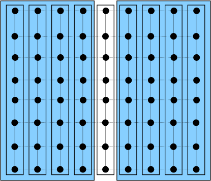
Figure 4: Sketch of the superblock in step 2

The second step consists of applying the 1D DMRG method using the chains obtained at the end of the previous step as the building blocks. This step is indeed identical to the first step, except for the dimension of the local spin operators. The central block is the chain from the previous step and thus has the dimension $ms_{2}\times ms_{2}$. Typically, $ms_{2}=16-96$ and for the two external blocks, roughly the same number of states is kept. If four blocks were taken as in the first step, the dimension of the superblock would be $ms_{2}^{4}$ which can become rapidly impratical. To ease the computations, three blocks instead of four are mostly used during this step. As will be seen below, it is important during this step to check that, for a given value of the couplings $J_{\perp}$ and $J_{d}$, enough states are kept such that a valid computation is made. i.e., that the truncated Hamiltonian generated for the single chain is accurate enough, for the ground state and for the low lying states, to be used as a building block for the 2D lattice. One can easily see that for a fixed $L$ and $J_{\perp,d}\ll\Delta_{\sigma}(L)$, $\Delta_{\sigma}(L)$ is the finite size spin gap, and the interchain matrix elements will be negligible. The system will behave as a collection of free chains even if $J_{\perp,d}$ is turned on. Now if $J_{\perp,d}\sim\delta E(L)$, where $\delta E(L)$ is the width of the retained states, the matrix elements of the states having higher energy, which have been truncated out, have a non-negligible contribution.

IV.4 Algorithm

The algorithm is summarized below.

• 1. Build the low energy Hamiltonian for a single chain $B\cdot\cdot B$ by using the 1D DMRG algorithm of Refwhite . Store the spin operator ${\bf S}_{i}$ on each site and the correlation function $C(i,r)$.

• 2. When the block $B$ size is $L/2$, apply the block method to merge the two external blocks into a single block defined by the $ms_{2}$ states kept. Express all the spin operators and correlation functions in the basis of the $ms_{2}$ states. Check if for the number of states kept, the transverse couplings satisfy $\Delta_{\sigma}(L)\lesssim J_{\perp,d}\ll\delta E(L)$. If this condition is not satisfied, increase $ms_{2}$.

• 3. Start a second 1D DMRG simulation identical to the first one except that the central block is now a single chain instead of a site, and the exchange coupling is $J_{\perp,d}$ instead of $1.0$.

V Results with four blocks in step 2

In this part, the DMRG results are compared to the stochastic series expansion (SSE) QMC results. The SSE-QMC method sandvik1 is so far the most reliable technique for the study of quantum spin systems. It has been used to study weakly coupled quantum spin chains sandvik2 . It will thus be very instructive to see how well the DMRG method compares to the SSE-QMC.

V.1 First order ground-state energies

In Table ( 1), the ground state energy per site for $12\times 12$ systems for $m=16$, $24$ and $32$ is shown. In this calculation, four blocks were used in the second DMRG step. The agreement with the SSE-QMC results is good for small $g$. The DMRG energies are higher than those of the QMC for all transverse couplings studied. As $ms_{2}$ is increased, the difference between the DMRG and QMC energies decreases. This was expected since the current method as the original DMRG procedure is variational.

$J_{\perp}$	$ms_{2}=16$	$ms_{2}=24$	$ms_{2}=32$	QMC
$0.00$	-0.42848	-0.42851	-0.42851	-0.42849(2)
$0.05$	-0.42900	-0.42907	-0.42909	-0.42926(2)
$0.10$	-0.43058	-0.43078	-0.43090	-0.43147(2)
$0.15$	-0.43312	-0.43361	-0.43387	-0.43530(2)
$0.20$	-0.43642	-0.44733	-0.43780	-0.44064(2)
$0.25$	-0.44028	-0.44174	-0.44247	-0.44727(2)

Table 1: DMRG ground state energies for $12\times 12$ lattices for $ms_{1}=ms_{2}=16$, $24$, and $32$ versus QMC.

The band-width of the states kept is $\Delta E=1.132$, $1.290$, $1.466$ when $ms_{2}=16$, $24$ and $32$ respectively. The target states during the first DMRG step were the lowest states of the spin sectors with $S_{z}=0$, $\pm 1$ $\pm 2$. The lowest states of higher spin sectors have energies which are higher than the highest state kept in lower spin sectors, therefore they were not targeted. The fact that the DMRG results compare well with the QMC ones even at intermediate couplings reveals that for the spin chain, reliable calculations can be made for values of $\delta E(L)/J_{\perp}\approx 5$. But as expected for higher values of $J_{\perp}$, the condition $\delta E(L)/J_{\perp}\gg 1$ is no longer fulfilled. This means the Hilbert space is too severely truncated.

V.2 Second order ground-state energies

Table  2 displays second order ground-state energies for a $12\times 12$ system which are compared with QMC. The agreement is systematically better than in the first order case for all values of $J_{\perp}$ studied. But the improvment is small. This is because as discussed above, the DMRG does not provide the full 1D spectrum. Only the states kept to form the reduced superblock are used in the perturbative expansion. When $ms_{2}=32$, this is merely $924$ states i.e., a tiny fraction of of the $2^{144}$ states which form the full Hilbert space of the $12\times 12$ lattice. Another reason for this modest improvment is the fact that the DMRG energies are variational. The high lying energies which are used to generate second order terms are obtained with less accuracy than the states kept in the first order. Indeed, this does not mean that the matrix expansion presented above is not efficient. It has been used in the simple case of the Mathieu equation for which the full spectrum of unperturbed Hamiltonian is available MAT-moukouri . The convergence of the matrix method is quite impressive. Thus it seems that the best way to use the matrix Kato-Block expansion when the DMRG is used to obtain the unperturbed spectrum is to restrict oneself to the first order and keep $ms_{2}$ as large as possible. However, larger values of $ms_{2}$ are unpratical when four blocks are used to form the superblock in the second step. For this reason from now, only three blocks will be used to generate the superblock in the second step.

$J_{\perp}$	$ms_{2}=16$	$ms_{2}=24$	$ms_{2}=32$	QMC
$0.00$	-0.42848	-0.42851	-0.42851	-0.42849(2)
$0.05$	-0.42901	-0.42909	-0.42910	-0.42926(2)
$0.10$	-0.43063	-0.43083	-0.43094	-0.43147(2)
$0.15$	-0.43322	-0.43369	-0.43396	-0.43530(2)
$0.20$	-0.43661	-0.43746	-0.43797	-0.44064(2)
$0.25$	-0.44055	-0.44192	-0.44271	-0.44727(2)

Table 2: DMRG ground state energies for $12\times 12$ lattices for second order DMRG compared with QMC for $ms_{1}=ms_{2}=16$, $24$ and $32$.

VI First order results with three blocks in step 2

When three blocks are used, the superblock size in the second step is divided by $ms_{2}$ relative to the case of four blocks. This significantly reduces the amount of required CPU for a given value of $ms_{2}$. But this is not without problems. It was noted that white , when three blocks are used, the coupling between blocks may incorrectly sets in leading to a poor performance of the method even if the truncation errors are small. The remedy against this problem is to target more than one state so that the interblock mixture is performed correctly. However, targeting many superblock states lower the accuracy on the ground state. For this reason, only the ground state was targeted. The truncation errors were in general smaller than $10^{-8}$ for $ms_{2}$ varying from $16$ to $96$ for different lattice size. But as said above, this does not give any indication about the accuracy of the second step of the method. The QMC results are thus taken as the reference to gauge the DMRG results.

VI.1 Ground-state energies

For small sizes and weak couplings, the differences between the DMRG and QMC ground state energies are very small. For instance for the $8\times 9$ lattice shown in Table( 3), for $J_{\perp}=0.05$, the difference between the two methods is only $0.00016$ for $ms_{2}=16$. The two results are within QMC error when $ms_{2}$ is increased to $64$. As expected, increasing the coupling tends to decrease the accuracy because the ratio $\delta E(L)/J_{\perp}$ is reduced. Increasing the lattice size has the same effect on this ratio because $\delta E(L)$ is smaller for larger lattices for a fixed $ms_{2}$ (Table( 3, 4, 5)). One may note that by keeping a larger number of states than in the case of four blocks, the accuracy has increased in all cases.

$J_{\perp}$	$ms_{2}=16$	$ms_{2}=32$	$ms_{2}=64$	QMC
$0.00$	-0.42187	-0.42187	-0.42187	-0.42186(2)
$0.05$	-0.42239	-0.42244	-0.42247	-0.42246(2)
$0.10$	-0.42402	-0.42421	-0.42439	-0.42444(2)
$0.15$	-0.42670	-0.42722	-0.42762	-0.42771(2)
$0.20$	-0.43032	-0.43144	-0.43219	-0.43239(2)
$0.25$	-0.43470	-0.43673	-0.43799	-0.43843(2)

Table 3: DMRG ground state energies for $8\times 9$ lattices for $ms_{1}=16$, and $ms_{2}=16$, $32$, and $64$ versus QMC.

$J_{\perp}$	$ms_{2}=32$	$ms_{2}=64$	$ms_{2}=80$	QMC
$0.00$	-0.42851	-0.42851	-0.42851	-0.42850(1)
$0.05$	-0.42910	-0.42918	-0.42919	-0.42922(1)
$0.10$	-0.43094	-0.43124	-0.43131	-0.43150(1)
$0.15$	-0.43396	-0.43468	-0.43483	-0.43537(1)
$0.20$	-0.43796	-0.43928	-0.43956	-0.44075(1)
$0.25$	-0.44268	-0.44476	-0.44521	-0.44744(1)

Table 4: DMRG ground state energies for $12\times 13$ lattices for $ms_{1}=ms_{2}=32$, $ms_{2}=64$ and $ms_{2}=80$ ($ms_{1}=64$ for both) versus QMC.

$L\times L+1$	DMRG	QMC
$8\times 9$	-0.42440	-0.42444(2)
$12\times 13$	-0.43124	-0.43150(2)
$16\times 17$	-0.43481	-0.43529(1)

Table 5: DMRG ground state energies for various lattices for $ms_{2}=80$ and $J_{\perp}=0.1$.

VI.2 Ground-state correlation functions

It is not possible to keep track of all spin-spin correlations when large systems are studied because of CPU and memory limitations. The behavior of spin-spin correlations is thus studied along one chain in the direction parallel to the chains and one chain in the direction perpendicular to the chains. These correlation functions are respectively given below:

$$C_{\parallel}(i,l,r)=\frac{1}{3}\langle{\bf S}_{i,l}.{\bf S}_{i+r,l}\rangle,$$ (45)

$$C_{\perp}(i,l,r)=\frac{1}{3}\langle{\bf S}_{i,l}.{\bf S}_{i,l+r}\rangle$$ (46)

It is particularly difficult to obtain the large $r$ behavior of the correlation functions because of a number of factors that complicate such an analysis. At the level of a single chain, the long distance behavior of $C(i,r)$ is already complicated by logarithmic corrections. Although highly accurate data can be obtained in 1D from QMC sandvik3 or DMRG hallberg , the two studies disagree on the exact form of the logarithmic corrections. Furthermore when open boundary conditions (OBC) are used instead of periodic, the spin-spin correlation functions show strong odd-even alternations white ; caron . This is because the ground state may be regarded as a resonant state between a state with strong bonds on even links and weak bonds on odd links, and a state with weak bonds on even links and strong bonds on odd links. Another difficulty with OBC is that the translational invariance of the chain is broken, and the value of $C_{\parallel}(i,l,r)$ depends on the position of the site chosen as the origin on the lattice. It was shown caron that the closer the origin is to the edge of the lattice, the higher are the spurious effects introduced by the OBC. All these facts render the direct detection of long range order in the transverse direction, for which the spin-spin correlations are very small, impossible to achieve with the present calculation for which the magnitude of $C_{\perp}(i,l,r)$ for large $r$ is close to the accuracy on the eigenvalues during each iteration. An alternative way is to look at the $C_{\parallel}(i,l,r)$, because the existence of long range order in the longitudinal direction is an indication that the order is two-dimensional.

$l$	DMRG (l)	QMC (l)	DMRG (t)	QMC (t)
1	-0.14595	-0.14931(1)	-0.02047	-0.02209(1)
2	0.06072	0.05904(1)	0.00561	0.00525(1)
3	-0.04799	-0.05173(1)	-0.00191	-0.00164
4	0.03340	0.03537(1)	0.00066	0.00055
5			-0.00023	-0.00019

Table 6: DMRG versus QMC longitudinal (l) ${\bar{C}}_{\parallel}(7,7,r)$ and transverse ${\bar{C}}_{\perp}(7,7,r)$ spin-spin correlations for a $12\times 13$ lattice for $J_{\perp}=0.1$, $J_{d}=0$.

In order to observe the correct long-range behavior, one must first reduce the influence of the spurious effects generated by the application of the OBC. Furthemore to simplify the analysis, the eventual logarithmic corrections will not be considered here. In order to avoid the odd-even alternation, $C_{\parallel}(i,l,r)$ and $C_{\perp}(i,l,r)$ were averaged in the period of these alternations. This was done by computing $\langle{\bf S}_{i,l}{\bf S}_{i+r,l}\rangle$ at two different origins. The spin ${\bf S}_{il}$ is taken as the origin of a strong link or as the origin of a weak link. The actual correlation function is then

$${\bar{C}}_{\parallel}(i,l,r)=0.5(C_{\parallel}(i,l,r)+C_{\parallel}(i+1,l,r)).$$ (47)

And for $C_{\perp}(i,l,r)$,

$${\bar{C}}_{\perp}(i,l,r)=0.5(C_{\perp}(i,l,r)+C_{\perp}(i,l-1,r)).$$ (48)

$l$	DMRG (l)	QMC (l)	DMRG (t)	QMC (t)
1	-0.14640	-0.14619(1)	-0.02116	-0.02533(1)
2	0.06059	0.06130(1)	0.00726	0.00854(1)
3	-0.04875	-0.04988(1)	-0.00320	-0.00399
4	0.03422	0.03537(1)	0.00147	0.00201
5	-0.02866	-0.02990(1)	-0.00078	-0.00105
6	0.02251	0.02363(1)	0.00030	0.00056
7			-0.00013	-0.00030
8			0.00006	0.00015

Table 7: DMRG versus QMC longitudinal (l) ${\bar{C}}_{\parallel}(9,9,r)$ and transverse ${\bar{C}}_{\perp}(9,9,r)$ spin-spin correlations for a $16\times 17$ lattice for $J_{\perp}=0.1$, $J_{d}=0$.

The averaged correlations ${\bar{C}}_{\parallel}(i,l,r)$ and ${\bar{C}}_{\perp}(i,l,r)$ are shown in Tables 6,  7 and  8 for, respectively, $12\times 13$, $16\times 17$ and $32\times 33$ lattices. The origins $(i,l)$ of the correlation functions were chosen at the middle of the chain in order to minimize the end effects. $(i,l)$ was equal to $(7,7)$, $(9,9)$ and $(17,17)$ respectively for the $12\times 13$, $16\times 17$ and $32\times 33$ lattices. For the $16\times 17$ lattice, $ms_{1}=128$ states were kept during the first DMRG step and $ms_{2}=64$ states were kept during the second DMRG step. The comparison with QMC is quite good in the longitudinal direction but less good in the transverse direction when the lattice size gets large. For the $32\times 33$ lattice, $ms_{1}$ and $ms_{2}$ were respectively increased to $160$ and $80$. As for the case of the $16\times 17$ lattice the agreement was quite good for ${\bar{C}}_{\parallel}(i,l,r)$ and less good for ${\bar{C}}_{\perp}(i,l,r)$. The reasons for the differences are not easy to analyze. Although very small truncation errors $p_{m}$ (for instance, $p_{m}<1\times 10^{-7}$ for $ms_{1}=128$ and $ms_{2}=64)$) are obtained in the DMRG, there is no obvious relation between these truncation errors and the errors on the measurements. Furthermore, the effects of higher order terms in the perturbation series have not be analyzed for the case of three blocks. Since more states are kept when three blocks are used, the contribution of second order terms is likely larger than the one found above for four blocks.

$l$	DMRG (l)	QMC (l)	DMRG (t)	QMC (t)
1	-0.14694	-0.14636(3)	-0.01846	-0.02952(2)
2	0.06042	0.06151(3)	0.00969	0.01465(2)
3	-0.04908	-0.05066(2)	-0.00623	-0.01057(3)
4	0.03402	0.03640(2)	0.00416	0.00821(1)
5	-0.02949	-0.03229(3)	-0.00281	-0.00662(1)
6	0.02366	0.02682(3)	0.00190	0.00545(1)
7	-0.02108	-0.02450(2)	-0.00128	-0.00453(2)
8	0.01820	0.02163(3)	0.00086	0.00379(2)
9	-0.01643	-0.01990(2)	-0.00059	-0.00321(2)
10	0.01474	0.01806(2)	0.00040	0.00270(2)
11	-0.01327	-0.01646(2)	-0.00028	-0.00228(2)
12	0.01202	0.01508(2)	0.00018	0.00194(2)
13	-0.01045	-0.01309(1)	-0.00012	-0.00164(2)
14	0.00914	0.01164(2)	0.00008	0.00137(2)
15			-0.00005	-0.00115(1)
16			0.00003	0.00088(1)

Table 8: DMRG versus QMC longitudinal (l) ${\bar{C}}_{\parallel}(17,17,r)$, and transverse (t) ${\bar{C}}_{\perp}(17,17,r)$ spin-spin correlations for a $32\times 33$ lattice for $J_{\perp}=0.1$, $J_{d}=0$.

VII Ground-state properties in presence of frustration

The DMRG method has shown an overall good agreement with QMC for weak couplings and not too large sizes. The method is well controlled and can systematically be improved by increasing $ms_{1}$ and $ms_{2}$. The advantage of the DMRG over QMC is that it is very flexible and can be applied to frustrated systems. A situation where the QMC is known to fail. In this section a diagonal $J_{d}$ exchange coupling is included. It has the effect of introducing a competition between interchain AFM correlations along the rows and AFM correlations along the diagonals.

VII.1 Ground-state energies

Although the result on the ground state energy can not provide information about a possible long-range order, it can be helpful to see if the perturbation is relevant or not. Fig.  5 shows the binding energy per chain $E_{B}=E_{0}(L)-E_{0}(L\times(L+1))/(L+1)$, where $E_{0}(L)$ is the ground state energy for a single chain and $E_{0}(L\times(L+1))$ is the ground state energy for an $L\times(L+1)$ lattice. $J_{\perp}$ is set to $0.1$. $E_{B}$ first decreases as $J_{d}/J_{\perp}$ is increased. It reaches a minimum at $J_{d}\approx 0.5J_{\perp}$. At the minimum point, the binding energy nearly vanishes, $E_{B}\approx 0.0015$ which is roughly two orders of magnitude smaller than its value for $J_{d}=0$. As $J_{d}/J_{\perp}$ is further increased, $E_{B}$ starts increasing sharply. This behavior suggests the existence of three regimes for for the action of small perturbations on the single chain, two stable phases separated by a transition region. The first regime, which occurs when $J_{d}\lesssim 0.5J_{\perp}$, is a Néel state as is already known from QMC studies sandvik2 . This will be confirmed below by the analysis of the DMRG correlation functions. The second regime is when $J_{d}\approx 0.5J_{\perp}$. The perturbation seems to be irrelevant, $J_{\perp}$ and $J_{d}$ cancel each other so that there is almost no gain in energy by applying the two perturbations simultaneously. In the third regime, when $J_{d}\gtrsim 0.5J_{\perp}$, the ground state is also magnetic with a collinear order, an alternate arrangement of transverse up and down ferromagnetic chains (see Fig. 1).

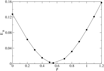
Figure 5: The binding energy $E_{B}$ with respect to single chain for a $32\times 33$ lattice as a function of $\rho=J_{d}/J_{\perp}$, $J_{\perp}=0.1$.

The above analysis is further supported by observing the evolution of the binding energy $E_{B}(L\times l)$ as a function of the number of chains in the lattice (Fig.  6). It clearly shows that when $J_{d}\approx 0.5J_{\perp}$, the binding energy is nearly independent of the number of chains and remains very close to that of the single chain. Hence it seems that at the point $J_{d}\approx 0.5J_{\perp}$, the ground state is made of independent chains as for $J_{\perp}=J_{d}=0$. This behavior is analogous to the domino model studied by Villain and coworkers villain , where a disordered ground state, made of independent chains for a particular value of the transverse coupling, was found.

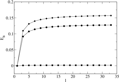
Figure 6: The binding energy $E_{B}$ with respect to single chain for a $32\times l$ lattice as a function of $l$ for $J_{d}/J_{\perp}=0$ (circles), $J_{d}/J_{\perp}=0.5$ (squares), $J_{d}/J_{\perp}=1.2$ (diamonds), $J_{\perp}=0.1$.

VII.2 Ground-state correlation functions

The behavior of the correlation functions is consistent with the existence of the three regimes found for the ground state energy. As expected, spin-spin correlations along the chains remain antiferromagnetic. The change of regimes will be detected by analyzing spin-spin correlations along the transverse direction. Fig. 7 shows the transverse magnetic structure factor $S_{\perp}(k_{\perp})$,

$$S_{\perp}(k_{\perp})=\sum_{k_{\perp}=1}^{L/2}{\bar{C}}_{\perp}(17,17,r)\cos k_{\perp}r$$ (49)

where $k_{\perp}$ is a wave number in the transverse direction. It also shows the three regimes discussed above. When $J_{d}\lesssim 0.5J_{\perp}$, $S_{\perp}(k_{\perp})$ has a maximum at $k_{\perp}=\pi$. The spin-spin correlations along the tranverse direction are AFM as for the longitudinal direction. For $J_{d}\approx 0.5J_{\perp}$, $S_{\perp}$ is structureless, a fact which is consistent with disconnected chains. When $J_{d}\gtrsim 0.5J_{\perp}$, $S_{\perp}$ has a maximum at $k_{\perp}=0$, and the correlations in the transverse direction are now ferromagnetic. This is the collinear magnetic state shown in Fig. 1.

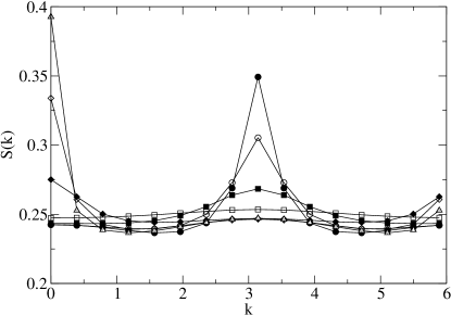
Figure 7: The ground state transverse structure factor for a $32\times 33$ lattice for $J_{d}/J_{\perp}=0$ (filled circles), $0.2$ (open circles), $0.4$ (filled squares), $0.55$ (open squares), $0.8$ (filled diamonds), $1.0$ (open diamonds), $1.2$ (open triangles).

The bond-strength ${\bar{C}}_{\perp}(17,17,1)$, computed in a $32\times 33$ lattice is shown in Fig. 8. It also shows that the chains seem to be disconnected when $J_{d}\approx 0.5J_{\perp}$. Starting from $J_{d}=0$, for which ${\bar{C}}_{\perp}(17,17,1)=-0.01846$, its absolute value first slowly decreases. Then, when $J_{d}$ is in the vicinity of $J_{d_{C}}$, the absolute value of ${\bar{C}}_{\perp}(17,17,1)$ sharply decreases and become very small; ${\bar{C}}_{\perp}(17,17,1)=-0.000799$ when $J_{d}=0.5J_{\perp}$. As soon as $J_{d}$ exceeds $J_{d_{C}}$, ${\bar{C}}_{\perp}(17,17,1)$ becomes ferromagnetic and starts to increase sharply. It later saturates when one is far enough from the critical point.

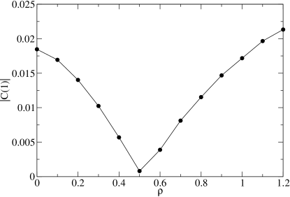
Figure 8: The bond-strength $C(1)={\bar{C}}_{\perp}(17,17,1)$ as a function of $\rho=J_{d}/J_{\perp}$, $J_{\perp}=0.1$.

VIII Long-range order in the ground state

The analysis made in the preceeding section indicates regions of dominant Néel or collinear spin-spin correlations or of a possibly disordered ground state at the transition point. But it does not tell if long range order is truly established. For this, it is necessary to look at the long-range behavior of the correlation functions.

The spurious effects due to the breaking of the translational symmetry, a consequence of the OBC, may be reduced by using a filter which smooths the action of the sites near the edges. In the results shown below in Fig  9, 10, 11, this was done as follows: ${\bar{C}}_{\parallel}(i,l,r)$ was first examined for a single chain for which the long distance behavior is known. Roughly, ${\bar{C}}_{\parallel}(i,l,r)\propto 1/r$ if logarithmic corrections are neglected. It was found that if the origin is taken at the middle of the chain, the $1/r$ behavior is roughly satisfied for $d\lesssim r\lesssim L/2-d$ with $d\approx 8$. The second inequality is due to edge effects. As a consequence, relatively large values of $L$ are necessary in order to observe the long range behavior, and lattices of up to $64\times 65$ were studied. The problem with such large lattices is that the energy width $\delta E(L)$ shrinks with increasing $L$ and the condition $\Delta_{\sigma}(L)\simeq J_{\perp,d}\ll\delta E(L)$ may not be fulfilled. For $L=64$, $ms_{1}=192$ and $ms_{2}=80$ states were kept. For these values, $\delta E(L=64)\approx 0.5$, which means $\delta E(L=64)/J_{\perp,d}\approx 5$ provided that $J_{\perp,d}\lesssim 0.16$.

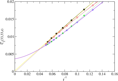
Figure 9: The ground state correlation function ${\bar{C}}_{\parallel}(33,33,r)$ for the $64\times 65$ lattice for $J_{\perp}=0$ (circles) and $J_{\perp}=0.16$ (squares). $J_{d}=0$ in both cases. The filled and open symbols correspond to odd and even distances respectively.

The first question which needs to be addressed is to know whether the DMRG can detect an eventual long range order. Comparisons with QMC for $L=32$ show that, the DMRG correlation in the transverse direction decays faster. This effect is expected to be larger on longer chains. But, despite this shortcoming of the method, one can still detect possible occurrence of long range order. If one considers the central chain in the 2D lattice, ${\bar{C}}_{\parallel}(L/2+1,L/2+1,r)$ is modified from that of an isolated chain because of the effective magnetic field created on it by the rest of lattice. Although this effective field is somewhat underevaluated by the DMRG because the transverse correlations are underevaluated, it can still be strong enough to lead to an ordered phase. This interpretation is related to the chain mean-field approach scalapino ; the essential point is that, here, no assumption about long-range order is made a priori. From this, one can see that if the DMRG method leads to a finite order parameter, it is necessarily genuine. Fig. 9 compares for the correlation function ${\bar{C}}_{\parallel}(33,33,r)$ for $J_{\perp}=0$, $J_{d}=0$ with $J_{\perp}=0.16$, $J_{d}=0$. In the first case when both transverse couplings are absent, ${\bar{C}}_{\parallel}(33,33,r)\propto 1/r$. The DMRG data still show an odd-even alternation, so fits must be perfomed for odd and even distances separately. The best least square fits to the data gave ${\bar{C}}_{\parallel}(33,33,r\rightarrow\infty)\approx 0.0001$. This is consistent with an absence of a long-range order for an isolated chain. But in the case $J_{\perp}=0.16$ and $J_{d}=0$, a fit to the data shows that ${\bar{C}}_{\parallel}(33,33,r)$ tends to ${\bar{C}}_{\parallel}(33,33,r\rightarrow\infty)\approx 0.0036$ The existence of long-range Néel order for $J_{\perp}=0.16$ is consistent with previous studies sandvik2 ; affleck . Adding $J_{\perp}$ alone seems to lead to long-range order. This has been recently shown in Ref.sandvik2 where values of $J_{\perp}$ down to $0.02$ were investigated. It is of course impossible to show from a numerical investigation whether any small value of $J_{\perp}$ will lead to an ordered state or there may be a disordered state for very small values of $J_{\perp}$. In view of current numerical results, the former hypothesis is more convincing.

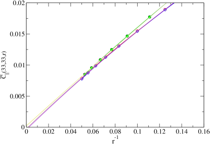
Figure 10: The ground state correlation function ${\bar{C}}_{\parallel}(33,33,r)$ for the $64\times 65$ lattice for $J_{\perp}=0.$, $J_{d}=0.$ (circles) and $J_{\perp}=0.16$, $J_{d}=0.08$ (squares). The filled and open symbols correspond to odd and even distances respectively.

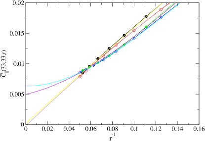
Figure 11: The ground state correlation function ${\bar{C}}_{\parallel}(33,33,r)$ for the $64\times 65$ lattice for $J_{\perp}=0.$, $J_{d}=0.$ (circles) and $J_{\perp}=0.16$, $J_{d}=0.16$ (squares). The filled and open symbols correspond to odd and even distances respectively.

The above discussion suggests that a frustration $J_{d}$ must be added in order to thwart the Néel state which results from the action of $J_{\perp}$. $J_{\perp}$ will now be set to $0.16$ and $J_{d}$ varied. For $J_{d}=0.08$, the value at which the analysis of smaller chains suggested that the ground state is made of disconnected chains, ${\bar{C}}_{\parallel}(33,33,r)$ is compared to the same quantity for a single chain in Fig. 10. Fits to the data show that the behavior of ${\bar{C}}_{\parallel}(33,33,r)$ is quite similar to that of a single chain. Clearly, for these values of the transverse couplings there is no long-range order in the ground state, and ${\bar{C}}_{\parallel}(33,33,r)$ seems to indicate that the ground state is made of a set of independent chains. It is important to emphasize that this result does not mean that the finite temperature effects are also trivial. The present situation could be similar to the so-called domino model first introduced by Andre andre and later studied by Villain and coworkers villain or to the crossed-chains quantum spin models singh . In the domino model, it was found that the ground state was made of disconnected chains but there was a long-range order at finite temperature. Indeed, the Mermin-Wagner theorem prohibits long-range order at finite temperatures for the 2D Heisenberg model. The finite temperature behavior in this case will thus be different.

The disconnected chain ground state is in contradiction with a recent study by Nersesyan and Tsvelik tsvelik . These authors argued, using bosonization, that when $J_{d}/J_{\perp}=0.5$, only the staggered part of the interchain part of the Hamiltonian vanishes. There remains a uniform part which is relevant and leads to two-dimensional spin liquid with a spin gap, $\Delta_{\sigma}\propto\exp(-\frac{\pi v_{\sigma}}{2J_{\perp}})$, where $v_{\sigma}$ is the spin velocity. The low energy excitations are argued to be unconfined spinons. The apparent contradiction between this conclusion and the numerical data above could be that the binding energies of the 2D spin liquid are very small, indeed $J_{\perp}=0.1$ corresponds to $\Delta_{\sigma}\approx 1.0\times 10^{-11}$. Such a small energy can obviously not be detected by a numerical method. A way to avoid this small energy scale is to raise $J_{\perp}$. This possibility is currently being investigated.

Finally, the collinear magnetic long range order is also confirmed by the analysis of ${\bar{C}}_{\parallel}(33,33,r)$. In Fig. 11, it is shown that for $J_{d}=0.1$, ${\bar{C}}_{\parallel}(33,33,r)$ converges even faster than for the Néel state above. The value of the extrapolated correlation is ${\bar{C}}_{\parallel}(33,33,r\rightarrow\infty)\approx 0.0056$.

IX Conclusions

In this paper, a new renormalization group method for weakly coupled chains was presented. It is based on solving numerically the model Hamiltonian in two 1D steps using the DMRG. During the first step, a low energy Hamiltonian for a single chain is obtained using the 1D DMRG. The original problem is then formulated as a perturbative expansion around the DMRG low energy Hamiltonian obtained during the first step. This perturbative expansion is a 1D problem which can also be solved by the DMRG.

The first and second order approximations were studied for weakly coupled Heisenberg chains with and without frustration. The results were compared to the QMC and showed good agreement for small systems and small transverse couplings. It was shown that, starting from the disordered 1D chain, the method can predict long-range order when it exists, a test generally failed by conventional perturbative methods. Calculations performed in the presence of frustration indicate an absence of a genuinely 2D spin liquid state. Instead, the frustration drives the Néel ground state to a collinear magnetic state. At the transition point, both ground-state energy and spin-spin correlation functions show a disordered ground state. The precise nature of this disordered ground state is currently under investigation.

The above results are very encouraging and indicate that the DMRG may become a very useful tool for the study of highly anisotropic 2D systems in the future. The method is only in its early stages, and some important improvements of the method are currently underway. These are the investigation of the role of cluster corrections, i.e., the starting point in the first step will be two-leg or three-leg ladders instead of a single chain; the use of exact diagonalization during the first step instead of DMRG. These improvements are likely to lead to better results for spin-spin correlations in the transverse direction. Extensions of the method to thermodynamic spin systems or fermionic models will also be made in the near future.

- (1) S. Moukouri and L.G. Caron, Phys. Rev. B 67, 092405 (2003).
- (2) S.R. White, Phys. Rev. Lett. 69, 2863 (1992). Phys. Rev. B 48, 10 345 (1993).
- (3) ’Density-Matrix Renormalization’, Ed. By I. Peschel, X. Wang, M. Kaulke and K. Hallberg, Springer (1998)
- (4) P.W. Anderson, Science 235, 1169 (1987).
- (5) P. Fazekas and P.W. Anderson, Philos. Mag. 30, 423 (1974).
- (6) P. Chandra and B. Douçot, Phys. Rev. B 38, 9335 (1988).
- (7) E. Dagotto and A. Moreo, Phys. Rev. Lett. 63, 2148 (1989).
- (8) P. Chandra, P. Coleman and A.I. Larkin, Phys. Rev. Lett. 64, 88 (1990).
- (9) L. Capriotti and S. Sorella, Phys. Rev. Lett. 84, 3173 (2000).
- (10) N. Read and S. Sachdev, Phys. Rev. Lett. 66, 1773 (1992).
- (11) A. Parola, S. Sorella and Q.F. Zhong, Phys. Rev. Lett. 71, 4393 (1993).
- (12) I. Affleck, M.P. Gelfand and R.R.P. Singh, J. Phys. A 27 7313 (1994); Erratum ibid. A 28, 1787 (1995).
- (13) H. Rosner et al., Phys. Rev. 56, 3402 (1997).
- (14) A.W. Sandvik, Phys. Rev. Lett. 83, 3069 (1999).
- (15) A.A. Nersesyan and A.M. Tsvelik, cond-mat/0206483.
- (16) S. K. Satija et al., Phys. Rev. B 21, 2001 (1980).
- (17) A. Keren et al., Phys. Rev. 48, 12926 (1993).
- (18) D. A. Tennant et al., Phys. Rev. B 52, 13381 (1995).
- (19) R. Coldea et al. Phys. Rev. Lett 86, 1335 (2001).
- (20) S. Moukouri physics/0312011.
- (21) T. Kato, Prog. Teor. Phys. 4, 514 (1949); 5, 95 (1950).
- (22) C. Bloch, Nucl. Phys. 6, 329 (1958).
- (23) A. Messiah ’Quantum Mechanics’, Ed. Dover, p. 685-720 (1999).
- (24) J.E. Hirsch and G.F. Mazenko, Phys. Rev. B 19, 2656 (1979).
- (25) O.A. Starykh, R.R.P. Singh and G.C. Levine, Phys. Rev. Lett. 88, 167203 (2002).
- (26) R. Mukhopadhyay, et al. Phys. Rev. B 64, 045120 (2001).
- (27) S. Moukouri and L.G. Caron, Phys. Rev. Lett. 77, 4640 (1996).
- (28) T. Sakai and M. Takahashi, J. Phys. Soc. Jpn. 58, 3131 (1989).
- (29) L.G. Caron and C. Bourbonnais, Phys. Rev. 66, 045101 (2002).
- (30) S.R. White and R.M. Noack, Phys. Rev. Lett. 68, 3487 (1992).
- (31) S.D. Drell, M. Weinstein and S. Yankielovicz, Phys. Rev. D 14, 487 (1976).
- (32) R. Jullien, P. Pfeuty, J.N. Fields and S. Doniach, Phys. Rev. B 18, 3568 (1978).
- (33) A.W. Sandvik and J. Kurkijärvi, Phys. Rev. B 43, 5950 (1991); A.W. Sandvik, Phys. Rev. B 59, 14157 (1999).
- (34) A.W. Sandvik and D.J. Scalapino, Phys. Rev. 47, 12333 (1993).
- (35) K. Hallberg, P. Horsch and G. Martinez, Phys. Rev. 52, 719 (1995).
- (36) D.J. Scalapino, Y. Imry, and P. Pincus, Phys. Rev. B 11, 2042 (1975).
- (37) J. Villain, R. Bidaux, J.-P. Carton and R. Conte, J. Physique 41, 1263 (1980).
- (38) G. André, R. Bidaux, R. Conte and L. de Seze, J. Physique 40, 479 (1979).