Momentum Distribution of a Weakly Coupled Fermi Gas

Girish S. Setlur The Institute of Mathematical Sciences
Taramani, Chennai 600113, India.
Abstract

We apply the sea-boson method to compute the momentum distribution of a spinless continuum Fermi gas in two space dimensions with short-range repulsive interactions. We find that the ground state of the system is a Landau Fermi liquid( $0<Z_{F}<1$ ). We also apply this method to study the one-dimensional system when the interactions are long-ranged gauge interactions. We map the Wigner crystal phase of this system.

I Introduction

In this article we apply the sea-boson method that is now powerful enough to yield most of the well-known results in one-dimension, to solve for the momentum distribution of electorns in the case when the electrons are in a continuum in two space dimensions with short range repulsive interactions. In other words, the two dimensional analog of the spinless Luttinger model. As a more nontrivial application we calculate the momentum distribution of a spinless Fermi system in one dimension with long-range confining (gauge) interactions and show that the system is a Wigner crystal. The momentum distribution of this system exhibits some unusual features that are probably new.

II The Hamiltonian

Here we compute the momentum distribution of the spinless Fermi gas with short-range repulsion in two space dimensions in an effort to ascertain whether or not this system describes a Landau Fermi liquid. This exercise is simple and is an alternative to studying the Hubbard model in 2d where the algebra is quite involved. We expect the answers to qualitative questions such as the validity of Fermi liquid theory to be the same in both models since both involve very short-range interactions. We have argued before that whenever Fermi liquid theory breaks down, it does so maximally. That is, it breaks down for all values of the coupling. Thus it is sufficient to study the weakly coupled 2D system with short-range interactions where the analysis is straightforward. The intuition gained from this can then be transplanted to the 2D Hubbard model at large $U$, which is likely to be hard to solve even using sea-bosons. On the other hand, there may some qualitatively new physics in the case of electrons with spin. This will become clearer when we actually decide to study the Hubbard model directly in future publications. In the present case, the hamiltonian in the sea-boson language is given by,

H=βˆ‘π€πͺ(𝐀.πͺm)​A𝐀†​(πͺ)​A𝐀​(πͺ)+βˆ‘πͺβ‰ 0vπͺ2​Vβ€‹βˆ‘π€π€β€²[A𝐀​(βˆ’πͺ)+A𝐀†​(πͺ)]​[A𝐀′​(πͺ)+A𝐀′†​(βˆ’πͺ)]𝐻subscript𝐀πͺformulae-sequence𝐀πͺπ‘šsubscriptsuperscript𝐴†𝐀πͺsubscript𝐴𝐀πͺsubscriptπͺ0subscript𝑣πͺ2𝑉subscriptsuperscript𝐀𝐀′delimited-[]subscript𝐴𝐀πͺsubscriptsuperscript𝐴†𝐀πͺdelimited-[]subscript𝐴superscript𝐀′πͺsubscriptsuperscript𝐴†superscript𝐀′πͺH=\sum_{{\bf{k}}{\bf{q}}}\left(\frac{{\bf{k.q}}}{m}\right)A^{\dagger}_{{\bf{k}}}({\bf{q}})A_{{\bf{k}}}({\bf{q}})+\sum_{{\bf{q}}\neq 0}\frac{v_{{\bf{q}}}}{2V}\sum_{{\bf{k}}{\bf{k}}^{{}^{\prime}}}[A_{{\bf{k}}}(-{\bf{q}})+A^{\dagger}_{{\bf{k}}}({\bf{q}})][A_{{\bf{k}}^{{}^{\prime}}}({\bf{q}})+A^{\dagger}_{{\bf{k}}^{{}^{\prime}}}(-{\bf{q}})] (1)

This hamiltonian describes a self-interacting Fermi gas provided we assume that $v_{{\bf{q}}}=\frac{v_{0}}{m}\mbox{ }\theta(\Lambda-|{\bf{q}}|)$ where $\Lambda\ll k_{F}$ here $0<v_{0}\ll 1$ is a dimensionless parameter. We may solve for the boson occupation number as follows.

$$\left<A^{\dagger}_{{\bf{k}}}({\bf{q}})A_{{\bf{k}}}({\bf{q}})\right>=\frac{1}{V}\sum_{i}\frac{\Lambda_{{\bf{k}}}(-{\bf{q}})}{(\omega_{i}+\frac{{\bf{k.q}}}{m})^{2}}g^{2}_{i}(-{\bf{q}})$$ (2)

where $\Lambda_{{\bf{k}}}(-{\bf{q}})=n_{F}({\bf{k}}-{\bf{q}}/2)(1-n_{F}({\bf{k}}+{\bf{q}}/2))$.

$$g^{-2}_{i}(-{\bf{q}})=\frac{1}{V}\mbox{ }\sum_{{\bf{k}}}\frac{n_{F}({\bf{k}}-{\bf{q}}/2)-n_{F}({\bf{k}}+{\bf{q}}/2)}{(\omega_{i}-\frac{{\bf{k.q}}}{m})^{2}}$$ (3)
$$\epsilon_{RPA}({\bf{q}},\omega)=1+\frac{v_{{\bf{q}}}}{V}\sum_{{\bf{k}}}\frac{n_{F}({\bf{k}}+{\bf{q}}/2)-n_{F}({\bf{k}}-{\bf{q}}/2)}{\omega-\frac{{\bf{k.q}}}{m}}$$ (4)

As argued in earlier works, we have to interpret sum over modes with care so as to not lose the particle-hole mode, the collective mode being obvious. The is particularly important in two dimensions where we expect both to be present. Thus the sum over modes is defined as follows.

$$\sum_{i}\mbox{ }f({\bf{q}},\omega_{i})=\frac{\int^{\infty}_{0}d\omega\mbox{ }W({\bf{q}},\omega)\mbox{ }f({\bf{q}},\omega)}{\int^{\infty}_{0}d\omega\mbox{ }W({\bf{q}},\omega)}$$ (5)

Here the weight function is given by,

$$W({\bf{q}},\omega)=-Im\left(\frac{1}{\epsilon_{RPA}({\bf{q}},\omega-i0^{+})}\right)$$ (6)

In our earlier work, we had suggested that in the above formula we have to use a dielectric function that is sensitive to significant qualitative changes in one-particle properties. The simple RPA dielectric function does not possess qualities we expect from a Wigner crystal. Thus we shall have to derive a new dielectric function using the localised basis rather than the plane-wave basis. In the case of the Fermi gas in two dimensions we find that the system is a Landau Fermi liquid and there is no need to use a better dielectric function, the simple RPA suffices. The momentum distirbution is always given by,

$$<n_{{\bf{k}}}>=\frac{1}{2}\left[1+e^{-2S^{0}_{B}({\bf{k}})}\right]\mbox{ }n_{F}({\bf{k}})+\frac{1}{2}\left[1-e^{-2S^{0}_{A}({\bf{k}})}\right]\mbox{ }(1-n_{F}({\bf{k}}))$$ (7)
$$S^{0}_{A}({\bf{k}})=\sum_{{\bf{q}}}\left<A^{\dagger}_{{\bf{k}}-{\bf{q}}/2}({\bf{q}})A_{{\bf{k}}-{\bf{q}}/2}({\bf{q}})\right>$$ (8)
$$S^{0}_{B}({\bf{k}})=\sum_{{\bf{q}}}\left<A^{\dagger}_{{\bf{k}}+{\bf{q}}/2}({\bf{q}})A_{{\bf{k}}+{\bf{q}}/2}({\bf{q}})\right>$$ (9)

The computation of the boson occupation number $\left<A^{\dagger}_{{\bf{k}}}({\bf{q}})A_{{\bf{k}}}({\bf{q}})\right>$ is the key to evaluating one-particle properties.

III The Computations

In this section, we compute the various quantities defined in the previous sections. In the case of a of a Fermi gas in two dimensions with short-range repulsive interactions we may use the simple RPA dielectric function. The integrals are somewhat complicated since in two dimensions, the angular parts are very troublesome unlike in three dimensions. Therefore we take the easy way out and copy the results first derived by Stern[1].

$$\epsilon^{r}_{RPA}(q,\omega)=1+\frac{mk_{F}v_{q}}{2\pi q}\{\frac{q}{k_{F}}-C_{-}\left[\left(\frac{q}{2k_{F}}-\frac{m\omega}{k_{F}q}\right)^{2}-1\right]^{\frac{1}{2}}-C_{+}\left[\left(\frac{q}{2k_{F}}+\frac{m\omega}{k_{F}q}\right)^{2}-1\right]^{\frac{1}{2}}\}$$ (10)
$$\epsilon^{i}_{RPA}(q,\omega)=\frac{mk_{F}v_{q}}{2\pi q}\{D_{-}\left[1-\left[\frac{q}{2k_{F}}-\frac{m\omega}{k_{F}q}\right]^{2}\right]^{\frac{1}{2}}-D_{+}\left[1-\left[\frac{q}{2k_{F}}+\frac{m\omega}{k_{F}q}\right]^{2}\right]^{\frac{1}{2}}\}$$ (11)

where,

$$C_{\pm}=sgn\left[\frac{q}{2k_{F}}\pm\frac{m\omega}{k_{F}q}\right],\mbox{ }D_{\pm}=0,\mbox{ }\left|\frac{q}{2k_{F}}\pm\frac{m\omega}{k_{F}q}\right|>1$$ (12)
$$C_{\pm}=0,\mbox{ }D_{\pm}=1,\mbox{ }\left|\frac{q}{2k_{F}}\pm\frac{m\omega}{k_{F}q}\right|<1$$ (13)
gβˆ’2​(βˆ’πͺ,Ο‰)=m​kF2​π​q​  ​{m​Cβˆ’kF​q​[(q2​kFβˆ’m​ωkF​q)2βˆ’1]βˆ’12​(q2​kFβˆ’m​ωkF​q)βˆ’m​C+kF​q​[(q2​kF+m​ωkF​q)2βˆ’1]βˆ’12​(q2​kF+m​ωkF​q)}superscript𝑔2πͺπœ”π‘šsubscriptπ‘˜πΉ2πœ‹π‘žΒ Β π‘šsubscript𝐢subscriptπ‘˜πΉπ‘žsuperscriptdelimited-[]superscriptπ‘ž2subscriptπ‘˜πΉπ‘šπœ”subscriptπ‘˜πΉπ‘ž2112π‘ž2subscriptπ‘˜πΉπ‘šπœ”subscriptπ‘˜πΉπ‘žπ‘šsubscript𝐢subscriptπ‘˜πΉπ‘žsuperscriptdelimited-[]superscriptπ‘ž2subscriptπ‘˜πΉπ‘šπœ”subscriptπ‘˜πΉπ‘ž2112π‘ž2subscriptπ‘˜πΉπ‘šπœ”subscriptπ‘˜πΉπ‘žg^{-2}(-{\bf{q}},\omega)=\frac{mk_{F}}{2\pi q}\mbox{ }\mbox{ }\{\frac{mC_{-}}{k_{F}q}\left[\left(\frac{q}{2k_{F}}-\frac{m\omega}{k_{F}q}\right)^{2}-1\right]^{-\frac{1}{2}}\left(\frac{q}{2k_{F}}-\frac{m\omega}{k_{F}q}\right)-\frac{mC_{+}}{k_{F}q}\left[\left(\frac{q}{2k_{F}}+\frac{m\omega}{k_{F}q}\right)^{2}-1\right]^{-\frac{1}{2}}\left(\frac{q}{2k_{F}}+\frac{m\omega}{k_{F}q}\right)\} (14)

$\displaystyle\left<A^{\dagger}_{{\bf{k}}}({\bf{q}})A_{{\bf{k}}}({\bf{q}})\right>=\frac{1}{V}\frac{1}{Z(q)}\int^{\infty}_{0}d\omega\mbox{ }W(q,\omega)\mbox{ }\frac{\Lambda_{{\bf{k}}}(-{\bf{q}})}{(\omega+\frac{{\bf{k.q}}}{m})^{2}}\mbox{ }g^{2}(-{\bf{q}},\omega)$

$$W(q,\omega)=\frac{\epsilon^{i}_{RPA}(q,\omega)}{\epsilon^{r2}_{RPA}(q,\omega)+\epsilon^{i2}_{RPA}(q,\omega)}$$ (15)
$$Z(q)=\int^{\infty}_{0}d\omega\mbox{ }W(q,\omega)$$ (16)

In general we have,

$$S^{0}_{A}({\bf{k}})=\frac{1}{(2\pi)^{2}}\int^{\infty}_{0}dq\mbox{ }q\mbox{ }\frac{1}{Z(q)}\int^{\infty}_{0}d\omega\mbox{ }W(q,\omega)\mbox{ }f_{A}(k,q,\omega)\mbox{ }g^{2}(-{\bf{q}},\omega)$$ (17)
$$S^{0}_{B}({\bf{k}})=\frac{1}{(2\pi)^{2}}\int^{\infty}_{0}dq\mbox{ }q\mbox{ }\frac{1}{Z(q)}\int^{\infty}_{0}d\omega\mbox{ }W(q,\omega)\mbox{ }f_{B}(k,q,\omega)g^{2}(-{\bf{q}},\omega)$$ (18)
fA​(k,q,Ο‰)=∫02​π𝑑θ​ ​θ​(kF2βˆ’k2βˆ’q2+2​k​q​c​o​s​(ΞΈ))(Ο‰+k​qm​c​o​s​(ΞΈ)βˆ’Ο΅q)2subscriptπ‘“π΄π‘˜π‘žπœ”subscriptsuperscript2πœ‹0differential-dπœƒΒ πœƒsuperscriptsubscriptπ‘˜πΉ2superscriptπ‘˜2superscriptπ‘ž22π‘˜π‘žπ‘π‘œπ‘ πœƒsuperscriptπœ”π‘˜π‘žπ‘šπ‘π‘œπ‘ πœƒsubscriptitalic-Ο΅π‘ž2f_{A}(k,q,\omega)=\int^{2\pi}_{0}d\theta\mbox{ }\frac{\theta(k_{F}^{2}-k^{2}-q^{2}+2kqcos(\theta))}{(\omega+\frac{kq}{m}cos(\theta)-\epsilon_{q})^{2}} (19)
fB​(k,q,Ο‰)=∫02​π𝑑θ​ ​θ​(k2+q2βˆ’kF2+2​k​q​c​o​s​(ΞΈ))(Ο‰+k​qm​c​o​s​(ΞΈ)+Ο΅q)2subscriptπ‘“π΅π‘˜π‘žπœ”subscriptsuperscript2πœ‹0differential-dπœƒΒ πœƒsuperscriptπ‘˜2superscriptπ‘ž2superscriptsubscriptπ‘˜πΉ22π‘˜π‘žπ‘π‘œπ‘ πœƒsuperscriptπœ”π‘˜π‘žπ‘šπ‘π‘œπ‘ πœƒsubscriptitalic-Ο΅π‘ž2f_{B}(k,q,\omega)=\int^{2\pi}_{0}d\theta\mbox{ }\frac{\theta(k^{2}+q^{2}-k_{F}^{2}+2kqcos(\theta))}{(\omega+\frac{kq}{m}cos(\theta)+\epsilon_{q})^{2}} (20)

Define,

u​(x;A,B)β‰‘βˆ«π‘‘x​ ​1(A+B​ ​C​o​s​[x])2𝑒π‘₯𝐴𝐡differential-dπ‘₯Β 1superscriptπ΄π΅Β πΆπ‘œπ‘ delimited-[]π‘₯2u(x;A,B)\equiv\int dx\mbox{ }\frac{1}{(A+B\mbox{ }Cos[x])^{2}} (21)

From $Mathematica^{TM}$ we find,


$\displaystyle u(x;A,B)=-2A\frac{\mbox{ }ArcTanh\left[\frac{(A-B)Tan\left[\frac{x}{2}\right]}{\sqrt{B^{2}-A^{2}}}\right]}{(A^{2}-B^{2})\sqrt{B^{2}-A^{2}}}$

+B​ ​S​i​n​[x](B2βˆ’A2)​(A+B​ ​C​o​s​[x])𝐡 𝑆𝑖𝑛delimited-[]π‘₯superscript𝐡2superscript𝐴2π΄π΅Β πΆπ‘œπ‘ delimited-[]π‘₯+\frac{B\mbox{ }Sin[x]}{(B^{2}-A^{2})(A+B\mbox{ }Cos[x])} (22)

Integrating by parts we find,

fA​(k,q,Ο‰)=∫02​π𝑑θ​ ​s​i​n​θ​  ​δ​(kF2βˆ’k2βˆ’q22​k​q+c​o​s​(ΞΈ))​ ​u​(ΞΈ;Ο‰βˆ’Ο΅q,k​qm)subscriptπ‘“π΄π‘˜π‘žπœ”subscriptsuperscript2πœ‹0differential-dπœƒΒ π‘ π‘–π‘›πœƒΒ Β π›Ώsuperscriptsubscriptπ‘˜πΉ2superscriptπ‘˜2superscriptπ‘ž22π‘˜π‘žπ‘π‘œπ‘ πœƒΒ π‘’πœƒπœ”subscriptitalic-Ο΅π‘žπ‘˜π‘žπ‘šf_{A}(k,q,\omega)=\int^{2\pi}_{0}d\theta\mbox{ }sin\theta\mbox{ }\mbox{ }\delta(\frac{k_{F}^{2}-k^{2}-q^{2}}{2kq}+cos(\theta))\mbox{ }u(\theta;\omega-\epsilon_{q},\frac{kq}{m}) (23)
fB​(k,q,Ο‰)=∫02​π𝑑θ​ ​s​i​n​θ​  ​δ​(k2+q2βˆ’kF22​k​q+c​o​s​(ΞΈ))​ ​u​(ΞΈ;Ο‰+Ο΅q,k​qm)subscriptπ‘“π΅π‘˜π‘žπœ”subscriptsuperscript2πœ‹0differential-dπœƒΒ π‘ π‘–π‘›πœƒΒ Β π›Ώsuperscriptπ‘˜2superscriptπ‘ž2superscriptsubscriptπ‘˜πΉ22π‘˜π‘žπ‘π‘œπ‘ πœƒΒ π‘’πœƒπœ”subscriptitalic-Ο΅π‘žπ‘˜π‘žπ‘šf_{B}(k,q,\omega)=\int^{2\pi}_{0}d\theta\mbox{ }sin\theta\mbox{ }\mbox{ }\delta(\frac{k^{2}+q^{2}-k_{F}^{2}}{2kq}+cos(\theta))\mbox{ }u(\theta;\omega+\epsilon_{q},\frac{kq}{m}) (24)

This may be rewritten as,


fA​(k,q,Ο‰)=∫0π𝑑θ​ ​s​i​n​θ​  ​δ​(kF2βˆ’k2βˆ’q22​k​q+c​o​s​(ΞΈ))​ ​u​(ΞΈ;Ο‰βˆ’Ο΅q,k​qm)subscriptπ‘“π΄π‘˜π‘žπœ”subscriptsuperscriptπœ‹0differential-dπœƒΒ π‘ π‘–π‘›πœƒΒ Β π›Ώsuperscriptsubscriptπ‘˜πΉ2superscriptπ‘˜2superscriptπ‘ž22π‘˜π‘žπ‘π‘œπ‘ πœƒΒ π‘’πœƒπœ”subscriptitalic-Ο΅π‘žπ‘˜π‘žπ‘š\displaystyle f_{A}(k,q,\omega)=\int^{\pi}_{0}d\theta\mbox{ }sin\theta\mbox{ }\mbox{ }\delta(\frac{k_{F}^{2}-k^{2}-q^{2}}{2kq}+cos(\theta))\mbox{ }u(\theta;\omega-\epsilon_{q},\frac{kq}{m})

βˆ’βˆ«0π𝑑θ​ ​s​i​n​θ​  ​δ​(kF2βˆ’k2βˆ’q22​k​qβˆ’c​o​s​(ΞΈ))​ ​u​(ΞΈ+Ο€;Ο‰βˆ’Ο΅q,k​qm)subscriptsuperscriptπœ‹0differential-dπœƒΒ π‘ π‘–π‘›πœƒΒ Β π›Ώsuperscriptsubscriptπ‘˜πΉ2superscriptπ‘˜2superscriptπ‘ž22π‘˜π‘žπ‘π‘œπ‘ πœƒΒ π‘’πœƒπœ‹πœ”subscriptitalic-Ο΅π‘žπ‘˜π‘žπ‘š-\int^{\pi}_{0}d\theta\mbox{ }sin\theta\mbox{ }\mbox{ }\delta(\frac{k_{F}^{2}-k^{2}-q^{2}}{2kq}-cos(\theta))\mbox{ }u(\theta+\pi;\omega-\epsilon_{q},\frac{kq}{m}) (25)

fB​(k,q,Ο‰)=∫0π𝑑θ​ ​s​i​n​θ​  ​δ​(k2+q2βˆ’kF22​k​q+c​o​s​(ΞΈ))​ ​u​(ΞΈ;Ο‰+Ο΅q,k​qm)subscriptπ‘“π΅π‘˜π‘žπœ”subscriptsuperscriptπœ‹0differential-dπœƒΒ π‘ π‘–π‘›πœƒΒ Β π›Ώsuperscriptπ‘˜2superscriptπ‘ž2superscriptsubscriptπ‘˜πΉ22π‘˜π‘žπ‘π‘œπ‘ πœƒΒ π‘’πœƒπœ”subscriptitalic-Ο΅π‘žπ‘˜π‘žπ‘š\displaystyle f_{B}(k,q,\omega)=\int^{\pi}_{0}d\theta\mbox{ }sin\theta\mbox{ }\mbox{ }\delta(\frac{k^{2}+q^{2}-k_{F}^{2}}{2kq}+cos(\theta))\mbox{ }u(\theta;\omega+\epsilon_{q},\frac{kq}{m})

βˆ’βˆ«0π𝑑θ​ ​s​i​n​θ​  ​δ​(k2+q2βˆ’kF22​k​qβˆ’c​o​s​(ΞΈ))​ ​u​(ΞΈ+Ο€;Ο‰+Ο΅q,k​qm)subscriptsuperscriptπœ‹0differential-dπœƒΒ π‘ π‘–π‘›πœƒΒ Β π›Ώsuperscriptπ‘˜2superscriptπ‘ž2superscriptsubscriptπ‘˜πΉ22π‘˜π‘žπ‘π‘œπ‘ πœƒΒ π‘’πœƒπœ‹πœ”subscriptitalic-Ο΅π‘žπ‘˜π‘žπ‘š-\int^{\pi}_{0}d\theta\mbox{ }sin\theta\mbox{ }\mbox{ }\delta(\frac{k^{2}+q^{2}-k_{F}^{2}}{2kq}-cos(\theta))\mbox{ }u(\theta+\pi;\omega+\epsilon_{q},\frac{kq}{m}) (26)
ΞΈ0=a​r​c​c​o​s​[k2+q2βˆ’kF22​k​q]subscriptπœƒ0π‘Žπ‘Ÿπ‘π‘π‘œπ‘ delimited-[]superscriptπ‘˜2superscriptπ‘ž2superscriptsubscriptπ‘˜πΉ22π‘˜π‘ž\theta_{0}=arccos\left[\frac{k^{2}+q^{2}-k_{F}^{2}}{2kq}\right] (27)
ΞΈ0β€²=a​r​c​c​o​s​[βˆ’k2βˆ’q2+kF22​k​q]subscriptsuperscriptπœƒβ€²0π‘Žπ‘Ÿπ‘π‘π‘œπ‘ delimited-[]superscriptπ‘˜2superscriptπ‘ž2superscriptsubscriptπ‘˜πΉ22π‘˜π‘ž\theta^{{}^{\prime}}_{0}=arccos\left[\frac{-k^{2}-q^{2}+k_{F}^{2}}{2kq}\right] (28)

$\displaystyle f_{A}(k,q,\omega)=u(\theta_{0};\omega-\epsilon_{q},\frac{kq}{m})\left[\theta(\frac{k_{F}^{2}-k^{2}-q^{2}}{2kq}+1)-\theta(\frac{k_{F}^{2}-k^{2}-q^{2}}{2kq}-1)\right]$

$$-u(\theta^{{}^{\prime}}_{0}+\pi;\omega-\epsilon_{q},\frac{kq}{m})\left[\theta(1-\frac{k_{F}^{2}-k^{2}-q^{2}}{2kq})-\theta(-1-\frac{k_{F}^{2}-k^{2}-q^{2}}{2kq})\right]$$ (29)

$\displaystyle f_{B}(k,q,\omega)=u(\theta^{{}^{\prime}}_{0};\omega+\epsilon_{q},\frac{kq}{m})\left[\theta(\frac{k^{2}+q^{2}-k_{F}^{2}}{2kq}+1)-\theta(\frac{k^{2}+q^{2}-k_{F}^{2}}{2kq}-1)\right]$

$$-u(\theta_{0}+\pi;\omega+\epsilon_{q},\frac{kq}{m})\mbox{ }\left[\theta(1-\frac{k^{2}+q^{2}-k_{F}^{2}}{2kq})-\theta(-1-\frac{k^{2}+q^{2}-k_{F}^{2}}{2kq})\right]$$ (30)

The collective mode occurs when $Im[\epsilon]=0$, that is, for small enough $q$. This means that we have to treat this separately.


$\displaystyle S^{0}_{A}({\bf{k}})=\frac{1}{(2\pi)^{2}}\int^{\infty}_{0}dq\mbox{ }q\mbox{ }\frac{1}{Z(q)}\int^{\infty}_{0}d\omega\mbox{ }W(q,\omega)\mbox{ }f_{A}(k,q,\omega)\mbox{ }g^{2}(-{\bf{q}},\omega)$

+1(2​π)2β€‹βˆ«0βˆžπ‘‘q​ ​q​  ​fA​(k,q,Ο‰c)​ ​g2​(βˆ’πͺ,Ο‰c)1superscript2πœ‹2subscriptsuperscript0differential-dπ‘žΒ π‘žΒ Β subscriptπ‘“π΄π‘˜π‘žsubscriptπœ”π‘Β superscript𝑔2πͺsubscriptπœ”π‘+\frac{1}{(2\pi)^{2}}\int^{\infty}_{0}dq\mbox{ }q\mbox{ }\mbox{ }f_{A}(k,q,\omega_{c})\mbox{ }g^{2}(-{\bf{q}},\omega_{c}) (31)

$\displaystyle S^{0}_{B}({\bf{k}})=\frac{1}{(2\pi)^{2}}\int^{\infty}_{0}dq\mbox{ }q\mbox{ }\frac{1}{Z(q)}\int^{\infty}_{0}d\omega\mbox{ }W(q,\omega)\mbox{ }f_{B}(k,q,\omega)g^{2}(-{\bf{q}},\omega)$

$$+\frac{1}{(2\pi)^{2}}\int^{\infty}_{0}dq\mbox{ }q\mbox{ }f_{B}(k,q,\omega_{c})g^{2}(-{\bf{q}},\omega_{c})$$ (32)

Here it is implicit that in $W$ we assume that I​m​[Ο΅]β‰ 0πΌπ‘šdelimited-[]italic-Ο΅0Im[\epsilon]\neq 0. The dispersion of the collective mode may be found using ${\it{Mathematica}}^{TM}$. It is given below.

$$\omega_{c}(q)=q\mbox{ }(2\pi+mv_{q})\frac{(\pi^{2}q^{2}+m\pi q^{2}v_{q}+k_{F}^{2}m^{2}v_{q}^{2})^{\frac{1}{2}}}{2m^{2}\sqrt{\pi}v_{q}\sqrt{\pi+mv_{q}}}$$ (33)

This dispersion is real and positive for all $q$ and for all $v_{q}>0$. Thus in the small $q$ limit, where using just the RPA dielectric function is justified and is also the limit where the close to the Fermi surface features of the momentum distribution is given exactly, we are justified in retaining only the coherent part. Thus we may write,

SA0​(𝐀)β‰ˆ1(2​π)2β€‹βˆ«0βˆžπ‘‘q​ ​q​  ​fA​(k,q,Ο‰c)​ ​g2​(βˆ’πͺ,Ο‰c)subscriptsuperscript𝑆0𝐴𝐀1superscript2πœ‹2subscriptsuperscript0differential-dπ‘žΒ π‘žΒ Β subscriptπ‘“π΄π‘˜π‘žsubscriptπœ”π‘Β superscript𝑔2πͺsubscriptπœ”π‘S^{0}_{A}({\bf{k}})\approx\frac{1}{(2\pi)^{2}}\int^{\infty}_{0}dq\mbox{ }q\mbox{ }\mbox{ }f_{A}(k,q,\omega_{c})\mbox{ }g^{2}(-{\bf{q}},\omega_{c}) (34)
$$S^{0}_{B}({\bf{k}})\approx\frac{1}{(2\pi)^{2}}\int^{\infty}_{0}dq\mbox{ }q\mbox{ }f_{B}(k,q,\omega_{c})g^{2}(-{\bf{q}},\omega_{c})$$ (35)

To determine whether or not Fermi liquid theory breaks down, we have to compute,

SA0​(kF)β‰ˆ1(2​π)2β€‹βˆ«0βˆžπ‘‘q​ ​q​  ​fA​(kF,q,Ο‰c)​ ​g2​(βˆ’πͺ,Ο‰c)subscriptsuperscript𝑆0𝐴subscriptπ‘˜πΉ1superscript2πœ‹2subscriptsuperscript0differential-dπ‘žΒ π‘žΒ Β subscript𝑓𝐴subscriptπ‘˜πΉπ‘žsubscriptπœ”π‘Β superscript𝑔2πͺsubscriptπœ”π‘S^{0}_{A}(k_{F})\approx\frac{1}{(2\pi)^{2}}\int^{\infty}_{0}dq\mbox{ }q\mbox{ }\mbox{ }f_{A}(k_{F},q,\omega_{c})\mbox{ }g^{2}(-{\bf{q}},\omega_{c}) (36)
$$S^{0}_{B}(k_{F})\approx\frac{1}{(2\pi)^{2}}\int^{\infty}_{0}dq\mbox{ }q\mbox{ }f_{B}(k_{F},q,\omega_{c})g^{2}(-{\bf{q}},\omega_{c})$$ (37)

If $S^{0}_{A}(k_{F}),S^{0}_{B}(k_{F})<\infty$ then the ground state is a Landau Fermi liquid. If $S^{0}_{A}(k_{F})=S^{0}_{B}(k_{F})=\infty$ then the system is a non-Fermi liquid. For small $q$ if we set $\omega_{c}=v_{eff}\mbox{ }q$ we have,

$$f_{A}(k_{F},q,\omega_{c})\sim f_{B}(k_{F},q,\omega_{c})\sim 1/q^{2}$$ (38)

Also,

$$g^{2}(-{\bf{q}},\omega_{c})\sim q$$ (39)

Thus the integrals in Eq.(Β 36) and Eq.(Β 37) are infrared finite. This means that $S^{0}_{A}(k_{F}),S^{0}_{B}(k_{F})<\infty$ and the system is a Landau Fermi liquid. The details of the momentum distribution can be worked out but are not terribly important.

IV One Dimensional System with Long-Range Interactions

In this case, we expect the system to be a Wigner crystal. Thus we have to be careful about the choice of the dielectric function. First, we postulate that $v_{q}=2e^{2}/(q\mbox{ }a)^{2}$ which corresponds to the gauge potential. Here $a$ has dimensions of length and $e^{2}>0$ is dimensionless. From the form of this potential, one hopes that we need not concern ourselves with the issues that were relevant in the case of the Calogero-Sutherland model namely the repulsion attraction duality (more prosaically called back-scattering). Thus we may write as before,


$\displaystyle\left<A^{\dagger}_{{\bf{k}}}({\bf{q}})A_{{\bf{k}}}({\bf{q}})\right>=\frac{1}{V}\frac{1}{Z(q)}\int^{\infty}_{0}d\omega\mbox{ }W(q,\omega)\mbox{ }\frac{\Lambda_{{\bf{k}}}(-{\bf{q}})}{(\omega+\frac{{\bf{k.q}}}{m})^{2}}\mbox{ }g^{2}(-{\bf{q}},\omega)$

$$W(q,\omega)=\frac{\epsilon^{i}(q,\omega)}{\epsilon^{r2}(q,\omega)+\epsilon^{i2}(q,\omega)}$$ (40)
$$Z(q)=\int^{\infty}_{0}d\omega\mbox{ }W(q,\omega)$$ (41)
$$g^{-2}(-{\bf{q}},\omega)=\frac{1}{v_{q}}\frac{\partial}{\partial\omega}\epsilon({\bf{q}},\omega)$$ (42)

As mentioned before, we have to be extra careful in making sure that we choose the right dielectric function. The RPA-dielectric function is not likely to suffice since its static structure factor (SSF) does not exhibit the features we expect from a Wigner crystal. In particular, we expect $S(2k_{F})=\infty$ as we shall see soon. To convince ourselves of this we ascertain the properties of the RPA dielectric function with long-range interactions.

$$\epsilon^{r}_{RPA}(q,\omega)=1+v_{q}\frac{m}{2\pi q}Log\left[\frac{(k_{F}+q/2)^{2}-\left(\frac{m\omega}{q}\right)^{2}}{(k_{F}-q/2)^{2}-\left(\frac{m\omega}{q}\right)^{2}}\right]$$ (43)

The zero of the above dielectric function gives us the dispersion of the collective modes.

$$\omega_{c}(q)=\frac{|q|}{m}\sqrt{\frac{(k_{F}+q/2)^{2}-(k_{F}-q/2)^{2}exp(-\frac{2\pi q}{mv_{q}})}{1-exp(-\frac{2\pi q}{mv_{q}})}}$$ (44)

For $|q|\ll k_{F}$ and $v_{q}=2e^{2}/(aq)^{2}$ we find,

$$\omega_{c}(q)\approx\frac{1}{m}\sqrt{\frac{e^{2}k_{F}m}{a^{2}}}\sqrt{\frac{2}{\pi}}+\frac{a^{2}k_{F}\sqrt{\frac{e^{2}k_{F}m}{a^{2}}}\sqrt{\frac{\pi}{2}}q^{2}}{2e^{2}m^{2}}+O(q^{4})$$ (45)

This plasmon-like gap $\omega_{0}\equiv\frac{1}{m}\sqrt{\frac{e^{2}k_{F}m}{a^{2}}}\sqrt{\frac{2}{\pi}}$ in the collective mode is present due to the characteristic $1/q^{2}$ nature of the potential. But this is also present in the three dimensional electron gas and is not a sign of an insulator since the latter is not at high densities. A gap in the one-particle Green function at the Fermi momentum could be taken as a sign of insulating behaviour[3]. However, in our approach we are unable to compute the full Green function as yet. Thus we must resort to a more indirect approach. For a Wigner crystal, the SSF must exhibit certain singularities. Thus we have to use the generalised-RPA that is sensitive to qualitative changes in single-particle properties. The new dielectric function will involve the full momentum distribution which has to be determined self-consistently using the above sea-boson equations. In our earlier work we suggested that the new dielectric function should also involve fluctutations in the momentum distribution, however it now appears that that is fortunately not needed. The number-number correlation function is vanishingly small in the thermodynamic limit as shown in another preprint and this means we may simply write,

$$\epsilon({\bf{q}},\omega)=1+\frac{v_{q}}{L}\sum_{k}\frac{{\bar{n}}_{k+q/2}-{\bar{n}}_{k-q/2}}{\omega-\xi_{k+q/2}+\xi_{k-q/2}}$$ (46)
ΞΎk=k22​mβˆ’βˆ‘qβ‰ 0vqL​nΒ―kβˆ’qsubscriptπœ‰π‘˜superscriptπ‘˜22π‘šsubscriptπ‘ž0subscriptπ‘£π‘žπΏsubscriptΒ―π‘›π‘˜π‘ž\xi_{k}=\frac{k^{2}}{2m}-\sum_{q\neq 0}\frac{v_{q}}{L}{\bar{n}}_{k-q} (47)

and the momentum distribution is determined self-consistently using the sea-boson equations (Eq.(Β 7)). This is too difficult to solve analytically and hence we have to resort to a numerical solution. In order to simplify proceedings even further, we use only the collective mode. The particle-hole mode which is due to a nonzero $Im[\epsilon]$ is needed if one is interested in features of the momentum distribution away from the Fermi surface more accurately. However we shall hope that this is given not too badly even at these regions far from the Fermi points.

$$\left<A^{\dagger}_{{\bf{k}}}({\bf{q}})A_{{\bf{k}}}({\bf{q}})\right>=\frac{1}{V}\mbox{ }\frac{\Lambda_{{\bf{k}}}(-{\bf{q}})}{(\omega_{c}(q)+\frac{k.q}{m})^{2}}\mbox{ }g^{2}(-{\bf{q}},\omega_{c})$$ (48)
$$g^{-2}(-{\bf{q}},\omega_{c})=\frac{m\omega_{c}}{\pi q}\left[\frac{1}{\omega_{c}^{2}-(v_{F}q+\epsilon_{q})^{2}}-\frac{1}{\omega_{c}^{2}-(v_{F}q-\epsilon_{q})^{2}}\right]$$ (49)
$$S^{0}_{A}(k)=\frac{1}{L}\sum_{q}\mbox{ }\frac{n_{F}(k-q)}{(\omega_{c}(q)+\frac{k.q}{m}-\epsilon_{q})^{2}}\mbox{ }g^{2}(-{\bf{q}},\omega_{c})$$ (50)
$$S^{0}_{B}(k)=\frac{1}{L}\sum_{q}\mbox{ }\frac{(1-n_{F}(k+q))}{(\omega_{c}(q)+\frac{k.q}{m}+\epsilon_{q})^{2}}\mbox{ }g^{2}(-{\bf{q}},\omega_{c})$$ (51)

To proceed further, we have to ascertain the nature of the collective modes $\omega_{c}$. If we use the RPA-dielectric function, we find a constant dispersion (plasmon) for small $|q|$. However we have found that this choice is inconsistent since if we use the momentum distribution obtained from this to solve for the dielectric function and recompute the collective mode we obtain a completely different answer namely : Ο‰c​(q)=vs​|q|subscriptπœ”π‘π‘žsubscriptπ‘£π‘ π‘ž\omega_{c}(q)=v_{s}|q|. Therefore it is critical that we get the dispersion right. It appears then that we have to use the form given in the appendix which is not easy to simplify. A systematic approach for obtaining the dispersion of the collective modes has been suggested by Sen and Baskaran[5]. Since the plane-wave basis is not appropriate for deriving a formula for the dielectric function of a Wigner crystal, we shall follow this approach. First, we would like ascertain the lattice structure in the small $a$ limit. In this limit, the potential energy dominates over the kinetic energy. If we assume that the electrons are all on a circle of perimeter $L$ then to minimise the potential energy, we have to maximize the separation. This leads to an equally spaced set of lattice points with lattice constant $l_{c}$ such that $N\mbox{ }l_{c}=L$. Thus we have $l_{c}=1/\rho_{0}=\pi/k_{F}$. Thus we assume that the electrons all lie on a circle with equal spacing between them. Therefore we expect the structure factor to diverge for a momentum $q_{0}=2\pi/l_{c}=2k_{F}$. From the Bijl-Feynman formula $S(q)=\epsilon_{q}/\omega_{c}(q)$ we may suspect that a choice of $\omega_{c}$ that vanishes at $q=2k_{F}$ is needed. The form of the dispersion is given in the appendix. For $\pi/N\ll|q\mbox{ }l_{c}|\ll 2\pi$ it seems that $\omega_{q}\approx\omega_{0}$. For $|q\mbox{ }l_{c}|\ll\pi/N$ we have to be more careful. And of course we must have $\omega_{q}=0$ for $q\mbox{ }l_{c}=\pm 2\pi$. But since in the thermodynamic limit $\pi/N\approx 0$ we may choose (hopefully) $\omega_{q}\approx\omega_{0}$. In Fig. 1 and 2 we see the momentum distribution obtained from these formulas has been plotted. In fact, we may write down a closed formula for the momentum distribution.

$${\bar{n}}_{k}=\frac{1}{2}(1+Exp\left[-\frac{m\mbox{ }\omega_{0}}{k_{F}^{2}-k^{2}}\right])n_{F}(k)+\frac{1}{2}(1-Exp\left[-\frac{m\mbox{ }\omega_{0}}{k^{2}-k_{F}^{2}}\right])(1-n_{F}(k))$$ (52)

The striking feature of this momentum distribution is that it is perfectly flat at $|k|=k_{F}$. In other words, not only is the slope zero but all the derivatives of the momentum distribution vanish at $|k|=k_{F}$. This is a striking prediction. This may be contrasted with the smooth Gaussian function of Gori-Giorgi and Ziesche [2]( Eq.(B1) in their Appendix B ). But they consider three dimensional systems which may be different from the one studied here. One particle spectral functions are accessible to tunneling experiments or angle-resolved photoemission spectroscopy(ARPES). A more difficult problem may be to experimentally realise a 1d electron system with long-range gauge interactions.

Refer to caption

FIG. 1.: Momentum Distribution of a Wigner Crystal (with zoom)

Refer to caption

FIG. 2.: Momentum Distribution of a Wigner Crystal (no zoom)

The formula below for the static structure factor is derived in the appendix.

$$S(q)=\frac{1}{N}\mbox{ }\frac{sin^{2}(\frac{qN\mbox{ }l_{c}}{2})}{sin^{2}(\frac{q\mbox{ }l_{c}}{2})}\mbox{ }e^{-\frac{q^{2}}{m\omega_{0}}}$$ (53)

This may be further simplified in the thermodynamic limit as follows. Consider,

$$\delta(x)\approx\frac{sin(N\mbox{ }x)}{\pi\mbox{ }x}$$ (54)

Then we may write,

$$S(q)=\delta(q)\frac{2\pi}{l_{c}}+\delta(q-2k_{F})\frac{2\pi}{l_{c}}\mbox{ }e^{-\frac{4k_{F}^{2}}{m\omega_{0}}}$$ (55)

As we can see here the strucutre factor diverges at $|q|=2k_{F}$ which means the system is a Wigner crystal ( a true Wigner crystal, since the divergence is from a delta-function )

V Appendix

Here we use the approach suggested by Sen[5] to derive a formula for the collective modes. The formula Eq.(Β 46) although probably right is not very illuminating, for it is hard to see how the structure factor derived from this formula possesses the features we expect namely a divergence at $|q|=2k_{F}$. Thus we would like to derive a formula for the dielectric function where this feature is manifest. To do this we adopt the localised basis rather than the plane-wave basis. In real space, the hamiltonian we are studying is written as follows.

$$H=\sum_{i=0}^{N-1}\frac{p^{2}_{i}}{2m}-\frac{e^{2}}{a^{2}}\sum_{i>j}|x_{i}-x_{j}|$$ (56)

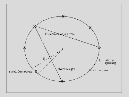
We assume that particles are on a circle and $|x|$ is the chord length. We would like to compute the dielectric function using this model. The density operator in momentum space is,

$$\rho_{{\bf{q}}}=\sum_{m=0}^{N-1}e^{iq\left(m\mbox{ }l_{c}+{\tilde{x}}_{m}\right)}$$ (57)

Here $x_{m}=m\mbox{ }l_{c}+{\tilde{x}}_{m}$ is measured along the circumference of the circle (see Fig. 3 below).

Refer to caption

FIG. 3.: Schematic Diagram of Electrons on a Circular Lattice

The average density is given by,

$$\left<\rho_{{\bf{q}}}\right>=\sum_{m=0}^{N-1}e^{iq\mbox{ }m\mbox{ }l_{c}}e^{-\frac{1}{2}q^{2}\mbox{ }<{\tilde{x}}^{2}_{m}>}$$ (58)

It can be shown that (see below) $<{\tilde{x}}^{2}_{n}>=1/m\omega_{0}$, independent of the index $n$. Thus we have,

$$\left<\rho_{{\bf{q}}}\right>=\frac{1-e^{iqN\mbox{ }l_{c}}}{1-e^{iq\mbox{ }l_{c}}}e^{-\frac{q^{2}}{2m\omega_{0}}}$$ (59)

In those instances where <ρq>β‰ 0expectationsubscriptπœŒπ‘ž0<\rho_{q}>\neq 0 the static structure factor is given by,

$$S(q)\equiv\frac{|<\rho_{{\bf{q}}}>|^{2}}{N}=\frac{1}{N}\mbox{ }\left(\vline\frac{1-e^{iqN\mbox{ }l_{c}}}{1-e^{iq\mbox{ }l_{c}}}\vline\right)^{2}\mbox{ }e^{-\frac{q^{2}}{m\omega_{0}}}=\frac{1}{N}\mbox{ }\frac{sin^{2}(\frac{qN\mbox{ }l_{c}}{2})}{sin^{2}(\frac{q\mbox{ }l_{c}}{2})}\mbox{ }e^{-\frac{q^{2}}{m\omega_{0}}}$$ (60)

The rest of the details are as follows. We write ${\tilde{x}}_{m}(t)\approx R\mbox{ }{\tilde{\theta}}_{m}(t)$. In terms of the small angles ${\tilde{\theta}}_{i}$ the hamiltonian in Eq.(Β 56) may be written as follows.

H=βˆ’12​m​R2β€‹βˆ‘m=0Nβˆ’1Β β€‹βˆ‚2βˆ‚ΞΈ~m2βˆ’R​ ​e22​a2β€‹βˆ‘mβ‰ mβ€²[(c​o​s​(2​π​mN+ΞΈ~m)βˆ’c​o​s​(2​π​mβ€²N+ΞΈ~mβ€²))2+(s​i​n​(2​π​mN+ΞΈ~m)βˆ’s​i​n​(2​π​mβ€²N+ΞΈ~mβ€²))2]12𝐻12π‘šsuperscript𝑅2superscriptsubscriptπ‘š0𝑁1Β superscript2subscriptsuperscript~πœƒ2π‘šπ‘…Β superscript𝑒22superscriptπ‘Ž2subscriptπ‘šsuperscriptπ‘šβ€²superscriptdelimited-[]superscriptπ‘π‘œπ‘ 2πœ‹π‘šπ‘subscript~πœƒπ‘šπ‘π‘œπ‘ 2πœ‹superscriptπ‘šβ€²π‘subscript~πœƒsuperscriptπ‘šβ€²2superscript𝑠𝑖𝑛2πœ‹π‘šπ‘subscript~πœƒπ‘šπ‘ π‘–π‘›2πœ‹superscriptπ‘šβ€²π‘subscript~πœƒsuperscriptπ‘šβ€²212H=-\frac{1}{2mR^{2}}\sum_{m=0}^{N-1}\mbox{ }\frac{\partial^{2}}{\partial{\tilde{\theta}}^{2}_{m}}-\frac{R\mbox{ }e^{2}}{2a^{2}}\sum_{m\neq m^{{}^{\prime}}}\left[(cos(2\pi\frac{m}{N}+{\tilde{\theta}}_{m})-cos(2\pi\frac{m^{{}^{\prime}}}{N}+{\tilde{\theta}}_{m^{{}^{\prime}}}))^{2}+(sin(2\pi\frac{m}{N}+{\tilde{\theta}}_{m})-sin(2\pi\frac{m^{{}^{\prime}}}{N}+{\tilde{\theta}}_{m^{{}^{\prime}}}))^{2}\right]^{\frac{1}{2}} (61)

We may expand the above hamiltonian in powers of the angle and retain only the leading terms to arrive at the following hamiltonian in the harmonic approximation.

H=βˆ‘n=0Nβˆ’1 ​p~n22​m+βˆ‘nβ‰ nβ€²A​(n,nβ€²)​ ​(x~nβˆ’x~nβ€²)2+βˆ‘nβ‰ nβ€²B​(n,nβ€²)​ ​(x~nβˆ’x~nβ€²)𝐻superscriptsubscript𝑛0𝑁1Β superscriptsubscript~𝑝𝑛22π‘šsubscript𝑛superscript𝑛′𝐴𝑛superscript𝑛′ superscriptsubscript~π‘₯𝑛subscript~π‘₯superscript𝑛′2subscript𝑛superscript𝑛′𝐡𝑛superscript𝑛′ subscript~π‘₯𝑛subscript~π‘₯superscript𝑛′H=\sum_{n=0}^{N-1}\mbox{ }\frac{{\tilde{p}}_{n}^{2}}{2m}+\sum_{n\neq n^{{}^{\prime}}}A(n,n^{{}^{\prime}})\mbox{ }({\tilde{x}}_{n}-{\tilde{x}}_{n^{{}^{\prime}}})^{2}+\sum_{n\neq n^{{}^{\prime}}}B(n,n^{{}^{\prime}})\mbox{ }({\tilde{x}}_{n}-{\tilde{x}}_{n^{{}^{\prime}}}) (62)

where,

A​(n,nβ€²)=π​e24​L​a2​ ​s​i​n​(π​(nβˆ’nβ€²)N)𝐴𝑛superscriptπ‘›β€²πœ‹superscript𝑒24𝐿superscriptπ‘Ž2Β π‘ π‘–π‘›πœ‹π‘›superscript𝑛′𝑁A(n,n^{{}^{\prime}})=\frac{\pi e^{2}}{4La^{2}}\mbox{ }\vline sin(\pi\frac{(n-n^{{}^{\prime}})}{N})\vline (63)
B​(n,nβ€²)=βˆ’e22​a2​ ​s​g​n​(s​i​n​(π​(nβˆ’nβ€²)N))​ ​c​o​s​(π​(nβˆ’nβ€²)N)𝐡𝑛superscript𝑛′superscript𝑒22superscriptπ‘Ž2Β π‘ π‘”π‘›π‘ π‘–π‘›πœ‹π‘›superscriptπ‘›β€²π‘Β π‘π‘œπ‘ πœ‹π‘›superscript𝑛′𝑁B(n,n^{{}^{\prime}})=-\frac{e^{2}}{2a^{2}}\mbox{ }sgn(sin(\pi\frac{(n-n^{{}^{\prime}})}{N}))\mbox{ }cos(\pi\frac{(n-n^{{}^{\prime}})}{N}) (64)

Despite appearences to the contrary, the extremum of the potential is at ${\tilde{x}}_{n}\equiv 0$. Since $A>0$, this extremum is also a minimum. One has to now compute the various correlation function of the system. The primary one of interest is,

$$G_{11}(nt;n^{{}^{\prime}}t^{{}^{\prime}})=<T\mbox{ }{\tilde{x}}_{n}(t)\mbox{ }{\tilde{x}}_{n^{{}^{\prime}}}(t^{{}^{\prime}})>$$ (65)

The other is,

$$G_{21}(nt;n^{{}^{\prime}}t^{{}^{\prime}})=<T\mbox{ }{\tilde{p}}_{n}(t)\mbox{ }{\tilde{x}}_{n^{{}^{\prime}}}(t^{{}^{\prime}})>$$ (66)

Thus we have,

$$i\frac{\partial}{\partial t}G_{11}(nt;n^{{}^{\prime}}t^{{}^{\prime}})=\frac{i}{m}G_{21}(nt;n^{{}^{\prime}}t^{{}^{\prime}})$$ (67)
iβ€‹βˆ‚βˆ‚t​G21​(n​t;n′​tβ€²)=Ξ΄n,n′​δ​(tβˆ’tβ€²)βˆ’4​iβ€‹βˆ‘jβ‰ nA​(n,j)​(G11​(n​t;n′​tβ€²)βˆ’G11​(j​t;n′​tβ€²))𝑖𝑑subscript𝐺21𝑛𝑑superscript𝑛′superscript𝑑′subscript𝛿𝑛superscript𝑛′𝛿𝑑superscript𝑑′4𝑖subscript𝑗𝑛𝐴𝑛𝑗subscript𝐺11𝑛𝑑superscript𝑛′superscript𝑑′subscript𝐺11𝑗𝑑superscript𝑛′superscript𝑑′i\frac{\partial}{\partial t}G_{21}(nt;n^{{}^{\prime}}t^{{}^{\prime}})=\delta_{n,n^{{}^{\prime}}}\delta(t-t^{{}^{\prime}})-4i\sum_{j\neq n}A(n,j)(G_{11}(nt;n^{{}^{\prime}}t^{{}^{\prime}})-G_{11}(jt;n^{{}^{\prime}}t^{{}^{\prime}})) (68)

This may be solved by a Fourier transform.

$$G_{ij}(nt;n^{{}^{\prime}}t^{{}^{\prime}})=\frac{1}{-i\beta}\sum_{p}e^{z_{p}(t-t^{{}^{\prime}})}\frac{1}{N}\sum_{q}e^{iq\mbox{ }l_{c}(n-n^{{}^{\prime}})}{\tilde{G}}_{ij}(q,z_{p})$$ (69)

Thus we have,

$$i\mbox{ }z_{p}\mbox{ }{\tilde{G}}_{11}(q,z_{p})=\frac{i}{m}{\tilde{G}}_{21}(q,z_{p})$$ (70)
$$i\mbox{ }z_{p}\mbox{ }{\tilde{G}}_{21}(q,z_{p})=1+4i\mbox{ }({\tilde{A}}(q)-{\tilde{A}}(0))\mbox{ }{\tilde{G}}_{11}(q,z_{p})$$ (71)
$${\tilde{A}}(q)=\sum_{j}A(j)e^{iq\mbox{ }l_{c}\mbox{ }j}$$ (72)
$${\tilde{G}}_{11}(q,z_{p})=\left(i\mbox{ }m\mbox{ }z_{p}^{2}-4i\mbox{ }({\tilde{A}}(q)-{\tilde{A}}(0))\right)^{-1}$$ (73)

Thus,

$$G_{11}(nt;n^{{}^{\prime}}t^{{}^{\prime}})=\frac{1}{N}\sum_{q}e^{iq\mbox{ }l_{c}(n-n^{{}^{\prime}})}\frac{1}{\beta}\sum_{p}e^{z_{p}(t-t^{{}^{\prime}})}\left(m\mbox{ }z_{p}^{2}-4\mbox{ }({\tilde{A}}(q)-{\tilde{A}}(0))\right)^{-1}$$ (74)
$${\tilde{A}}(q)=\frac{c_{0}}{2i}\sum_{j=0}^{N-1}\left(e^{i(\frac{\pi}{N}+q\mbox{ }l_{c})j}-e^{i(-\frac{\pi}{N}+q\mbox{ }l_{c})j}\right)=\frac{c_{0}}{2i}\left(\frac{1+e^{iq\mbox{ }l_{c}N}}{1-e^{i(\frac{\pi}{N}+q\mbox{ }l_{c})}}-\frac{1+e^{iq\mbox{ }l_{c}N}}{1-e^{i(-\frac{\pi}{N}+q\mbox{ }l_{c})}}\right)$$ (75)
$${\tilde{A}}(0)=\frac{c_{0}}{2i}\left(\frac{2}{1-e^{i\frac{\pi}{N}}}-\frac{2}{1-e^{-i\frac{\pi}{N}}}\right)\approx\frac{k_{F}e^{2}}{2\pi a^{2}}$$ (76)

Here $c_{0}=\pi e^{2}/4La^{2}$. The dispersion of the collective mode is then given by,

$$\omega_{q}=\sqrt{\frac{4}{m}}\left({\tilde{A}}(0)-{\tilde{A}}(q)\right)^{\frac{1}{2}}$$ (77)

If $q=0$ or $q=2k_{F}$ then $\omega_{q}=0$. For a more thorough analysis one has to compute the full dielectric function from the DDDCF and use it to compute the full momentum distribution that is accurate even away from the Fermi surface. However we shall be content at features close to the Fermi surface. For the static structure factor we have to compute the equal time version of the correlation function. We find that $\omega_{q}$ is in general, complex. This means that the eigenmodes also have a finite lifetime. Thus we have,


$\displaystyle G_{11}(nt;n^{{}^{\prime}}t)=\frac{1}{N}\sum_{q}e^{iq\mbox{ }l_{c}(n-n^{{}^{\prime}})}\frac{1}{2\pi m}\int_{-\infty}^{\infty}dz_{p}\mbox{ }\left(z_{p}^{2}+\omega_{c}^{2}(q)\right)^{-1}$

$$=\frac{1}{2m\mbox{ }N}\sum_{q}\frac{e^{iq\mbox{ }l_{c}(n-n^{{}^{\prime}})}}{\omega_{c}(q)}$$ (78)

From Eq.(Β 77) it is clear that for $\pi/N\ll|q\mbox{ }l_{c}|<2\pi$ we have $\omega_{q}\approx\omega_{0}$ since ${\tilde{A}}(q)\approx 0$ for $q$ in this region. Since in the thermodynamic limit, this is all of $q$, we shall boldy write,

$$<x_{n}(t)\mbox{ }x_{n^{{}^{\prime}}}(t)>=\frac{1}{2m\mbox{ }N}\sum_{q}\frac{e^{iq\mbox{ }l_{c}(n-n^{{}^{\prime}})}}{\omega_{0}}=\delta_{n,n^{{}^{\prime}}}\mbox{ }\frac{1}{m\omega_{0}}$$ (79)

VI Acknowledgements

The author would like to thank Dr. Debanand Sa for sharing his extensive knowledge of Many Body Theory and for teaching the author how to plot the figures in this article. Also Mr. Akbar Jaffari’s help with $Mathematica^{TM}$ is gratefully acknowledged.

REFERENCES

  • [1] T. Ando, A.B. Fowler and F. Stern, Rev. Mod. Phys. 54, 437-672 (1982) (There appears to be a typographical error in the formulas given there).
  • [2] Paola Gori-Giorgi, Paul Ziesche, Phys. Rev. B 66, 235116 (2002) also as cond-mat/0205342.
  • [3] D. Sen and R. K. Bhaduri, Can. J. Phys. 77 327 (1999); Amit Dutta, Lars Fritz, Diptiman Sen in cond-mat/0306127.
  • [4] G.D. Mahan Many Particle Physics, 2nd ed., Plenum Press, New York, 1990.
  • [5] Thanks to D. Sen and G. Baskaran for suggesting a method for computing the normal modes (Sen) and lattice spacing (Baskaran).