Layer– and bulk roton excitations of ⁴He in porous media

Abstract

We examine the energetics of bulk and layer–roton excitations of ⁴He in various porous medial such as aerogel, Geltech, or Vycor, in order to find out what conclusions can be drawn from experiments on the energetics about the physisorption mechanism. The energy of the layer–roton minimum depends sensitively on the substrate strength, thus providing a mechanism for a direct measurement of this quantity. On the other hand, bulk-like roton excitations are largely independent of the interaction between the medium and the helium atoms, but the dependence of their energy on the degree of filling reflects the internal structure of the matrix and can reveal features of ⁴He at negative pressures. While bulk-like rotons are very similar to their true bulk counterparts, the layer modes are not in close relation to two–dimensional rotons and should be regarded as a third, completely independent kind of excitation.

I Introduction

Collective excitations of superfluid helium confined in various porous media have been studied by neutron scattering since early 90’s, and by now a wealth of information about helium in aerogel, Vycor and Geltech has been collected Sokol et al. (1996)-Lauter et al. (2002). Aerogel is an open gel structure formed by silica strands (SiO₂). Typical pore sizes range from few Å to few hundred Å , without any characteristic pore size. Vycor is a porous glass, where pores form channels of about 70 Å diameter. Geltech resembles aerogel, except that the nominal pore size is 25 Å Plantevin et al. (2002).

Liquid ⁴He is adsorbed in these matrices in the form of atomic layers, the first layer is expected to be solid; on a more strongly binding substrate, such as graphite, one expects two solid layers. Energies and lifetimes of phonon–roton excitations for confined ⁴He are nearly equal to their bulk superfluid ⁴He values Anderson et al. (1999), but differences appear at partial fillings. The appearance of ripplons is tied to the existence of a free liquid surface; neutron scattering experiments show clearly their presence in adsorbed films Lauter et al. (1992a, b, 2002) with few layers of helium.

An exclusive feature of adsorbed films is the appearance of “layer modes”. The existence of such excitations has been proposed in the seventies Padmore (1974); Götze and Lücke (1976) from theoretical calculations of the excitations of two–dimensional ⁴He and comparison with specific heat data. Direct experimental evidence for the existence of collective excitations below the roton minimum has first been presented by Lauter and collaborators Lauter et al. (1992b); Clements et al. (1996a), identification of these excitations with longitudinally polarized phonons that propagate in the liquid layer adjacent to the substrate has been provided by microscopic calculations of the excitations of films Clements et al. (1996b); Apaja and Krotscheck (2003).

In an experimental situation, the topology gives rise to non–uniform filling of the pores. But from the theoretical point of view different materials are characterized solely by their substrate potentials, because as long as the wavelength of the excitation in concern is much shorter than any porosity length-scale, the topology of the confining matrix is immaterial. We therefore examine the energetics of the layer–roton as a function of the substrate–potential strength which determines, in turn, the areal density in the first liquid layer. For that purpose, we have carried out a number of calculations of the structure of helium films as a function of potential strength. The microscopic theory behind these calculations is described in Ref. Clements et al. (1993). Our model assumes the usual 3-9 potential

$$U_{3}(z)=\left[{4C_{3}^{3}\over 27D^{2}}\right]{1\over z^{9}}-{C_{3}\over z^{3}}\,;$$ (1)

we have varied the potential strength $D$ from 8 K to 50 K and the range $C_{3}$ from 1000 K Å³ to 2500 Kų. In all cases, we have considered rather thick films of an areal density of 0.45 Å^-2. Fig. 1 shows density profiles for these potential strengths close to the substrate; the density profiles are practically independent of the potential range $C_{3}$.

Figure 1: The density profiles of the first three layers are shown as a function of the depth $D$ of the substrate potential. The substrate is at $z<0$.

II Theory of excitations

To introduce excitations to the system one applies a small, time–dependent perturbation that momentarily drives the quantum liquid out of its ground state. Generalizing the Feynman–Cohen wave function Feynman and Cohen (1956), we write the excited state in the form

$$\left|\Psi(t)\right\rangle={e^{-iE_{0}t/\hbar}\,e^{{1\over 2}\delta U(t)}\left|\Psi_{0}\right\rangle\over\left[\left\langle\Psi_{0}\left|e^{\,\Re e\delta U(t)}\right|\Psi_{0}\right\rangle\right]^{1/2}}\,,$$ (2)

where $\left|\Psi_{0}\right\rangle$ is the exact or an optimized variational ground state, and the excitation operator is

$$\delta U(t)=\sum_{i}\delta u_{1}({\bf r}_{i};t)+\sum_{i<j}\delta u_{2}({\bf r}_{i},{\bf r}_{j};t)+\ldots\,.$$ (3)

The time–dependent excitation functions $\delta u_{n}({\bf r}_{1},\ldots,{\bf r}_{n};t)$ are determined by an action principle

$$\delta\int^{t_{1}}_{t_{0}}dt\left\langle\Psi(t)\left|H-i\hbar{\partial\over\partial t}+U_{\rm ext}(t)\right|\Psi(t)\right\rangle=0\,,$$ (4)

where $U_{\rm ext}(t)$ is the weak external potential driving the excitations. The truncation of the sequence of fluctuating correlations $\delta u_{n}$ in Eq. (3) defines the level of approximation in which we treat the excitations. One recovers the Feynman theory of excitations Feynman (1954) for non–uniform systems Chang and Cohen (1973) by setting $\delta u_{2}({\bf r}_{1},\ldots{\bf r}_{n};t)=0$ for $n\geq 2$. The two–body term $\delta u_{2}({\bf r}_{1},{\bf r}_{2};t)$ describes the time–dependence of the short–ranged correlations. It is plausible that this term is relevant when the wavelength of an excitation becomes comparable to the interparticle distance. Consequently, the excitation spectrum can be quite well understood Jackson (1973); Chang and Campbell (1976); Apaja and Saarela (1998) by retaining only the time–dependent one– and two–body terms in the excitation operator (3). The simplest non–trivial implementation of the theory leads to a density–density response function of the form Clements et al. (1996b)

$$\chi({\bf r},{\bf r}^{\prime},\omega)=$$ (5)

$$\sqrt{\rho({\bf r})}\sum_{st}\phi^{(s)}({\bf r})\left[G_{st}(\omega)+G_{st}(-\omega)\right]\phi^{(t)}({\bf r}^{\prime})\sqrt{\rho({\bf r}^{\prime})}$$

where the $\phi^{(s)}({\bf r})$ are Feynman excitation functions, and

$$G_{st}(\omega)=\left[\hbar[\omega-\omega_{s}+i\epsilon]\delta_{st}+\Sigma_{st}(\omega)\right]^{-1}$$ (6)

the phonon propagator. The fluctuating pair correlations give rise to the dynamic self energy correction Clements et al. (1996b),

$$\Sigma_{st}(\omega)=\frac{1}{2}\sum_{mn}\frac{V_{mn}^{(s)}V_{mn}^{(t)}}{\hbar(\omega_{m}+\omega_{n}-\omega)}\,.$$ (7)

Here, the summation is over the Feynman states $m,n$; they form a partly discrete, partly continuous set due to the inhomogeneity of the liquid. The expression for the three–phonon coupling amplitudes $V_{mn}^{(s)}$ can be found in Ref. Clements et al., 1996b. This self energy renormalizes the Feynman “phonon” energies $\hbar\omega_{n}$, and adds a finite lifetime to states that can decay. The form of the self energy given in Eq. (7) is the generalization of the correlated basis functions (CBF) Jackson (1973); Chang and Campbell (1976) theory to inhomogeneous systems. As a final refinement of the theory, we scale the Feynman energies $\omega_{n}$ appearing in the energy denominator of the self energy given in Eq. (7) such that the roton minimum of the spectrum used in the energy denominator of Eq. (7) agrees roughly with the roton minimum predicted by the calculated $S({\bf k},\omega)$. This is a computationally simple way of adding the self energy correction to the excitation energies in the denominator of Eq. (7). We shall use this approximation for the numerical parts of this paper.

III Layer excitations

Layer phonons are identified by a transition density that is localized in the first liquid layer of the system. They appear in the dynamic structure function $S({\bf k},\omega)$ as a peak below the roton minimum. A grayscale map of a typical dynamic structure function is shown in Fig. 2, we have for clarity chosen a momentum transfer parallel to the substrate; neutron scattering at other angles would broaden the roton minima Apaja and Krotscheck (2003). The figure shows in fact one bulk and two layer–roton minima, but the higher one, which corresponds to an excitation propagating in the second liquid layer, has an energy too close to the bulk roton to be experimentally distinguishable.

The transition densities corresponding to the three pronounced excitations at $k=1.8\,$Å^-1 are depicted in Fig. 3. Clearly, the two “layer–modes” are actually located in the two first layers adjacent to the substrate whereas the “bulk” mode is spread throughout the system. However, the figure also shows that the notion that the wave propagates in the first or the second layer is also not quite accurate: The lowest mode also has some overlap with the second layer, but especially the second mode spreads over both layers.

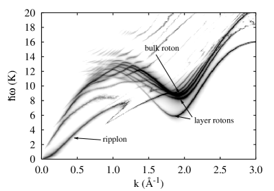
Figure 2: The figure shows the map of the dynamic structure function $S({\bf k},\omega)$ for a ⁴He film for the potential strength $D=32\,$K. The two layer–rotons, the bulk roton, and the ripplon are indicated by arrows.

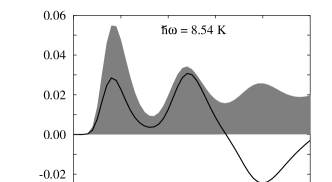
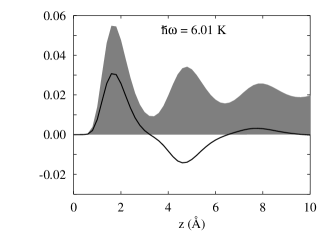
Figure 3: The transition densities of the three lowest excitation are shown for $D=32$ K and $C_{3}=1500$ Kų, normalized to the same maximum value. For comparison, the density profile of the film is shown as a gray–shaded area.

We have carried out two independent calculations of the two–dimensional roton excitation: First, we calculated the roton energy as a function of the density for a rigorously two dimensional liquid. We can assess the accuracy of our predictions with the shadow–wave–function calculation of $S({\bf k},\omega)$ of Ref. Grisenti and Reatto, 1997, who obtained a roton energy of $5.67\pm 0.2\,$K at the equilibrium density of $n=0.0421\,$Å^-2. Second, we have calculated the dynamic structure function $S({\bf k},\omega)$ in the relevant momentum region for the above family of substrate potentials. The results are compiled in Fig. 4 where we also collect several experimental values.

Figure 4: The figure shows the energy of the roton in two dimensions, (long–dashed line) and the energy of the layer roton in a film (solid line) as a function of areal density. The areal densities of the layers were obtained by integrating the density up to the first minimum, the upper horizontal axis shows the corresponding values of the well-depth $D$. Also shown is the energy of a two–dimensional roton obtained with shadow wave functions Grisenti and Reatto (1997) at the density of 0.0421Å^-2. The short–dashed horizontal lines show experimental values of the roton energy on aerogel Fåk et al. (2000); Lauter et al. (2002) (7.39 and 7.14 K), VycorGlyde et al. (2000); Plantevin et al. (2001) (7.23 K), and GeltechPlantevin et al. (2002) (6.71 K), their energies are marked on the right margin.

Although exactly the same method has been used for the computation of the purely two-dimensional system and for the films, the results are quite different. We have obtained for the film calculation an effective layer density by integrating the three-dimensional densities shown in Fig. 1 to the first minimum. This is evidently not very well defined for the weakly bound systems, but it is not legitimate either for the case of strong binding where the first layer is well defined. In fact, the integrated density for the strongest substrate is 0.08 Å^-2, which is well beyond the solidification density of the purely two–dimensional system. Evidently, the zero–point motion in $z$ direction can effectively suppress the phase transition. We make therefore three conclusions: (i) The position of the layer roton minimum is indeed a sensitive measure for the strength of the substrate potential, (ii) purely two–dimensional models are manifestly inadequate for their understanding, and, hence, (iii) purely two–dimensional models are also questionable for interpreting thermodynamic data of adsorbed films.

IV Bulk excitations

With one exception Fåk et al. (2000), the bulk roton energy in porous media have been reported to be practically identical to that in the bulk liquid, Ref. Fåk et al., 2000 reports a slight increase of the roton energy in aerogel at partial filling. A roton energy above the one of the bulk liquid can be explained by assuming that the density of the helium liquid in the medium is below that of the bulk liquid. This can, in turn, be qualitatively explained by the cost in energy to form a surface.

To be quantitative, we have performed calculations of the energetics and structure of ⁴He in a gap between attractive silica walls Apaja and Krotscheck (2003) and obtained the energy of the bulk roton (c.f. Fig. 2) as a function of filling. Fig. 5 shows, as a typical example, the roton energetics in in a gap of 25 Å width. The independent parameter is the areal density $n$, the corresponding three–dimensional density was obtained by averaging the density profile over the full volume. It is seen that the equilibrium density is well below the bulk value. In other words, the roton energy in a confined liquid should correspond to the one of a liquid that would, without confinement, have a negative pressure. The energy increase of the roton minimum found in this model is about 0.5 K, which is consistent with the experiments of Ref. Fåk et al., 2000.

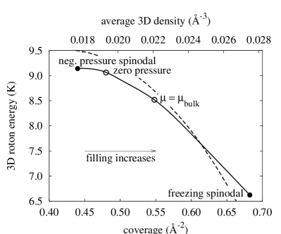
Figure 5: The figure shows the energy of the bulk roton in a gap of 25 Å width as a function of the two–dimensional coverage and the corresponding average density. The points of zero pressure, the low–density and the high–density spinodal points, and the bulk chemical potential are indicated as points. The dashed line shows the roton energy of a purely 3D calculation.

To verify this interpretation of the data, it would be very useful to have comparable measurements for porous media with a more uniform distribution of pore sizes. In particular, comparably small pores should allow to densities that are even below the bulk spinodal density Apaja and Krotscheck (2001), thus facilitating experiments on ⁴He in density areas that were up to now inaccessible.