Recoverable prevalence in growing scale-free networks
and the effective immunization

Abstract

We study the persistent recoverable prevalence and the extinction of computer viruses via e-mails on a growing scale-free network with new users, which structure is estimated form real data. The typical phenomenon is simulated in a realistic model with the probabilistic execution and detection of viruses. Moreover, the conditions of extinction by random and targeted immunizations for hubs are derived through bifurcation analysis for simpler models by using a mean-field approximation without the connectivity correlations. We can qualitatively understand the mechanisms of the spread in linearly growing scale-free networks.

I INTRODUCTION

In spite of the different social, technological, and biological interactions, many complex networks in real-worlds have a common structure based on the universal self-organized mechanism: network growth and preferential attachment of connections Albert01 Barabasi99 . The structure is called scale-free (SF) network, which exhibits a power-law degree distribution $P(k)\sim k^{-\gamma}$, $2<\gamma<3$, for the probability of $k$ connections. The topology deviates from the conventional homogeneous regular lattices and random graphs. Many researchers are attracted to a new paradigm of the heterogeneous SF networks in the active and fruitful area.

The structure of SF networks also gives us a strong impact on the dynamics of epidemic models for computer viruses, HIV, and others. Recently, it has been shown Satorras01a that a susceptible-infected-susceptible (SIS) model on SF networks has no epidemic threshold; infections can be proliferated, whatever small infection rate they have. This result disproves the threshold theory in epidemiology Shigesada97 . The heterogeneous structure is also crucial for spreading the viruses on the analysis of susceptible-infected-recovered (SIR) models May01 Newman02a . In contrast to the absence of epidemic threshold, an immunization strategy has been theoretically presented in SIS models Dezso02 Satorras02 . The targeted immunization applies the extreme disconnections by attacks against hubs with high-degrees on SF networks Albert00a to a prevention against the spread of infections.

In this paper, we investigate the dynamic properties for spreading of computer viruses on the SF networks estimated from real data of e-mail communication Mikami01 . As a new property in both simulation and theoretical analysis, we suggest a growing network with new e-mail users causes the recoverable prevalence from a temporary silence of almost complete extinction. The typical phenomenon in observations Kephart93b White95 is not explained by the above statistical analysises at steady states or mean-values (in the fixed size or $N\rightarrow\infty$). We first consider, in simulations, a realistic growing model with the probabilistic execution and detection of viruses on the SF network. Then, for understanding the mechanisms of recoverable prevalence and extinction, we analyze simpler growing models in deterministic equations. By using a mean-field approximation without the connectivity correlations, we derive bifurcation conditions from the extinction to the recoverable prevalence (or the opposite), which is related to the growth, infection, and immune rates. Moreover, we verify the effectiveness of the targeted immunization by anti-viruses for hubs even in the growing system.

II E-MAIL NETWORK

II.1 The state transition for infection

We consider a network whose vertices and edges represent computers and the communication via e-mails between users. The state at each computer $i=1,\ldots,N$ is changed from the susceptible, hidden, infectious, and to the recovered by the remove of viruses and installation of anti-viruses. We make a realistic model in stochastic state transitions with probabilities of the execution and the detection of viruses. Fig. 1 shows the state transitions, where $\lambda$ and $\delta$ denote the execution rate from the hidden to the infectious state and the detection rate from the special subjects or doubtful attachment files. The probability at least one detection from the $n_{i}$ viruses on the computer is $1-(1-\delta)^{n_{i}}$, and the probability at least one execution is $1-(1-\lambda)^{n_{i}}$. We assume the infected mail is not sent again for the same communication partner (sent it at only one time) to be difficult for the detection. Thus, $n_{i}$ is at most the number of in-degree at each vertex. In the stochastic SHIR model, the final state is the recovered or immune by anti-viruses, if at least one infected mail is received.

Figure 1: S-H-I-R state transition diagram.

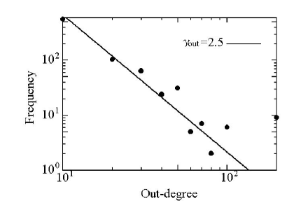
(a)

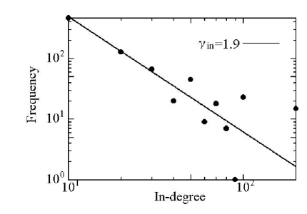
(b)

Figure 2: Power-law degree distributions with the exponents $\gamma_{out}=2.5$ and $\gamma_{in}=1.9$ for (a) sent-mails and (b) receive-mails between users including the internal and the external Mikami01 . The frequency at degree $k$ is counted in the interval between $[k,\;k+10]$, except of the outer of more than 100 degree at $k=200$.

II.2 The scale-free structure

We show the network structure based on real data measured by questionnaires for 2,555 users in a part of World Internet Project 2000 Mikami01 . The distributions of both sent- and receive-mails follow a power-law in Fig. 2, the parameters are estimated as $\gamma_{out}=2.5$, $\gamma_{in}=1.9$, and the average number of mails par day ${\bar{k}}=5\sim 20$. These values are close to the exponents $\gamma_{out}=2.03\pm 0.12$ and $\gamma_{in}=1.49\pm 0.12$ Ebel02 estimated for the server log files of e-mails Data . In addition, the cumulative histograms of less than degree $k$ in Fig. 3 (a) have similar shapes to them in a larger network of e-mail address books Newman02b . The solid lines in Fig. 3 correspond to non-cumulative distributions of the in-degree and out-degree estimated as stretched exponential

(a)

$P_{in}(k)\sim k^{-1.97}\times\exp(-72.26\times k^{-316.23})$, $P_{out}(k)\sim k^{-2.29}\times\exp(-56.98\times k^{-247.39})$,

(b)

$P_{in}(k)\sim k^{-1.82}\times\exp(0.63\times k^{-52.99})$, $P_{out}(k)\sim k^{-2.02}\times\exp(0.6\times k^{-59.23})$,

(c)

$P_{in}(k)\sim k^{-1.75}\times\exp(-0.71\times k^{-53.42})$, $P_{out}(k)\sim k^{-1.39}\times\exp(-1.43\times k^{-137.95})$,

(d)

$P_{in}(k)\sim k^{-2.87}\times\exp(3.54\times k^{-0.048})$, $P_{out}(k)\sim k^{-2.49}\times\exp(3.23\times k^{-0.002})$.

In all of them, the factor of power law as a scale-free network is dominant. Note that the in-degree distribution in Fig. 3 (d) is the most close to the exponential distribution in Newman02b with a strong cut-off, and that both data consists of only the internal networks. However, as in Davidsen02 Newman02b , we must further discuss about the reason why exponential in-degree distribution appears in only the internal networks. This is beyond the scope of this paper. The non-exponential distributions may be caused by the limited size of the sample, or by that the eliminated links from the external nodes have an impact on the generation of hubs in a scale-free network.

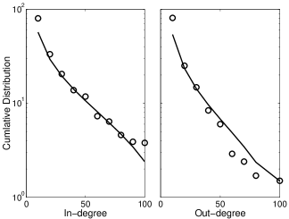
(a)

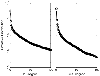
(b)

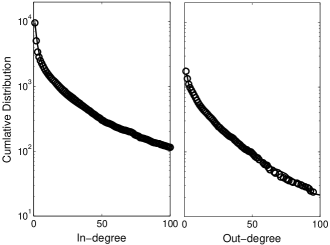
(c)

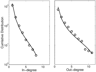
(d)

Figure 3: The cumulative distributions of the in-degree and out-degree for e-mail networks. (a) in the questionnaires Mikami01 , and (b)-(d) in the server log files Data for (b) all of the internal and external nodes as e-mail users, (c) the internal nodes including links from/to the external nodes, and (d) the only internal networks.

II.3 The $(\alpha,\;\beta)$ model

With the estimated parameters, we generate a SF network for the contact relations between e-mail users, by applying the simple $(\alpha,\;\beta)$ model Kumar99 , in which the slopes of power-law $\gamma_{in}\approx\frac{1}{1-\alpha}$ and $\gamma_{out}\approx\frac{1}{1-\beta}$ are controlled by the $\alpha$-$\beta$ coin in Table 1 (in the case of e-mails $\alpha=0.4736$ and $\beta=0.6$). Growing with a new vertex at each step, $k$ edges are added as follows. As the terminal, the coin chooses a new vertex with probability $\alpha$ and an old vertex with probability $1-\alpha$ in proportion to its in-degree. As the origin, the coin chooses a new vertex with probability $\beta$ and an old vertex with probability $1-\beta$ in proportion to its out-degree. According to both the growth and the preferential attachment Albert01 Barabasi99 , the generation processes are repeated until the required size $N$ is obtained as a connected component without self-loops and multi-edges. The $(\alpha,\;\beta)$ model generates both of edges from/to a new vertex and edges between old vertices, the processes are somewhat analogous to ones in the generalized BA model Albert00b Albert01 .

probability	$\alpha$	$1-\alpha$
$\beta$	self-loop at new vertex	origin: new, terminal: old
$1-\beta$	terminal: new, origin: old	both of old vertices

Table 1: Directed edge generation by the $\alpha$-$\beta$ coin.

III SIMULATIONS FOR STOCHASTIC MODEL

We study the typical behavior in the SHIR model on the SF networks. In the following simulations, we set the execution rate $\lambda=0.1$, the detection rate $\delta=0.04$, the average number of edges ${\bar{k}}=6.6$, and initial infection sources of randomly chosen five vertices (the following results are similar to other small values $\lambda=0.2,0.3$ and $\delta=0.05,0.06$). These small values are realistic, because computer viruses are not recognized before the prevalence and it may be executed by some users. We note the parameters are related to the sharpness of increasing/decreasing infections up/down ($\delta$ is more sensitive). It is well known, in a closed system of the SHIR model, the number of infected computers (the hidden and infectious states) is initially increased and saturated, finally converged to zero as the extinction. While the pattern may be different in an open system, indeed, oscillations have been described by a deterministic Kermack-McKendrik model Shigesada97 . However a constant population (equal rates of the birth and the death) or territorial competition has been mainly discussed in the model, the growth of computer network is obviously more rapid, and the communications in mailing are not competitive. Thus, we consider a growing system, in which $50$ vertices and the corresponded new $\bar{k}$ edges are added at every step, from an initial SF network with $N=400$ up to 20350 at 400 steps. Here, one step is corresponding to a day (400 steps $\approx$ a year). These values of $\lambda$, $\delta$, $\bar{k}$, and the growth rate are only examples with something of reality for simulations, since the actual values depends on the observed period are still unknown. As shown in Fig. 4(a)(b), the phenomena of persistent recoverable prevalence are found in the open system, but not in the closed system.

To prevent the wide spread of infections, we investigate how to assign anti-virus softwares onto the SF networks. We verify the effectiveness of the targeted immunization for hubs even in the cases of recoverable prevalence. Fig. 4(c)(d) show the average number of infected computers with recoverable prevalence in 100 trials, where immunized vertices are randomly selected or as hubs according to the out-degree order of the 10 %, 20 %, 30 % of growing size at every 30 steps (corresponded to a month). The number is decreased as larger immune rates for hubs, viruses are nearly extinct (there exists only few viruses) in the 30 % as marked by $\times$ in Fig. 4(c). While it is also decreased as larger immune rates for randomly selected vertices, however they are not extinct even in the 30 % as marked by $\times$ in Fig. 4(d). Fig. 5(a)(b) show the number of recovered states by the hub and random immunization of the 30 % (triangle marks) for the comparison with the normal detections (rectangle marks). The immunized hubs are dominant than the normal detections in Fig. 5(a). However, there is no such difference for the random immunization in Fig. 5(b). In the case of the 10 %, the relation is exchanged; the number of detections is larger than that of both hub and random immunization. It is the intermediate in the case of the 20 %. From these results, we remark the targeted immunization for hubs strongly prevents the spread of infections in spite of the totally fewer recovered states than that in random immunization.

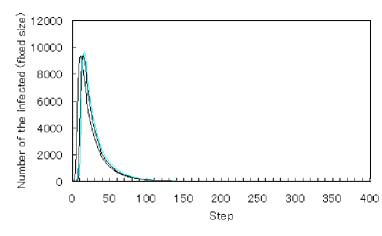
(a)

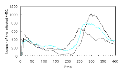
(b)

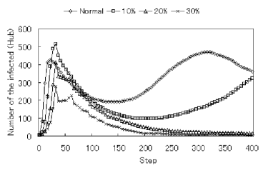
(c)

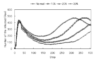
(d)

Figure 4: Typical behavior of the spread on SF networks in (a) a closed system and (b) an open system with simultaneously progress of both spread of viruses and growth of network. The lines show the differences in stochastic state transitions. The effects of immunization are shown as the averages in the open system for (c) hub and (d) random immunization. The open diamond, square, triangle, and cross marks are corresponding to the normal detection by the state transitions, immunization of the 10 %, 20 %, and 30 %, respectively.

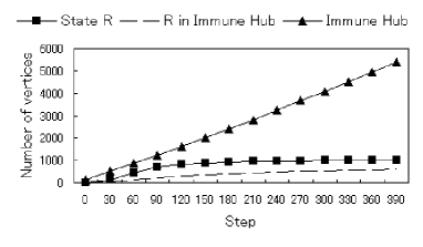
(a)

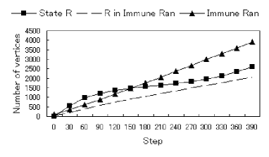
(b)

Figure 5: Number of vertices in the recovered state by (a) hub and (b) random immunization of the 30 %. Each of them is the average value for recoverable prevalence in 100 trials. The dashed lines represent the number of vertices that are already changed to the recovered states before the immunization.

IV ANALYSIS FOR DETERMINISTIC MODEL

Although the stochastic SHIR model is realistic, the analysis is very difficult in the open system. Thus, we analyze simpler deterministic SIR models for the spreading of computer viruses to understand the mechanisms of recoverable prevalence and extinction by the immunization. We consider the time evolutions of $S(t)>0$ and $I(t)>0$ ($t\geq 0$), which are the number of susceptible and infected vertices. We assume that infection sources exist in an initial network, and that both network growth and the spread of viruses are progressed in continuous time as an approximation. In addition, we have no specific rules in growing, but consider a linearly growing network size and the distribution of connections on an undirected connected graph as a consequence.

IV.1 Homogeneous SIR model

As the most simple case, in the homogeneous networks with only the detection of viruses, the time evolutions are given by

$$\frac{dS(t)}{dt} = -b<k>S(t)I(t)+a,$$ (1)

$$\frac{dI(t)}{dt} = -\delta_{0}I(t)+b<k>S(t)I(t),$$ (2)

where $a>0$ and $0<b,\;\delta_{0}<1$ denote the growth, infection, and detection rates, respectively. $<k>\stackrel{{\scriptstyle\rm def}}{{=}}\sum_{k}kP(k)$ is the average number of connections with a probability $P(k)$. The term $S(t)I(t)$ represents the frequency of contact relations. Note that the number of recovered vertices $R(t)$ is a shadow variable defined by $\frac{dR(t)}{dt}=\delta_{0}I(t)$. From the network size $N(t)=S(t)+I(t)+R(t)$, the solution is given by $N(t)=N(0)+at$ as a linear growth. Fig. 6(a) shows the nullclines of

$$\frac{dS}{dt}=0:\;S=\frac{a}{b<k>I},$$

$$\frac{dI}{dt}=0:\;S=S^{*}\stackrel{{\scriptstyle\rm def}}{{=}}\frac{\delta_{0}}{b<k>},\;(I\neq 0)$$

for Eqs. (1)(2). The directions of vector filed are defined by the positive or negative signs of $\frac{dS}{dt}$ and $\frac{dI}{dt}$. There exists a stable equilibrium point $(I^{*},S^{*})$, $I^{*}\stackrel{{\scriptstyle\rm def}}{{=}}\frac{a}{\delta_{0}}$. The states of $S$ and $I$ are converged to the point with a damped oscillation. We can easily check the real parts of eigenvalues for the Jacobian are negative at the point.

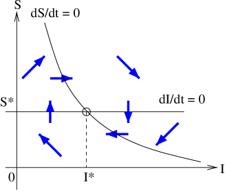
(a)

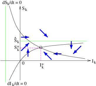
(b)

Figure 6: Nullclines and the vector fields for (a) homogeneous and (b) heterogeneous SIR models. The state in both cases is converged to an equilibrium point with a damped oscillation, which is corresponded to persistent recoverable prevalence around the non-zero level $I^{*}$ or $I^{*}_{k}$.

IV.2 Heterogeneous SIR model

Next, we consider the heterogeneous SF networks at the mean-field level, in which the connectivity correlations are neglected Moreno02 . We know that static and grown networks have different properties for the size of giant component Dorogovtsev01 and the connectivity correlations Callaway01 Krapivsky01 even if the degree distributions are the same. In particular, the correlations may have influence on the spread, however they are not found in all growing network models or real systems. We have experientially observed the correlations are very week in the ($\alpha$, $\beta$) model in the previous simulations as similar to the nearest neighbors average connectivity in the generalized BA model rather than the fitness model or AS in the Internet Satorras01b . At least, non-correlation seems to be not crucial for the absence of epidemic threshold Dezso02 Moreno02 Satorras01a Satorras02 , the existence of correlations is much still less nontrivial in e-mail networks. Although the mean-field approach by neglecting the correlations in macroscopic equations at a large network size is a crude approximation method, it is useful for understanding the mechanisms of the spread in growing networks, as far as it is qualitatively similar to the behavior of viruses in the stochastic model or observed real data. Indeed, the following results are consistent with the analysis for correlated cases Hayashi03 , except of the quantitative differences.

We introduce a linear kernel Krapivsky01 as $N_{k}(t)\sim a_{k}\times t$, $N_{k}(t)=S_{k}(t)+I_{k}(t)+R_{k}(t)$, which are sum of the numbers of susceptible, infected, and recovered vertices with connectivity $k$, and the growth rate $a_{k}\stackrel{{\scriptstyle\rm def}}{{=}}Ak^{-\nu}$, $A>0$, $\nu>2$. Note that the total $N(t)=\sum_{k}N_{k}(t)\sim\left(\sum_{k}a_{k}\right)\times t$ means a linear growth of network size. Since the maximum degree increases as progressing the time and approaches to infinity, it has a nearly constant growth rate $\sum_{k=m}^{\infty}a_{k}\sim\int_{m}^{\infty}Ak^{-\nu}dk=\frac{Am^{1-\nu}}{\nu-1}$ for large $t$. As shown in Krapivsky01 , the introduction of linear kernel is not contradiction with the preferential (linear) attachment Albert01 Barabasi99 .

At the mean-field level in a somewhat large network with only the detection of viruses, the time evolutions of $S_{k}>0$ and $I_{k}>0$ are given by

$$\frac{dS_{k}(t)}{dt} = -bkS_{k}(t)\Theta(t)+a_{k},$$ (3)

$$\frac{dI_{k}(t)}{dt} = -\delta_{0}I_{k}(t)+bkS_{k}(t)\Theta(t),$$ (4)

where the shadow variable $R_{k}(t)$ is implicitly defined by $\frac{dR_{k}(t)}{dt}=\delta_{0}I_{k}(t)$. The factor $\Theta(t)\stackrel{{\scriptstyle\rm def}}{{=}}\sum_{k}c_{k}I_{k}(t)$, $c_{k}\stackrel{{\scriptstyle\rm def}}{{=}}\frac{kP(k)}{<k>}$, represents the expectation that any given edge points to an infected vertex.

We consider a section of $I_{k^{\prime}}=I^{*}_{k^{\prime}}$: const. for all $k^{\prime}\neq k$. Fig. 6(b) shows the nullclines of

$$\frac{dS_{k}}{dt}=0:\;S_{k}=\frac{a_{k}}{kb\Theta}=\frac{a_{k}}{kbc_{k}I_{k}+kb\sum_{k^{\prime}}c_{k^{\prime}}I^{*}_{k^{\prime}}},$$

$$\frac{dI_{k}}{dt}=0:\;S_{k}=\frac{\delta_{0}I_{k}}{kb\Theta}=\frac{\delta_{0}I_{k}}{kbc_{k}I_{k}+kb\sum_{k^{\prime}}c_{k^{\prime}}I^{*}_{k^{\prime}}},$$

and the vector filed for Eqs. (3)(4). There exists a stable equilibrium point $(I^{*}_{k},S^{*}_{k})\stackrel{{\scriptstyle\rm def}}{{=}}(\frac{a_{k}}{\delta_{0}},\frac{a_{k}}{kb\Theta^{*}})$, because of

$$\exists\Theta^{*}=\sum_{k\geq m}c_{k}I^{*}_{k}\sim\frac{A\gamma m^{-\gamma}}{\delta_{0}}\int_{m}^{\infty}k^{-(\nu+\gamma+1)}dk=\frac{A\gamma m^{-\nu}}{\delta_{0}(\nu+\gamma)},$$

by using $c_{k}=\gamma\times m^{\gamma}\times k^{-(\gamma+1)}$ for the generalized BA model Moreno02 with a power-law degree distribution $P(k)=(1+\gamma)m^{1+\gamma}k^{-2-\gamma}$, $<k>=\frac{1+\gamma}{\gamma}m$, (which includes the simple BA model Barabasi99 at $\gamma=1$). On these state spaces in Fig. 6(a)(b), only the case of $a=0$ or $a_{k}=0$ gives the extinction: $I^{*}=0$ or $I^{*}_{k}=0$. It means that we must stop the growing to prevent the infections by the detection. In addition, the homogeneous and heterogeneous systems are regarded as oscillators in Fig. 7(a)(b).

(a)

(b)

Figure 7: Oscillators for (a) homogeneous and (b) heterogeneous SIR models in the open system. They consist of S-I pairs with excitatory: $\rightarrow$ and inhibitory: $\dashv$ connections, and an input bias $a$ or $a_{k}$ of the growth rate. The factor $\Theta$ acts as a global inhibition or excitation.

IV.3 Effect of immunization

We study the effect of random and hub immunization. With the randomly immune rate $0<\delta_{r}<1$, the time evolutions are given by

$$\frac{dS_{k}(t)}{dt} = -bkS_{k}(t)\Theta(t)+a_{k}-\delta_{r}S_{k}(t),$$ (5)

$$\frac{dI_{k}(t)}{dt} = -\delta_{0}I_{k}(t)+bkS_{k}(t)\Theta(t)-\delta_{r}I_{k}(t),$$ (6)

where the shadow variable $R_{k}(t)$ is also defined by $\frac{dR_{k}(t)}{dt}=\delta_{0}I_{k}(t)+\delta_{r}(S_{k}(t)+I_{k}(t))$.

We also consider a section of $I_{k^{\prime}}=I^{*}_{k^{\prime}}$: const. for all $k^{\prime}\neq k$. From the nullclines of Eqs. (5) and (6) with random immunization, there exists a stable equilibrium point $(I^{*}_{k},S^{*}_{k})\stackrel{{\scriptstyle\rm def}}{{=}}(\frac{a_{k}-\delta_{r}S^{*}_{k}}{\delta_{0}+\delta_{r}},\frac{a_{k}}{\delta_{r}+kb\Theta^{*}})$, if the solution

$$\Theta^{*}=\sum_{k}c_{k}I^{*}_{k}=\frac{1}{\delta_{0}+\delta_{r}}\sum_{k}a_{k}c_{k}\left(1-\frac{\delta_{r}}{\delta_{r}+bk\Theta^{*}}\right)\stackrel{{\scriptstyle\rm def}}{{=}}f(\Theta^{*}),$$

is self-consistent at the point. The condition is given by

$$\begin{array}[]{lll}\frac{df}{d\Theta}|_{\Theta=0}&\approx&\frac{Ab}{\delta_{r}(\delta_{0}+\delta_{r})}\int_{m}^{\infty}\gamma m^{\gamma}k^{-(\gamma+\nu)}dk\\ &=&\frac{Ab\gamma m^{-(\nu-1)}}{\delta_{r}(\delta_{0}+\delta_{r})(\gamma+\nu-1)}>1.\end{array}$$

In this case, the state space is the same as shown in Fig. 6(b).

Next, we assume $I^{*}_{k^{\prime}}=0$ for all $k^{\prime}\neq k$ to discuss the extinction. On the section, the nullclines are

$$\frac{dS_{k}}{dt}=0:\;S_{k}=\frac{a_{k}}{\delta_{r}+kb\Theta}=\frac{a_{k}}{\delta_{r}+kbc_{k}I_{k}},$$

$$\frac{dI_{k}}{dt}=0:\;S_{k}=\frac{(\delta_{0}+\delta_{r})I_{k}}{kb\Theta}=\frac{\delta_{0}+\delta_{r}}{kbc_{k}},\;(I_{k}\neq 0)$$

for Eqs. (5)(6). The necessary condition of extinction is given by that the point $(0,\frac{a_{k}}{\delta_{r}})$ on the nullcline $\frac{dS_{k}}{dt}=0$ is below the line $S_{k}=\frac{\delta_{0}+\delta_{r}}{kbc_{k}}$: const. of $\frac{dI_{k}}{dt}=0$. From the condition

$$\frac{a_{k}}{\delta_{r}}<\frac{\delta_{0}+\delta_{r}}{kbc_{k}},$$

we obtain

$$\delta_{r}>-\delta_{0}+\sqrt{\delta_{0}^{2}+4ka_{k}bc_{k}}.$$ (7)

In addition, $0<\delta_{r}<1$ must be satisfied, it is given by $a_{k}<\frac{1+2\delta_{0}}{4b\gamma}$ from $kc_{k}=\gamma m^{\gamma}k^{-\gamma}$, $m\leq k<\infty$, $\gamma>0$, for the generalized BA model Moreno02 . In this case, there exists a stable equilibrium point, otherwise a saddle and a stable equilibrium point as shown in Fig. 8(a)(b). The state space is changed through a saddle-node bifurcation by values of the growth rate $a_{k}$ and the immune rate $\delta_{r}$.

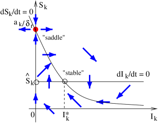
(a)

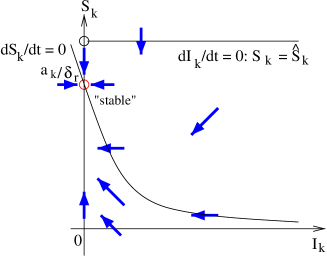
(b)

Figure 8: Saddle-node bifurcation between (a) damped oscillation of recoverable prevalence and (b) convergence to the extinction by the immunization in the heterogeneous SIR model. The state space is changed by the bifurcation parameters $\delta_{r}$ and $a_{k}$ for the value of $\hat{S}_{k}\stackrel{{\scriptstyle\rm def}}{{=}}\frac{\delta_{0}+\delta_{r}}{kbc_{k}}$.

For the hub immunization Dezso02 , $\delta_{r}$ is replaced by $0<\delta_{h}k^{\tau}<1$, $\tau>0$, e.g. $\tau=1$ as proportional immunization to the degree. We may chose the $\frac{1}{k^{\tau}}$ times smaller immune rate $\delta_{h}$ than $\delta_{r}$ for (7). In other words, the necessary condition of extinction in (7) is relaxed to $a_{k}<\frac{m^{\tau}(m^{\tau}+2\delta_{0})}{4b\gamma}$. Thus viruses can be removed in larger growth rate.

The above conditions are almost fitting to the results for the stochastic model in Section III. We can evaluate them using the corresponded parameters: $m=1$, $\nu=2+\gamma=\frac{\gamma_{in}+\gamma_{out}}{2}=2.2$, $b\leftrightarrow\lambda=0.1$, $\delta_{0}\leftrightarrow\delta=0.04$, $\delta_{r}$ or $\delta_{h}=0.1,0.2,0.3$, $\tau=1$, and $A=60$ form $(\sum a_{k})\sim\int Ak^{-\nu}dk=\frac{Am^{1-\nu}}{\nu-1}=50$. By simple calculations, we find that $a_{k}<\frac{1+2\delta_{0}}{4b\gamma}$ is satisfied for $k\geq 2$. The condition (7) is satisfied for only $k\geq 5$ with random immunization of the 30 % and $k\geq 7$ with the 20 %, so the extinction of viruses is difficult by spreading of infection from many vertices with low degree $k\leq 4$, whereas it is satisfied for $k\geq 3$ with hub immunization of both the 20 % and 30 % by the factor of $1/k^{\tau}$. The delicate mismatch at $k=1,2$ may be from the difference of the complicated stochastic behavior as in Fig. 1 and the macroscopic crude approximation.

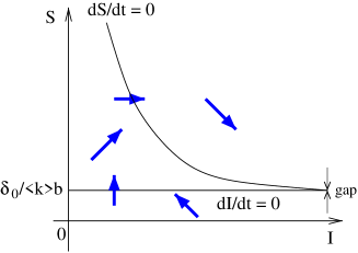
(a)

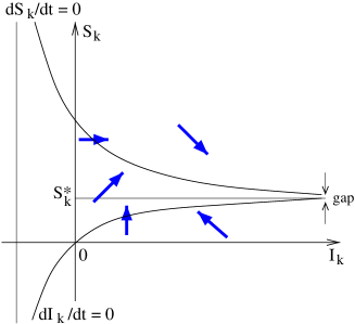
(b)

Figure 9: Non-extinction in (a) homogeneous and (b) heterogeneous SIS models. The number of infected state $I$ or $I_{k}$ finally diverges to infinity.

IV.4 SIS model

Finally, to show the recovered state is necessary, we consider the SIS models in the open system. The time evolutions on homogeneous networks are given by

$$\frac{dS(t)}{dt} = \delta_{0}I(t)-b<k>S(t)I(t)+a,$$ (8)

$$\frac{dI(t)}{dt} = -\delta_{0}I(t)+b<k>S(t)I(t),$$ (9)

where $N(t)=S(t)+I(t)$. The nullclines are

$$\frac{dS}{dt}=0:\;S=\frac{\delta_{0}I+a}{b<k>I}=\frac{\delta_{0}}{b<k>}+\frac{a}{b<k>I},$$

$$\frac{dI}{dt}=0:\;S=\frac{\delta_{0}}{b<k>}:\;{\rm const.},\;(I\neq 0)$$

for Eqs. (8)(9). There exists a gap of $\frac{a}{b<k>I}>0$ even in $I^{*}\rightarrow\infty$. Furthermore, the time evolutions on heterogeneous networks are given by

$$\frac{dS_{k}(t)}{dt} = \delta_{0}I_{k}(t)-bkS_{k}(t)\Theta(t)+a_{k},$$ (10)

$$\frac{dI_{k}(t)}{dt} = -\delta_{0}I_{k}(t)+bkS_{k}(t)\Theta(t).$$ (11)

On a section $I_{k^{\prime}}$: const., the nullclines are

$$\frac{dS_{k}}{dt}=0:\;S_{k}=\frac{\delta_{0}I_{k}+a_{k}}{kb\Theta},$$

$$\frac{dI_{k}}{dt}=0:\;S_{k}=\frac{\delta_{0}I_{k}}{kb\Theta}$$

for Eqs. (10)(11). There also exists a gap between the nullclines. Fig. 9(a)(b) show the nullclines and the vector filed. Thus, the dynamics in the SIS model is quite different from that in the SIR model. We can not realize both of the extinction and the recoverable prevalence of viruses on the SIS model, in any case, even in the open system.

V CONCLUSION

In summary, we have investigate the spread of viruses via e-mails on linearly growing SF network models whose exponents of the power law degree distributions are estimated from a real data of sent- and receive-mails Data or from the generalized BA model Albert01 Moreno02 . The dynamic behavior is the same in both simulations for a realistic stochastic SHIR model and a mean-field approximation without the connectivity correlations for the macroscopic equations of simpler deterministic SIR models. The obtained results suggest that the recoverable prevalence stems from the growth of network, it is bifurcated from the extinction state according to the relations of growth, infection, and immune rates. Moreover, the targeted immunization for hubs is effective even in the growing system. Quantitative fitness with really observed virus data and more detail analysis with the correlations are further studies.

References

- (1) R. Albert, H. Jeong, and A.-L. Barabási. “Error and attack tolerance of complex networks,” nature, vol.406, pp.378-382, 2000.
- (2) R. Albert, and A.-L. Barabási. “Topology of Evolving Networks: Local Events and Universality,” Physical Review Letters, Vol. 85, 5234, 2000.
- (3) R. Albert, and A.-L. Barabási. “Statistical Mechanics of Complex Networks,” arXiv:cond-mat/0106096v1, 2001.
- (4) A.-L. Barabási, R. Albert, and H. Jeong. “Mean-field theory for scale-free random networks,” Physica A, vol.272, pp.173-187, 1999.
- (5) D.S. Callaway et al. “Are randomly grown graphs really random ?,” Physical Review E, Vol. 64, 041902, 2001.
- (6) J. Davidsen, H. Ebel, and S. Bornholdt. “Emergence of a Small World from Local Interations,” Physical Review Letters, Vol. 88, 12870, 2002.
- (7) Z. Dezsö, and A.L. Barabási. “Halting viruses in scale-free networks,” Physical Review E, Vol. 65, 055103, 2002.
- (8) S.N. Dorogovtsev, J.F.F. Mendes, and A.N. Samukhin. “Anomalous percolation properties of growing networks,” Physical Review E, Vol. 64, 066110, 2001.
- (9) H. Ebel, L.-I. Mielsch, and S. Bornholdt. “Scale-free topology of e-mail networks,” Physical Review E, Vol. 66, 035103(R), 2002.
- (10) Y. Hayashi. “Mechanisms of recoverable prevalence and extinction of viruses on linearly growing scale-free networks,” arXiv:cond-mat/0307135, 2003.
- (11) J.O. Kephart, and S.R. White. “Measuring and Modeling Computer Virus Prevalence,” Proc. of the 1993 IEEE Comp. Soc. Symp. on Res. in Security and Privacy, pp. 2-15, 1993.
- (12) P.L. Krapivsky, and S. Render. “Organization of growing networks,” Physical Review E, Vol. 63, 066123, 2001.
- (13) R. Kumar et al. “Extracting large-scale knowledge bases from the web,” Proc. of the 25th VLDB Conf., pp.7-10, 1999.
- (14) R.M. May, and A.L. Lloyd. “Infection dynamics on scale-free networks,” Physical Review E, Vol. 64, 066112, 2001.
- (15) http://sophy.asaka.toyo.ac.jp/users/mikami/info&media/, http://www.commerce.or.jp/result/sp3/index.html, http://www.dentsu.co.jp/marketing/digital_life/
- (16) Y. Moreno, R. Pastor-Satorras, and A. Vespignani. “Epidemic outbreaks in complex heterogeneous networks,” Euro. Phys. J., Vol. 26, 521, 2002.
- (17) M.E.J. Newman. “Spread of epidemic disease on networks,” Physical Review E, Vol. 65, 016128, 2002.
- (18) M.E.J. Newman, S. Forrest, and J. Balthrop. “Email networks and the spread of computer viruses,” Physical Review E, Vol. 66, 035101, 2002.
- (19) R. Pastor-Satorras, and A. Vespignani. “Epidemic dynamics and epidemic states in complex networks,” Physical Review E, Vol. 63, 066117, 2001.
- (20) R. Pastor-Satorras, A. Vázquez, and A. Vespignani. “Dynamical and Correlation Properties of the Internet,” Physical Review Letters, Vol. 87, 258701, 2001.
- (21) R. Pastor-Satorras, and A. Vespignani. “Immunization of complex networks,” Physical Review E, Vol. 65, 036104, 2002.
- (22) N. Shigesada and K. Kawasaki. Biological Invasions: Theory and Practice, Oxford University Press, 1997.
- (23) S.R. White, J.O. Kephart, and D.M. Chess. “Computer Viruses: A Global Perspective,” Proc. of the 5th Virus Bulletin Int. Conf., 1995.
- (24) http://www.theo-physik.uni-kiel.edu/∼ebel/email-net/email-net.html.