Dynamics of shear-transformation zones in amorphous plasticity: non-linear theory at low temperatures

Abstract

We use considerations of energy balance and dissipation to derive a self-consistent version of the shear-transformation-zone (STZ) theory of plastic deformation in amorphous solids. The theory is generalized to include arbitrary spatial orientations of STZs. Continuum equations for elasto-plastic material and their energy balance properties are discussed.

I Introduction

Important progress has been made in a recent series of papers by Falk, Langer and myself on the shear-transformation-zone (STZ) theory of plastic deformation in amorphous solids Langer and Pechenik (2003); Falk et al. (2003). In the first paper in this series we introduced and explored an energetic approach to the STZ theory at temperatures far below glass transition temperature, which helped us to define the limits of the theory’s form. The finite-temperature version of the theory developed in the second paper Falk et al. (2003) allowed us to make predictions that were comparable to to experimental observations of the behavior of bulk metallic glasses (Kato et al.Kato et al. (1998), Lu et al.Lu et al. (2003)). The success and the questions that these studies posed prompt us to look more carefully at the fundamentals of the theory and understand the extent to which the simple approximations that we used were correct, and how to construct the theory without them. This paper is focused on further generalizing and expanding the low-temperature STZ theory of plasticity. In particular, we reexamine the physical significance of two parameters that occurred in the energy balance equations introduced in Ref. Langer and Pechenik (2003); and we show explicitly how to derive the tensorial version of the theory, already used in Ref. Eastgate et al. (2003), that is needed in order to describe situations in which the orientation of the stress changes as a function of position and time. Finally, for completeness, we derive a full set of elasto-plastic continuum equations of motion for this class of models.

The STZ theory of plasticity of amorphous materials at low temperatures was proposed by Falk and Langer in Falk and Langer (1998). It is based on the previous works of Cohen, Turnbull, Spaepen, Argon Turnbull and Cohen (1970); Spaepen (1977); Argon (1979), which argued that non-crystalline solids plasticity is due to atomic rearrangements at localized sites. This picture has also been confirmed by a number of computational studies Srolovitz et al. (1981); Deng et al. (1989). However, unlike the earlier theories, the STZ theory focuses in detail on how rearrangements at the localized sites (shear-transformation-zones) occur, and identifies as important dynamical variables not only the concentration of the STZs, but also their orientations. This new variable allowed immediately to obtain a description of elastic and plastic behavior as an exchange of stability between the two steady states. Such a simple mathematical treatment appears to us to be much more natural than the approach of traditional plasticity theory with its yield criteria.

Moreover, the original STZ theory offered an explanation of a wide class of plasticity phenomena such as work hardening, strain softening, the Bauschinger effect, and others. But, as pointed out in Falk and Langer (1998), it had an inconsistency which implied that the proposed form was not completely correct. The energetic approach introduced in Langer and Pechenik (2003) allowed to correct the inconsistency for a simple case of quasilinear approximation. As shown there, even in such a simple form the STZ theory captured the important features observed in both mechanical tests and calorimetric measurements of glassy polymers at temperatures far below glass transition temperature Hasan and Boyce (1993). A generalization of such an approach (also for the quasilinear approximation) to higher temperatures Falk et al. (2003) has proven to be quantitatively successful in the description of the viscoelastic response of bulk metallic glasses under tensile loadingLu et al. (2003); Kato et al. (1998). However, as argued in Langer and Pechenik (2003); Falk et al. (2003); Falk and Langer (2000), the application of quasilinear theory is limited. Most notably, the quasilinear approximation exaggerates plastic flow at small stresses and low temperatures, and reduces memory effects. As only the non-linear STZ theory can be expected to adequately describe molecular rearrangements, it must be further developed in order to reach precise quantitative agreement with experiment. One of the purposes of this paper is to expand the energetic approach introduced in Langer and Pechenik (2003) to the non-linear STZ theory.

A major challenge in developing the STZ theory was defining the form of the STZ creation and annihilation rates. In the original paper Falk and Langer (1998) these rates were proposed to be proportional to the rate of plastic work $\sigma\dot{\varepsilon}_{pl}$. Since this work can become negative, it was obvious that this form was not acceptable (the inconsistency noted above). An easy (but artificial) remedy was proposed in Eastgate et al. (2003) – to make them proportional to the absolute value $|\sigma\dot{\varepsilon}_{pl}|$. This was sufficient for handling complicated numerical simulations of necking where $\sigma\dot{\varepsilon}_{pl}$ becomes negative during unloading. These simulations also explicitly demonstrated that thinning of the neck could continue even after stretching of the sample had been stopped. This raised a question whether the proposed forms of the STZ theory agreed with fundamental physical principles – the first and second laws of thermodynamics. It appeared that, indeed, they did – the plastic deformation of the neck was driven by the energy stored in the bulk of material, and this process was dissipative.

Beyond that, the involvement of energy concepts in the consideration of the theory opened a different perspective. In this paper we make a conjecture that will be the basis of all of the following discussion – that creation and annihilation rates are proportional to the rate of energy dissipation. This conjecture of proportionality allows us to self-consistently define all components of the theory (Section II). The formalism developed there is a useful tool in limiting the arbitrariness of possible forms of the dynamical equations, transcending the current framework of low-temperature STZ theory. In Section III we demonstrate conclusions of Section II on two important examples.

Another significant limitation of the original STZ theory was that it considered STZs oriented in a single direction only. In earlier studies that had to deal with stress changing its direction Falk (1998); Langer (2000, 2001); Eastgate et al. (2003), the form of the theory for amorphous material, isotropic in its nature, had to be guessed on a phenomenological basis. In Section IV of this paper we return to the microscopic basics and construct a theory that includes STZs oriented in all possible directions. Thereafter, we introduce an approximation that allows us to rewrite the theory in a simpler tensorial form, with order parameters being the first and second moments of the orientational density of the STZs. This tensorial form is comparable to the above mentioned phenomenological theory.

In Section V we combine ideas of the previous sections, applying the energetic approach from Section II to the isotropic model of STZ theory from Section IV.

An understanding of energetic processes in the plastic degrees of freedom allows us to deal more carefully with spatially distributed systems, which we discuss in Section VI. Here we put all of the ingredients together and write dynamical equations for an elasto-plastic material in two dimensions, preserving a clear picture of energy balance.

In Section VII we present some arguments in favor of our conjecture of proportionality between the rate of creation and annihilation of STZs and the rate of energy dissipation. We also discuss some details that have been left out so far, but still may be important to obtain quantitative agreement with experiment.

II Energy concepts in the STZ theory of plasticity

The basic premise of the STZ theory is that the process of plastic deformation in an amorphous material is due to non-affine rearrangements of its particles in certain regions, that are called shear transformation zones. The original STZ theory simplistically considered all STZs as oriented in a single preferred direction. A two-dimensional sample was subjected to pure shear loading with a principal axis of the deviatoric stress tensor coinciding with the preferred direction. Throughout this section we will adhere to the same propositions.

To be specific, we will call the zones elongated along the $y$-axis as “$+$” zones and the zones elongated along the $x$-axis as “$-$” zones. We will denote the density of zones in the “$+$” state by $n_{+}$, and in the “$-$” state by $n_{-}$. For pure shear the deviatoric stress tensor has the form: $s_{xx}=-s$, $s_{yy}=s$, $s_{xy}=0$.

Following Falk and Langer (1998), we can think of the plastic strain rate as the result of transitions between the states of STZs:

$$\dot{\varepsilon}_{pl}=\lambda v\left(R_{-}n_{-}-R_{+}n_{+}\right)\;,$$ (II.1)

where $\dot{\varepsilon}_{pl}$ is the $yy$-component of the plastic strain rate tensor, $R_{+}$ is the rate of transitions from “$+$” to “$-$” states, $R_{-}$ is the rate of transitions from “$-$” to “$+$” states, $\lambda$ is the elementary increment of the shear strain, and $v$ is a volume of the order of the STZ volume. Generally transition rates are functions of stress $s$ or, equivalently, of the dimensionless variable $s/\bar{\mu}$, where $\bar{\mu}$ can be interpreted as a sensitivity modulusFalk and Langer (1998). This modulus has dimension of stress or energy density. Equation (II.1) also implies that all STZs have the same size, and therefore the constants $\lambda$ and $v$ are the same for all zones.

We suppose that STZs can also be annihilated and created, with the annihilation rate $R_{a}$ and creation rate $R_{c}$. The creation rate, unlike transition and annihilation rates, can be understood only as a quantity defined per unit volume. Thus, we have:

$$\dot{n}_{\pm}=R_{\mp}n_{\mp}-R_{\pm}n_{\pm}-R_{a}n_{\pm}+R_{c}\;.$$ (II.2)

We can rewrite Eqs. (II.1), (II.2) in a more convenient form. If we introduce a parameter $\tau_{0}$ that specifies some time scale for transitions, and define rate functions ${\cal S}=\tau_{0}(R_{-}-R_{+})/2$, ${\cal C}=\tau_{0}(R_{-}+R_{+})/2$, ${\cal T}={\cal S}/{\cal C}$, $\Gamma=\tau_{0}R_{a}$, densities $n_{\infty}=2R_{c}/R_{a}$, $n_{tot}=n_{+}+n_{-}$, $n_{\Delta}=n_{+}-n_{-}$, and dimensionless quantity $\epsilon_{0}=\lambda vn_{\infty}$, we get:

$$\tau_{0}\dot{n}_{\Delta} = \frac{2n_{\infty}\tau_{0}}{\epsilon_{0}}\dot{\varepsilon}_{pl}-\Gamma n_{\Delta}\;,$$ (II.3)

$$\tau_{0}\dot{n}_{tot} = \Gamma(n_{\infty}-n_{tot})\;,$$ (II.4)

$$\tau_{0}\dot{\varepsilon}_{pl} = \frac{\epsilon_{0}{\cal C}}{n_{\infty}}\left({\cal T}n_{tot}-n_{\Delta}\right)\;.$$ (II.5)

This system of equations is completely determined if we define the functions $R_{\pm}$, $R_{a}$ and $R_{c}$, which was done in Falk and Langer (1998). In this paper we will postpone choosing specific forms of the transition rates and corresponding functions $\cal C$, $\cal S$, and first focus on the creation and annihilation rates.

From (II.2) we see that an important feature of this theory is that creation and annihilation of STZs are independent of their orientations and occur with equal probability for both orientations. This is not a completely trivial assumption. We disregard the possibility that creation and particularly annihilation can happen in connection with transition processes, and thus be more intense for one orientation of STZs than the other. However, the assumption that the creation and annihilation rates are independent of orientation is simple and plausible. Another observation we can make is that the creation rate is very likely to depend on the structure of material, or in other words, on such characteristics as packing fraction, free volume or structural disorder, as this rate is not only a dynamical, but also a structural property. This is also expressed in the fact that we can define it per volume of material, but not per STZ. On the other hand, the annihilation rate, as well as the transition rates, is less likely to depend on the structure of material. This is expressed in the fact that they can be defined as rates per STZ, and can be thought of as properties of STZs, but not the surrounding material, the influence of which on individual STZs can be described by averaged quantities, such as average stress. In further discussion we will assume that changes in the structure of material can be described by changes in STZ degrees of freedom only. Thus, our only internal dynamical variables are $n_{tot}$ and $n_{\Delta}$, while $n_{\infty}$ is assumed to be a constant.

It was proposed in Falk and Langer (1998) to make the rates of creation and annihilation proportional to the rate of plastic work $2s\dot{\varepsilon}_{pl}$. A peculiarity of this expression mentioned earlier is that these rates, by definition always positive quantities, can become negative. This happens because plastic work does not entirely dissipate.

In general, the rate of plastic work done on a system can be represented in the form

$$2s\dot{\varepsilon}_{pl}=\frac{d\psi}{dt}+{\cal Q}\;,$$ (II.6)

where $\psi$ is the energy that is stored in the plastic degrees of freedom and in principle can be recovered, and $\cal Q$ is the dissipation rate – a non-negative function of stresses and internal variables.

As annihilation and creation rates themselves are non-negative, we propose to make them proportional to the rate of dissipation ${\cal Q}$. We will give some reasons why this proportionality can be true in section VII, but at the moment this proposition should be viewed as a conjecture that provides a physically sensible model and adequately describes mechanical and thermodynamical phenomena in amorphous solids.

Now we are in a position to derive formulas for $\cal Q$, $R_{a}$ and $R_{c}$. We write ${\cal Q}=AR_{a}=A\Gamma/\tau_{0}$, where $A$ is a coefficient determining the proportion in which dissipated energy drives creation and annihilation rates. Generally, this coefficient can be a function of total STZ density $n_{tot}$, but not $n_{\Delta}$, meaning that dissipation produces creations and annihilations of STZs independently of their average orientation already present in the sample. Later we will refine our conjecture and postulate that the annihilation and creation rates are proportional to the rate of energy dissipation not simply per volume, but per STZ. Thus, the coefficient $A$ will be proportional to $n_{tot}$. As the energy $\psi$ depends only on the internal variables $n_{\Delta}$ and $n_{tot}$, we have:

$$\frac{d\psi}{dt}=\frac{\partial\psi}{\partial n_{\Delta}}\dot{n}_{\Delta}+\frac{\partial\psi}{\partial n_{tot}}\dot{n}_{tot}\;.$$ (II.7)

Then, using (II.3), (II.4) and (II.5), we derive from (II.6):

$$\Gamma=\frac{2\tau_{0}\dot{\varepsilon}_{pl}(s-\frac{n_{\infty}}{\epsilon_{0}}\frac{\partial\psi}{\partial n_{\Delta}})}{A-n_{\Delta}\frac{\partial\psi}{\partial n_{\Delta}}+(n_{\infty}-n_{tot})\frac{\partial\psi}{\partial n_{tot}}}\;.$$ (II.8)

In (II.8) we must choose $\psi$ in such a way that $\Gamma$ is always non-negative. If we look at $\Gamma$ as a function of $s$, we conclude that both the numerator and the denominator must always be positive independently. The numerator is guaranteed to be positive if its two factors always become zero simultaneously, that is at $s_{0}=\bar{\mu}{\cal T}^{-1}(n_{\Delta}/n_{tot})$, where ${\cal T}$ is assumed to be monotonic, and ${\cal T}^{-1}$ is the inverse function of ${\cal T}$. This gives:

$$\frac{\partial\psi}{\partial n_{\Delta}}=\frac{\epsilon_{0}\bar{\mu}}{n_{\infty}}{\cal T}^{-1}(n_{\Delta}/n_{tot})\;.$$ (II.9)

From (II.9), it follows that $\psi$ as a function of $n_{\Delta}$ is defined uniquely. If we suppose that the energy $\psi$ must be extensive in $n_{tot}$, we get:

$$\psi=\epsilon_{0}\bar{\mu}\,\frac{n_{tot}}{n_{\infty}}\left(P\left(\frac{n_{\Delta}}{n_{tot}}\right)+\kappa\right)\;,$$ (II.10)

where $P(\xi)=\int_{0}^{\xi}{\cal T}^{-1}(x)\,dx$ and $\kappa$ is a constant. The term proportional to $\kappa$ plays an interesting role here. It determines how much energy is stored in the material due to the presence of the STZs. This energy can be recovered if the sample is annealed and thus the number of STZs is reduced. However, in the low-temperature theory we do not have any way to reduce the density of STZs if it is less than $n_{\infty}$ (see Eq. (II.4)). Therefore, if we are conducting mechanical tests only, this part of the energy appears to be dissipative, although in general it is not.

Now we refine our conjecture and postulate that the annihilation and creation rates are proportional to the dissipation rate per STZ. We can rewrite our equations in a simpler form by defining $\Lambda=n_{tot}/n_{\infty}$, $\Delta=n_{\Delta}/n_{\infty}$, $A=a\epsilon_{0}\bar{\mu}n_{tot}/n_{\infty}$, $\Psi=\psi/\epsilon_{0}\bar{\mu}$, $\tilde{s}=s/\bar{\mu}$. Equations (II.3), (II.4), (II.5), (II.8) and (II.10) then give:

$$\tau_{0}\dot{\Delta} = 2{\cal C}(\tilde{s})({\cal T}(\tilde{s})\Lambda-\Delta)-\Gamma\Delta\;,$$ (II.11)

$$\tau_{0}\dot{\Lambda} = \Gamma(1-\Lambda)\;,$$ (II.12)

$$\tau_{0}\dot{\varepsilon}_{pl} = \epsilon_{0}{\cal C}(\tilde{s})\left(\Lambda{\cal T}(\tilde{s})-\Delta\right)\;,$$ (II.13)

$$\Gamma = \frac{2{\cal C}(\tilde{s})(\Lambda{\cal T}(\tilde{s})-\Delta)(\tilde{s}-{\cal T}^{-1}(\Delta/\Lambda))}{M(\Lambda,\Delta)}\;,$$ (II.14)

$$\Psi = \Lambda(P(\Delta/\Lambda))+\kappa)\;,$$ (II.15)

where the denominator of $\Gamma$ is

$$M(\Lambda,\Delta)=a\Lambda-\frac{\Delta}{\Lambda}{\cal T}^{-1}\left(\frac{\Delta}{\Lambda}\right)+(1-\Lambda)\left(P\left(\frac{\Delta}{\Lambda}\right)+\kappa\right)\;.$$ (II.16)

In earlier papers Langer and Pechenik (2003); Falk et al. (2003), where we used the quasilinear approximation, we chose $a=1$ and $\kappa=1/2$. But these parameters have a physical significance and we will later study how their choice influences the behavior of material.

Let us now look at the locus of the equilibrium points $\dot{\Delta}=0$ in the $\tilde{s}$-$\Delta$ plane (see Fig. 1).

Figure 1: General $\tilde{s}$-$\Delta$ diagram. Here it is plotted for specific parameters of quasilinear model (Sec. III.1), but the diagram’s topology is the same for the general case. The thick solid lines show two steady states – jammed(1) and flowing(2). The arrows show regions where $\Delta$ increases or decreases, which is determined by the sign of $\dot{\Delta}$ from Eq. (II.11). The thick dashed line(3) shows the saturation value of $\Delta$, when $\Lambda=1$. The three thin dashed and dash-dotted lines(4-6) are the $m_{\Lambda}$-lines for fixed $a$ and the three different values of $\kappa$. The thin solid lines(7-10) show quasi-equilibrium branches for those three values of $\kappa$ at some initial value of $\Lambda$.

The importance of these points is due to the fact that they determine the two states of the system – jammed and flowing. The line $\tilde{s}={\cal T}^{-1}(\Delta/\Lambda)$ is the locus of jammed states, here $\dot{\varepsilon}_{pl}=0$. The other solution, $\tilde{s}={\cal T}^{-1}(\Delta/\Lambda)+M(\Lambda,\Delta)/\Delta$, is the locus of flowing states, where $\dot{\varepsilon}_{pl}$ is non-zero. Note the role that $\Lambda$ is playing here. Its equilibrium value is equal to one. Accordingly, the lines plotted for $\Lambda\neq 1$ are not true equilibrium branches. We will call them quasi-equilibrium, as they change when $\Lambda$ relaxes to one.

The jammed and flowing branches can intersect only at the point where $M(\Lambda,\Delta)=0$. The dissipation rate also diverges at this point. In general, the value of the variable $m=\Delta/\Lambda$ at this point is a function of $\Lambda$; we will denote it as $m_{\Lambda}$. Because of the divergence in $\Gamma$, the dynamics of Eq. (II.11) is such that $m$ is always less than $m_{\Lambda}$. Thus, the value of $m_{\Lambda}$ determines the maximum number of STZs that may flip in one direction; we will call it the saturation point.

The function $m_{\Lambda}$ depends on the parameters $a$ and $\kappa$. Let us look at how their choice influences function’s behavior. From Eq. (II.16) we find that when $\Lambda=0$, $m_{\Lambda}=m_{0}$ is the solution of the equation $\kappa=m_{0}{\cal T}^{-1}(m_{0})-P(m_{0})$, and when $\Lambda=1$, $m_{\Lambda}=m_{1}$ is the solution of the equation $a=m_{1}{\cal T}^{-1}(m_{1})$. What happens if $a=a_{\kappa}\equiv m_{0}{\cal T}^{-1}(m_{0})$, so that $m_{1}=m_{0}$? We can check that in this case $M(\Lambda,\Delta)$ vanishes for any $\Lambda$, if $m=m_{0}$, meaning that $m_{\Lambda}\equiv m_{0}$. Thus, we can formulate an important property of Eq. (II.16): for any $\kappa$ there is an $a=a_{\kappa}$, such that $m_{\Lambda}$ is independent of $\Lambda$. The behavior of the function $m_{\Lambda}$ is also simple, if $a$ differs from $a_{\kappa}$. We can prove that if $a>a_{\kappa}$, the function $m_{\Lambda}$ is monotonically increasing, and if $a<a_{\kappa}$, $m_{\Lambda}$ is monotonically decreasing.

To illustrate different choices of parameters $a$ and $\kappa$, in Fig. 1 we show plots of $\Delta=\Lambda m_{\Lambda}$ as functions of $\tilde{s}={\cal T}^{-1}(m_{\Lambda})$, obtained by varying $\Lambda$, for fixed $a$ and three different values of $\kappa$. We will call such curves $m_{\Lambda}$-lines; each of them is the locus of intersection points of the quasi-equilibrium jammed and flowing branches, when $\Lambda$ varies. As the value of $a$ is fixed, steady state branches coincide for different $\kappa$ when $\Lambda=1$. Of the three values of $\kappa$, the intermediate value is such that $a_{\kappa}$ is equal to the given value of $a$.

In an elasto-plastic material the total strain rate is given by

$$\dot{\varepsilon}_{tot}=\dot{\varepsilon}_{pl}+\dot{s}/2\mu\;,$$ (II.17)

where $\mu$ is the shear modulus (see also Eq. (VI.9) and the discussion thereof). Let us consider solutions of the system (II.11-II.13,II.17) at a constant strain rate $\dot{\varepsilon}_{tot}$. If the strain rate is small, the $m_{\Lambda}$-lines coincide with the dynamical trajectories in the regime when $\Lambda$ is evolving from some initial value $\Lambda_{0}$ towards unity. In other words, the dynamical trajectory in the $\tilde{s}$-$\Delta$ plane first moves along the quasi-equilibrium jammed branch calculated for $\Lambda=\Lambda_{0}$ (line 7) until the intersection with the $m_{\Lambda}$-line and then moves along the $m_{\Lambda}$-line (for example, along line 4 for the smallest $\kappa$). For higher strain rates the dynamical trajectories tend to lie to the right of the quasi-equilibrium jammed branch and the corresponding $m_{\Lambda}$-line and evolve from zero to some point on the flowing branch at $\Lambda=1$, determined by the value of $\dot{\varepsilon}_{tot}$. The final value of $\tilde{s}$ can be smaller than intermediate values, thus producing a stress overshoot. As we can see from Fig. 1, a stress overshoot is more likely to happen for large values of $\kappa$. For small values of $\kappa$ the stress increase is usually monotonic.

It is hard to find compelling reasons why in a glassy material the saturation value $m_{\Lambda}$ should be dependent on $\Lambda$. Therefore, we will suppose that for glasses $a=a_{\kappa}$. Indeed, this assumption produces behavior typical for glasses, such as essential strain rate dependence and stress overshoot. Further, we will also study a case when $m_{\Lambda}$ is dependent on $\Lambda$. This case may be relevant for description of polycrystals, clays or soils, if deformation in such systems is due mostly to rearrangement of individual crystals or grains, rather than deformation of grains themselves. The difference from glasses, to which we particularly wish to refer here, is the presence of an additional means of energy dissipation due to friction between constituent particles, which we will model with a larger dissipation coefficient, that is, with $a>a_{\kappa}$.

Now, to make the discussion clear and to put our previous works into the current more general framework, we consider the simple case of what we call the quasilinear version of the STZ theory. Such an analysis was presented in much detail in Langer and Pechenik (2003), albeit only with $a=a_{\kappa}$.

III Examples

III.1 Quasilinear theory

In the quasilinear theory the transition rate functions are supposed to be linear functions of the shear stress $s$. Namely, we assume that ${\cal C}(\tilde{s})=1$, ${\cal S}(\tilde{s})=\tilde{s}$, so that ${\cal T}(\tilde{s})=\tilde{s}$, ${\cal T}^{-1}(\xi)=\xi$, $P(\xi)=\xi^{2}/2$. From (II.15) we get

$$\Psi=\Lambda(m^{2}/2+\kappa)\;,$$ (III.1)

where $m=\Delta/\Lambda$. The expression (II.16) for $M$ becomes

$$M(\Lambda,m)=\Lambda(a-\kappa)+\kappa-(\Lambda+1)m^{2}/2.$$ (III.2)

We find that $m^{2}_{\Lambda}=2(a-\kappa+(2\kappa-a)/(\Lambda+1))$ and $a_{\kappa}=2\kappa$.

In Langer and Pechenik (2003), we chose $a=2\kappa=1$, so that $|m_{\Lambda}|=1$. Then Eq. (II.14) becomes:

$$\Gamma=\frac{4\Lambda(\Lambda\tilde{s}-\Delta)^{2}}{(1+\Lambda)(\Lambda^{2}-\Delta^{2})}\;.$$ (III.3)

Using Eq. (III.3) in the dynamic equations (II.11-II.13) we find that non-flowing steady states occur at $\tilde{s}=\Delta/\Lambda<1$ and flowing steady states at $\tilde{s}=(1+\Lambda)/(2\Delta)-(1-\Lambda)\Delta/(2\Lambda^{2})>1$. The exchange of stability occurs at $\tilde{s}=1$. This value can be naturally associated with the yield stress.

We solve Eqs. (II.11-II.13, II.17) numerically at the constant strain rate and show the results in Fig. 2 (a, b). We plot $\tilde{s}$-$\Delta$ trajectories and stress-strain curves for three initial values of $\Lambda$.

Figure 2: Quasilinear model. $\tilde{s}$-$\Delta$ and stress-strain diagrams for two cases: $m_{\Lambda}$ is constant (Fig. a, b), and $m_{\Lambda}$ is monotonically increasing (Fig. c, d). Lines 1, 2 are the jammed and flowing steady-state branches at $\Lambda=1$, line 3 is the $m_{\Lambda}$-line. Figs. a, c show dynamical trajectories for the stress-strain curves from Figs. b, d respectively.

When the initial number of STZs is small – the sample is annealed – a pronounced stress overshoot is observed. For quenched samples, that is, when the initial value of $\Lambda$ is large, the stress overshoot disappears. As shown in Langer and Pechenik (2003), the constant strain rate simulations of this model are qualitatively similar to the available experimental data Hasan and Boyce (1993).

Now we shall consider other choices of constants $a$ and $\kappa$. One artificial difficulty with the quasilinear approximation is that some choices of these constants lead to $m_{\Lambda}$ larger than unity, thus allowing $m$ to assume non-physical values. To satisfy the condition $|m|\leq 1$, additional conditions must be imposed on the acceptable values of $a$ and $\kappa$. There are two regions for parameters $a$ and $\kappa$, where $|m|\leq 1$ for all $\Lambda$ : (1) when $\kappa\leq 1/2$ and $\kappa\leq a\leq 2\kappa$, here $a\leq a_{\kappa}$, and (2) when $a-\kappa\leq 1/2$ and $2\kappa\leq a$, here $a\geq a_{\kappa}$.

In Fig. 2 (c, d) we plot the results of simulation for $a=1/2$, $\kappa=1/20$, that is, when they are in the second region. The strain rate is small, thus the steady state on the $\tilde{s}$-$\Delta$ diagram almost coincides with the intersection of two steady state branches, and, as discussed in Sec. II, the dynamical trajectory follows along the quasi-equilibrium jammed branch and then along the $m_{\Lambda}$-line. The stress-strain curve exhibits strain hardening as observed in polycrystals, soils or clays Zhu and Yin (2000). Because such a strain-rate curve exists in the limit of an infinitely small strain rate, it can be rate independent for many decades on the logarithmic scale. During strain hardening almost all the energy goes to creating more STZs. As we already noted, we can not get this energy back in mechanical tests, so in this sense, such a regime can be considered to be dissipative.

III.2 Non-linear STZ model

The quasilinear model is very useful as a toy model because of its simplicity. It allows us to proceed much further in analytical and, often, numerical calculations. But it is mainly useful only to gain qualitative insight into the underlying dynamics, not to look for quantitative predictions. The most important drawback of the quasilinear model is its exaggeration of plasticity at small stresses. This drawback can be traced to the form of function ${\cal C}(\tilde{s})$ which is constant in the quasilinear approximation, but in reality is vanishingly small at small stresses. This property is also responsible for suppressing the dynamics of $\Delta$ at small stresses and, thus, for memory effects.

The general derivation of section II suggests that the energetic approach to the fully non-linear model will give qualitatively the same results as those of the quasilinear model, while fixing inaccuracies of the latter. In this subsection we briefly illustrate this point.

In a full STZ model ${\cal C}$ and ${\cal S}$ can be arbitrary non-linear functions of shear stress. The important fact to note is that, unlike what is assumed in the quasilinear approximation, the function $|{\cal T}(\tilde{s})|=|(R_{-}-R_{+})/(R_{+}+R_{-})|$ is always less than unity and asymptotically approaches it when $s\rightarrow\infty$. This causes the function $|{\cal T}^{-1}(m)|$ to diverge when $|m|$ approaches unity. Thus, when the denominator (II.16) vanishes, the value of $|m|=|\Delta/\Lambda|$ is always less than unity. It can not exceed unity at any values of parameters $a$ and $\kappa$, but it also cannot be equal to one. Value of $m$ equal to one corresponds to the complete saturation – the case when all STZs are oriented in one direction. It is puzzling that the non-linear theory does not allow this. But we will see in section V that this is what must happen, if we take into consideration that in amorphous materials the STZs are oriented arbitrarily.

Next, to proceed with numerical calculations we make a particular choice of functions $R_{+}$ and $R_{-}$. We will assume that functions $R_{\pm}$ have the form offered in Falk and Langer (1998), that is $R_{\pm}=\exp\left\{-\beta\exp{(\pm\tilde{s})}\right\}/\tau_{0}$, where $\beta=V^{*}/v_{f}$, $v_{f}$ is the average free volume and $V^{*}$ is of order of the average molecular volume. So we find that

$${\cal C}(\tilde{s}) = \exp{\left(-\beta\cosh\tilde{s}\right)}\cosh{\left(\beta\sinh\tilde{s}\right)}\;,$$

$${\cal S}(\tilde{s}) = \exp{\left(-\beta\cosh\tilde{s}\right)}\sinh{\left(\beta\sinh\tilde{s}\right)}\;,$$

$${\cal T}(\tilde{s}) = \tanh{\left(\beta\sinh\tilde{s}\right)}\;.$$ (III.4)

Figure 3: Nonlinear model. $\tilde{s}$-$\Delta$ and stress-strain diagrams for two cases: $m_{\Lambda}$ is constant (Fig. a, b), and $m_{\Lambda}$ is monotonically increasing (Fig. c, d). Lines 1, 2 are the jammed and flowing steady-state branches at $\Lambda=1$, line 3 is the $m_{\Lambda}$-line. Figs. a, c show dynamical trajectories for the stress-strain curves from Figs. b, d respectively.

Now we can find that the function ${\cal T}^{-1}(m)=\hbox{arcsinh}(\hbox{arctanh}(m)/\beta)$. It diverges logarithmically at $m\rightarrow\pm 1$, but the function $P(m)$ and consequently the plastic energy $\Psi$ given by (II.15) are finite at $|m|=1$.

For the numerical simulations at a constant strain rate loading we used the parameter $\beta=6$. In Fig. 3 (a, b) we have $m_{\Lambda}\equiv 0.992=const$, which is obtained with $a=0.444$, $\kappa=1/3$. The stress rate is large, so that the equilibrium point on the flowing branch (2) is far from the intersection of the jammed (1) and the flowing (2) lines. As in Fig. 2 (a, c), we demonstrate the results for three different values of $\Lambda_{0}$. In Fig. 3 (c, d), we chose $a=0.444$, $\kappa=1/15$, so that the $m_{\Lambda}$-line is monotonically increasing. The strain rate is chosen to be small so the steady state point almost coincides with the intersection of the jammed and flowing branches. Note that analytically we can calculate very little in the fully non-linear model, and even the numerical solution requires not simply solving the system of differential equations, but also numerically calculating the integral $P(m)$ at every step. But the analysis from Sec. II predicts much of the solution’s behavior just from knowing how the function $m_{\Lambda}$ behaves based on the numerical values of $a$ and $\kappa$. We see that the plots in Fig. 3 are very similar to the plots in Fig. 2 for the quasilinear model, since the $\tilde{s}$-$\Delta$ diagrams are topologically the same.

IV Isotropic STZ model of plasticity

In this section we generalize the STZ model of plasticity to the case of arbitrary spatial orientations of STZs and arbitrary orientations of the stress. The first attempt to make such a generalization starting from microscopic basics was made by M. Falk Falk (1998), but was not quite complete.

Here again we will consider a two-dimensional homogeneous sample under a pure shear.

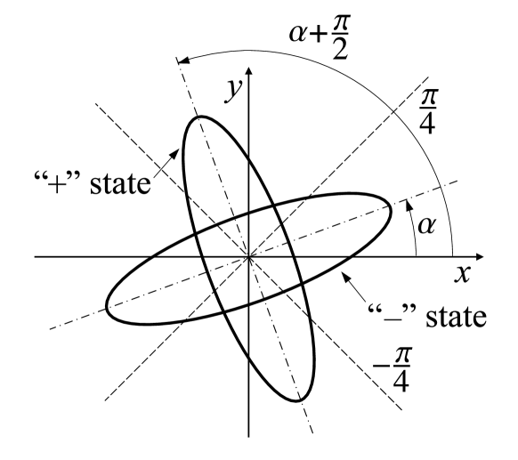
Figure 4: Classification of STZs as being in “+” or “$-$” states.

To be specific, we will classify STZs in relation to the direction of the $x$ and $y$ axes. We will specify that an STZ is in the “$+$” state if the angle between the direction of its elongation and the $y$-axis is smaller than $\pi/4$; when the same is true with respect to the $x$-axis, we will say that the STZ is in the “$-$” state (see Fig. 4). Note, we suppose that the “$+$” and “$-$” orientations of the zone are perpendicular to each other. Deviations from a right angle should be described as fluctuations beyond the mean field theory, and therefore will not be considered here. We write the pure shear in the form $s_{ij}=\bar{s}d^{\phi}_{ij}$, where $\phi$ is the direction of the principal axis of the stress tensor, $\bar{s}=\sqrt{s_{ij}s_{ij}/2}$, and

$$d^{\phi}_{ij}=2\hat{e}^{\phi}_{i}\hat{e}^{\phi}_{j}-\delta_{ij}\;.$$ (IV.1)

In the above equation $\hat{e}^{\phi}_{i}$ is a unit vector in the direction $\phi$, so that $d^{\phi}_{xx}=-d^{\phi}_{yy}=\cos 2\phi$ and $d^{\phi}_{xy}=d^{\phi}_{yx}=\sin 2\phi$. We measure the angle $\phi$ in the counterclockwise direction relative to the $x$-axis. For the purposes of this section we could have chosen the principal axes of the stress tensor to be oriented along the $x$ and $y$ axes, but as we will further want to generalize this discussion for the case of arbitrary temporal evolution of the stress, we suppose that $\phi$ is arbitrary.

Then we suppose that only the diagonal component of the shear stress tensor in the direction of the zone orientation (the projection of the shear stress tensor on that direction) is important for the dynamics of transitions between the states of this zone. Thus, for the dynamics of the STZ population we write:

$$\dot{\chi}_{\alpha}^{+}=R_{-}(s_{\alpha})\chi^{-}_{\alpha}-R_{+}(s_{\alpha})\chi^{+}_{\alpha}-R_{a}\chi_{\alpha}^{+}+R_{c}\;,$$ (IV.2)

$$\dot{\chi}^{-}_{\alpha}=R_{+}(s_{\alpha})\chi_{\alpha}^{+}-R_{-}(s_{\alpha})\chi_{\alpha}^{-}-R_{a}\chi_{\alpha}^{-}+R_{c}\;,$$ (IV.3)

where $\chi_{\alpha}^{\pm}$ is the density of STZs in the “$+$”/“$-$” state oriented at an angle $\alpha$ relative to the $x$ axis, and $s_{\alpha}=\bar{s}d^{\phi-\alpha}_{xx}$ is the projection of the shear stress tensor on the direction $\alpha$. At this moment the density $\chi_{\alpha}^{\pm}$ is defined for angles from $-\pi/4$ to $\pi/4$. Note that all STZs are included in this range due to the circular symmetry.

Now we note that our classification of zones as “$+$” and “$-$” depends on the choice of the direction of $x$ and $y$ axes, which is arbitrary. If one zone is in the “$+$” state in relation to a particular direction, then it is in the “$-$” state in relation to the perpendicular direction, that is, $\chi^{\pm}_{\alpha+\pi/2}=\chi^{\mp}_{\alpha}$. Our dynamical equations should not depend on such arbitrariness; they should give the same results independently of a reference direction. Therefore, Eq. (IV.3) for the angle $\alpha\pm\pi/2$ must be the same as Eq. (IV.2) for the angle $\alpha$, and vice versa. Thus, we conclude that the following relation for transition rates must hold:

$$R_{+}(s_{\alpha})=R_{-}(-s_{\alpha})\;.$$ (IV.4)

We suppose that transitions do not change the volume of material. Thus, we must describe the elementary change in strain by a traceless tensor, which in two dimensions is proportional to $d^{\alpha}_{ij}$. Again, we suppose that the magnitude of this elementary change is always the same, only its orientation can be different. In analogy with Section II we have:

$$\dot{\varepsilon}_{ij}^{pl}=\lambda v\int_{-\pi/4}^{\pi/4}d^{\alpha}_{ij}\left(R_{+}(s_{\alpha})\chi^{+}_{\alpha}-R_{-}(s_{\alpha})\chi^{-}_{\alpha}\right)d\alpha\;.$$ (IV.5)

The region of integration in (IV.5) is chosen to count every STZ only once. However, from the symmetry for the angles $\alpha$ and $\alpha+\pi/2$ we conclude that the same integral is correct with any limits of integration in the form $[-\pi/4+\gamma,\pi/4+\gamma]$.

As in Section II, we can introduce rate functions ${\cal S}=\tau_{0}(R_{-}-R_{+})/2$, ${\cal C}=\tau_{0}(R_{+}+R_{-})/2$, ${\cal T}={\cal S}/{\cal C}$, $\Gamma=\tau_{0}R_{a}$ and also densities $\chi_{\alpha}^{tot}=\chi^{+}_{\alpha}+\chi^{-}_{\alpha}$, $\chi_{\alpha}^{\Delta}=\chi^{+}_{\alpha}-\chi^{-}_{\alpha}$, $\chi_{\infty}\equiv n_{\infty}=2R_{c}/R_{a}$, where, as earlier, tilde means stress rescaled by $\bar{\mu}$, that is $\tilde{s}_{\alpha}=s_{\alpha}/\bar{\mu}$, $\tilde{s}_{ij}=s_{ij}/\bar{\mu}$, $\tilde{\bar{s}}=\bar{s}/\bar{\mu}$. These functions also have symmetry properties: ${\cal S}(\tilde{s}_{\alpha})=-{\cal S}(\tilde{s}_{\alpha+\pi/2})$, ${\cal C}(\tilde{s}_{\alpha})={\cal C}(\tilde{s}_{\alpha+\pi/2})$, ${\cal T}(\tilde{s}_{\alpha})=-{\cal T}(\tilde{s}_{\alpha+\pi/2})$, and $\chi^{tot}_{\alpha}=\chi^{tot}_{\alpha+\pi/2}$, $\chi^{\Delta}_{\alpha}=-\chi^{\Delta}_{\alpha+\pi/2}$. Using these variables we can rewrite Eqs. (IV.2), (IV.3) and (IV.5) as:

$$\tau_{0}\dot{\varepsilon}_{ij}^{pl} = \frac{\epsilon_{0}}{\chi_{\infty}}\int_{-\pi/4}^{\pi/4}d^{\alpha}_{ij}{\cal C}(\tilde{s}_{\alpha})\left({\cal T}(\tilde{s}_{\alpha})\chi^{tot}_{\alpha}-\chi^{\Delta}_{\alpha}\right)d\alpha\;,$$ (IV.6)

$$\tau_{0}\dot{\chi}_{\alpha}^{\Delta} = 2{\cal C}(\tilde{s}_{\alpha})\left({\cal T}(\tilde{s}_{\alpha})\chi^{tot}_{\alpha}-\chi^{\Delta}_{\alpha}\right)-\Gamma\chi_{\alpha}^{\Delta}\;,$$ (IV.7)

$$\tau_{0}\dot{\chi}^{tot}_{\alpha} = \Gamma(\chi_{\infty}-\chi^{tot}_{\alpha})\;.$$ (IV.8)

These equations are analogs of Eqs. (II.3), (II.4), (II.5), but with arbitrary orientations of STZs. Instead of the number of STZs in two different states their variables are the densities of STZs with different orientations. As it is hard to deal with such equations, where $\chi_{\alpha}$ essentially plays the role of a distribution function, we further show that these equations can be simplified under sufficiently relaxed assumptions, and instead of the density $\chi_{\alpha}$ we can introduce its moments – scalar and tensor variables.

Instead of the angular density $\chi^{tot}_{\alpha}$ we can introduce the total density of zones in a sample $n_{tot}=(2/\pi)\int_{-\pi/4}^{\pi/4}\chi^{tot}_{\alpha}d\alpha$, the equation for which is easy to get by integrating Eq. (IV.8). Instead of $\chi^{\Delta}_{\alpha}$ we introduce the tensor $n_{ij}=\int_{-\pi/4}^{\pi/4}d_{ij}^{\alpha}\chi^{\Delta}_{\alpha}d\alpha$. To get dynamical equations for $n_{ij}^{\alpha}$ we multiply Eq. (IV.7) by $d_{ij}^{\alpha}$ and integrate it over $\alpha$:

$$\tau_{0}\dot{n}_{ij}=2\int_{-\pi/4}^{\pi/4}d^{\alpha}_{ij}{\cal C}(\tilde{s}_{\alpha})\left({\cal T}(\tilde{s}_{\alpha})\chi^{tot}_{\alpha}-\chi^{\Delta}_{\alpha}\right)d\alpha-\Gamma n_{ij}\;.$$ (IV.9)

An assumption we will make here is that initially $\chi^{tot}_{\alpha}$ does not depend on $\alpha$. Then according to Eq. (IV.8) $\chi^{tot}_{\alpha}$ is independent of $\alpha$ at all later times. Next, in the integral (IV.9) we will approximate the function ${\cal C}(\tilde{s}_{\alpha})$ by a function $\bar{\cal C}(\tilde{\bar{s}})$ that depends not on the projection of the shear stress tensor on a given direction, but on the principal value of the shear stress $\bar{s}$. The only role that the function $\cal C$ played in the original paper Falk and Langer (1998) was to be responsible for memory effects. It was a vanishingly small function for small stresses, and thus effectively froze the internal variables in an unloaded sample, preserving information about the previous loading. Our approximation keeps such dynamics intact. Now the integral in Eq. (IV.9) can be calculated. Together with Eqs. (IV.6), (IV.8) our system becomes:

$$\tau_{0}\dot{\varepsilon}_{ij}^{pl} = \frac{\epsilon_{0}}{n_{\infty}}\bar{\cal C}(\tilde{\bar{s}})\left(\bar{\cal T}(\tilde{\bar{s}})\frac{s_{ij}}{\bar{s}}n_{tot}-n_{ij}\right)\;,$$ (IV.10)

$$\tau_{0}\dot{n}_{ij} = 2\bar{\cal C}(\tilde{\bar{s}})\left(\bar{\cal T}(\tilde{\bar{s}})\frac{s_{ij}}{\bar{s}}n_{tot}-n_{ij}\right)-\Gamma n_{ij}\;,$$ (IV.11)

$$\tau_{0}\dot{n}_{tot} = \Gamma(n_{\infty}-n_{tot})\;,$$ (IV.12)

where we denoted

$$\bar{\cal T}(\tilde{\bar{s}})=\int_{-\pi/4}^{\pi/4}d\theta{\cal T}(\tilde{\bar{s}}\cos 2\theta)\cos 2\theta\;.$$ (IV.13)

In the derivation of this system we used the previously discussed property that we can change the region of integration to any quadrant. In more detail the integrals in (IV.6) and (IV.9) had been calculated as follows:

$$\int_{-\pi/4}^{\pi/4}d_{ij}^{\alpha}{\cal T}(\tilde{s}_{\alpha})d\alpha = \int_{-\pi/4}^{\pi/4}d_{ij}^{\alpha}{\cal T}(\tilde{\bar{s}}\cos 2(\phi-\alpha))d\alpha=$$

$$= \int_{-\pi/4}^{\pi/4}d_{ij}^{\phi-\theta}{\cal T}(\tilde{\bar{s}}\cos 2\theta)d\theta=d_{ij}^{\phi}\int_{-\pi/4}^{\pi/4}\cos 2\theta\,{\cal T}(\tilde{\bar{s}}\cos 2\theta)d\theta\;,$$

where $d_{ij}^{\phi}$ is equal to $s_{ij}/\bar{s}$.

Equations (IV.10), (IV.11) and (IV.12) give the description of plasticity in the isotropic generalization of the STZ theory.

V The proportionality hypothesis for the isotropic STZ model

We now show how to expand the results of Section II for the isotropic case. Again, as we will want to generalize results of this section for the case of arbitrary temporal evolution of the stress, we suppose that the principal axes of the tensor $s_{ij}$ do not necessarily coincide with the principal axes of the tensor $n_{ij}$. We write the plastic work done on a system as:

$$\dot{\varepsilon}^{pl}_{ij}s_{ij}\equiv\frac{\epsilon_{0}}{\tau_{0}n_{\infty}}s_{ij}\bar{\cal C}(\tilde{\bar{s}})\left(\bar{\cal T}(\tilde{\bar{s}})\frac{s_{ij}}{\bar{s}}n_{tot}-n_{ij}\right)=\frac{d\psi(n_{ij},n_{tot})}{dt}+{\cal Q}\;.$$ (V.1)

We will denote $s_{xx}=-s_{yy}=s$, $s_{xy}=s_{yx}=\tau$, $n_{xx}=-n_{yy}=n_{\Delta}$, $n_{xy}=n_{yx}=n_{\delta}$, and the invariant of the $n_{ij}$ tensor as $\bar{n}=(n_{\Delta}^{2}+n_{\delta}^{2})^{1/2}$. The energy $\psi$ is now a function of three variables, so:

$$\frac{d\psi}{dt}=\frac{\partial\psi}{\partial n_{\Delta}}\frac{dn_{\Delta}}{dt}+\frac{\partial\psi}{\partial n_{\delta}}\frac{dn_{\delta}}{dt}+\frac{\partial\psi}{\partial n_{tot}}\frac{dn_{tot}}{dt}\;.$$ (V.2)

As in Section II, we suppose that ${\cal Q}=a\epsilon_{0}\bar{\mu}n_{tot}\Gamma/\tau_{0}n_{\infty}$. Writing (V.1) in components and then assuming that the energy $\psi$ can depend on $n_{\Delta}$ and $n_{\delta}$ only through $\bar{n}$, we find:

$${\Gamma}=2\bar{\cal C}(\tilde{\bar{s}})\frac{\left(n_{tot}\bar{\cal T}(\tilde{\bar{s}})\frac{s}{\bar{s}}-n_{\Delta}\right)\left(\frac{\epsilon_{0}}{n_{\infty}}\tilde{s}-\frac{\partial\psi}{\partial\bar{n}}\frac{n_{\Delta}}{\bar{n}}\right)+\left(n_{tot}\bar{\cal T}(\tilde{\bar{s}})\frac{\tau}{\bar{s}}-n_{\delta}\right)\left(\frac{\epsilon_{0}}{n_{\infty}}\tilde{\tau}-\frac{\partial\psi}{\partial\bar{n}}\frac{n_{\delta}}{\bar{n}}\right)}{a\epsilon_{0}\bar{\mu}\frac{n_{tot}}{n_{\infty}}-\bar{n}\frac{\partial\psi}{\partial\bar{n}}+(n_{\infty}-n_{tot})\frac{\partial\psi}{\partial n_{tot}}}\;.$$ (V.3)

The rate function $\Gamma=\tau_{0}R_{a}$ must always be positive. In analogy with Section II, considering this expression as a function of stresses allows us to conclude that the numerator and the denominator of $\Gamma$ must always be positive separately. For fixed $n_{\Delta}$, $n_{\delta}$ and $n_{tot}$ and varying $s$, $\tau$ we want the numerator to pass through zero at a single point $(s_{0},\tau_{0})$ and be positive elsewhere. The numerator becomes equal to zero when its first and third brackets are equal to zero. This happens for stresses $s_{0}=n_{\Delta}\bar{s}_{0}/(n_{tot}\bar{\cal T}(\tilde{\bar{s}}_{0}))$ and $\tau_{0}=n_{\delta}\bar{s}_{0}/(n_{tot}\bar{\cal T}(\tilde{\bar{s}}_{0}))$. Now we can express $s_{0}$ and $\tau_{0}$ as functions of the variables $n_{\Delta}$, $n_{\delta}$ and $n_{tot}$ only. Noting that $\bar{s}_{0}=(s_{0}^{2}+\tau_{0}^{2})^{1/2}$, we find that $\bar{s}_{0}=\bar{\mu}\bar{\cal T}^{-1}(\bar{n}/n_{tot})$. Substituting $\bar{s}_{0}$ in the expressions for $s_{0}$ and $\tau_{0}$, we get $s_{0}=\bar{\mu}\bar{\cal T}^{-1}(\bar{n}/n_{tot})n_{\Delta}/\bar{n}$, $\tau_{0}=\bar{\mu}\bar{\cal T}^{-1}(\bar{n}/n_{tot})n_{\delta}/\bar{n}$.

If the second and the fourth brackets also pass through zero at this point, they will always have the same sign as the first and the third brackets correspondingly, ensuring positiveness of the numerator. Thus, from either the second or the fourth bracket we find:

$$\frac{\partial\psi}{\partial\bar{n}}=\frac{\epsilon_{0}\bar{\mu}}{n_{\infty}}\bar{\cal T}^{-1}\left(\frac{\bar{n}}{n_{tot}}\right)\;.$$ (V.4)

Therefore, we find that the energy $\psi$ has the same form as in Section II Eq. (II.10):

$$\psi=\epsilon_{0}\bar{\mu}\frac{n_{tot}}{n_{\infty}}\left(P\left(\frac{\bar{n}}{n_{tot}}\right)+\kappa\right)\;.$$ (V.5)

Now we can write out our final result for the tensorial generalization of the low temperature STZ theory of plasticity in the form analogous to Eqs. (II.11-II.16). If again we denote $\Lambda=n_{tot}/n_{\infty}$, $\Delta_{ij}=n_{ij}/n_{\infty}$, $\bar{\Delta}=\bar{n}/n_{\infty}$, we get:

$$\tau_{0}\dot{\varepsilon}_{ij}^{pl} = \epsilon_{0}\bar{\cal C}(\tilde{\bar{s}})\left(\Lambda\bar{\cal T}(\tilde{\bar{s}})\frac{s_{ij}}{\bar{s}}-\Delta_{ij}\right)\;,$$ (V.6)

$$\tau_{0}\dot{\Delta}_{ij} = 2\bar{\cal C}(\tilde{\bar{s}})\left(\Lambda\bar{\cal T}(\tilde{\bar{s}})\frac{s_{ij}}{\bar{s}}-\Delta_{ij}\right)-\Gamma\Delta_{ij}\;,$$ (V.7)

$$\tau_{0}\dot{\Lambda} = \Gamma(1-\Lambda)\;,$$ (V.8)

$${\Gamma} = \frac{\bar{\cal C}(\tilde{\bar{s}})(\Lambda\bar{\cal T}(\tilde{\bar{s}})s_{ij}/\bar{s}-\Delta_{ij})(\tilde{s}_{ij}-\bar{\cal T}^{-1}(\bar{\Delta}/\Lambda)\Delta_{ij}/\bar{\Delta})}{M(\Lambda,\bar{\Delta})}\;.$$ (V.9)

Expressions $M(\Lambda,\bar{\Delta})$ and $\Psi(\Lambda,\bar{\Delta})=\psi/\epsilon_{0}\bar{\mu}$ are the same as (II.16), (II.15) with $\Delta$ replaced everywhere by $\bar{\Delta}$.

Finally, we can compare our tensorial theory with arbitrary spatial orientations of STZs and arbitrary loading, derived in this section, with the limited STZ theory of Section II for STZs oriented only along two preferred axes and pure shear loading. If we consider pure shear in the generalized STZ theory of this section, we must assume that the principal axes of tensors $s_{ij}$ and $\Delta_{ij}$ are the same. Thus, for pure shear Eqs. (V.6-V.8) become the same as Eqs. (II.11-II.13). Therefore, the results of Section II hold for the STZ theory generalized here. We also note that in the discussion of Section II an important role was played by the saturation point – the value of $m$ for which no further transitions were possible. In the isotropic case, when all STZs are switched in one direction, that is, when $|\chi_{\alpha}^{\Delta}|=\chi^{tot}$, we can find from the expressions for $n_{tot}$ and $n_{ij}$ of Sec. IV that $\bar{n}=n_{tot}$. For other orientational distributions, when $|\chi_{\alpha}^{\Delta}|<\chi^{tot}$ at least in some interval of angles, we have $m=\bar{n}/n_{tot}<1$. However, the projection of the stress tensor on the directions in the narrow strips under angles $\pm\pi/4$ to the principal axes of the stress tensor is small, for any finite value of $\tilde{\bar{s}}$, leading to $|\chi_{\alpha}^{\Delta}|<\chi^{tot}$ at least for those angles. Therefore, we must expect that the saturation point will be reached at $m=\bar{n}/n_{tot}<1$, as has been assumed in Sec. III.2.

VI Continuum equations and energy balance

The plasticity described by the STZ theory can be incorporated into a continuum theory that describes elastic and plastic behavior of viscoelastic solids using a general framework, discussed, for example, in Malvern (1969); Lubliner (1990).

VI.1 The STZ theory of plasticity in a spatially inhomogeneous situation

We start with the generalization of the isotropic STZ model of plasticity for a spatially inhomogeneous situation.

To make the physical picture clear, we will now discuss details omitted for simplicity in the previous sections. Let us consider a small region of material, much smaller than the size of the sample, but much larger than individual atoms and inter-atomic distances. This region contains many STZs of all possible orientations, but from a macroscopic point of view it is infinitesimally small and is identified by its coordinates only. Thus, we are on a mesoscopic scale.

As this region contains many STZs, we consider the average effect of transitions between their states (which are changes in the positions of atoms on the microscopic level) on this region as a small part of the sample. From this point of view the transition between the states of an STZ gives rise to a change of strain at the point where this region is.

Further we will describe the material by what is called the referential description Malvern (1969). Namely, suppose that we are sitting in the material coordinate system and then at some time $t$ we freeze our frame of reference and describe the evolution of the material during an infinitesimally small time interval in this frozen frame of reference. We can see that the discussion of Section IV is correct even for an inhomogeneous situation in the material frame of reference, when the coordinate system not only moves with the particular small region of material, but also rotates with it. In the referential frame of reference we must exclude the effect of translational and rotational motion to make sure that we consider the same region of material under the same angle.

Thus, instead of the time derivative of angle dependent quantities $\chi^{\pm}_{\alpha}$, $\chi^{\Delta}_{\alpha}$, $\chi^{tot}_{\alpha}$, the dot in the expressions (IV.2), (IV.3) and later must denote a complete co-rotational derivative:

$$\dot{\chi}_{\alpha}\equiv\frac{\partial\chi_{\alpha}}{\partial t}+v_{i}\frac{\partial\chi_{\alpha}}{\partial x_{i}}+\omega\frac{\partial\chi_{\alpha}}{\partial\alpha}\;,$$ (VI.1)

where $v_{i}$ and $\omega$ are the translational velocity and the angular speed of our region. When deriving Eq. (IV.9) the integral $\int^{\pi/4}_{-\pi/4}d^{\alpha}_{ij}\dot{\chi}^{\Delta}_{\alpha}d\alpha$ gives the tensorial co-rotational derivative

$$\frac{{\cal D}n_{ij}}{{\cal D}t}\equiv\frac{\partial n_{ij}}{\partial t}+v_{k}\frac{\partial n_{ij}}{\partial x_{k}}+n_{ik}w_{kj}-w_{ik}n_{kj}\;,$$ (VI.2)

where $w_{ij}=1/2(\partial v_{i}/\partial x_{j}-\partial v_{j}/\partial x_{i})$ denotes the spin tensor. This co-rotational derivative must be used in place of $\dot{n}_{ij}$ in (IV.9) and further. Correspondingly, instead of the time derivative $\dot{n}_{tot}$ in the expression (IV.12) we get the total derivative

$$\frac{dn_{tot}}{dt}=\frac{\partial n_{tot}}{\partial t}+v_{i}\frac{\partial n_{tot}}{\partial x_{i}}\;,$$ (VI.3)

as the rotational part integrates out. Finally, in the referential frame of reference the time derivative of the small strain tensor $\dot{\varepsilon}^{pl}_{ij}$ is equal to the rate of deformation tensor $D^{pl}_{ij}$.

Considering the above, the system (IV.10-IV.12) becomes:

$$\tau_{0}D_{ij}^{pl} = \epsilon_{0}f_{\epsilon}(\rho_{0}/\rho)\bar{\cal C}(\tilde{\bar{s}})\left(\bar{\cal T}(\tilde{\bar{s}})\frac{s_{ij}}{\bar{s}}n_{tot}-n_{ij}\right)\;,$$ (VI.4)

$$\tau_{0}\frac{{\cal D}n_{ij}}{{\cal D}t} = 2\bar{\cal C}(\tilde{\bar{s}})\left(\bar{\cal T}(\tilde{\bar{s}})\frac{s_{ij}}{\bar{s}}n_{tot}-n_{ij}\right)-\Gamma n_{ij}\;,$$ (VI.5)

$$\tau_{0}\frac{d{n}_{tot}}{dt} = \Gamma(n_{\infty}-n_{tot})\;.$$ (VI.6)

In (VI.4) we took into account that the elementary strain, which is due to a transition between STZ states, can depend on the local density of material $\rho$ ($\rho_{0}$ denotes some reference density). We will discuss this point later.

VI.2 Continuum theory of elasto-plastic deformation

Here we write out a complete set of equations needed to describe arbitrary elasto-plastic deformation of material. We also make an effort to demonstrate the energy balance properties of our system of equations. This question is certainly not new for a system with constitutive relations in the rate form. However, we consider it important to show how plasticity described by the STZ theory can be incorporated into such a framework.

First, we need to assert that our set of equations contains general equations which are true for any material – the conservation of mass and momentum balance equations:

$$\frac{d\rho}{dt}+\rho\frac{\partial v_{i}}{\partial x_{i}}=0\;,$$ (VI.7)

$$\rho a_{i}=\frac{\partial\sigma_{ij}}{\partial x_{j}}\;,$$ (VI.8)

where $a_{i}$ is the acceleration of material points, which in an inertial coordinate system is equal to $dv_{i}/dt$, and $\sigma_{ij}$ is the true stress.

We describe the material properties by a set of constitutive equations, which also includes equations for internal variables. To describe a viscoelastic solid, we additively decompose the total strain rate tensor $D^{tot}_{ij}=1/2(\partial v_{i}/\partial x_{j}+\partial v_{j}/\partial x_{i})$ as the sum of elastic and plastic parts, which is true under the assumption that elastic strain is small:

$$D^{tot}_{ij}=D^{el}_{ij}+D_{ij}^{pl}\;.$$ (VI.9)

We would like to describe elastic behavior of the material simply by Hooke’s law, but since here we are dealing with large deformations of solids and our equations are in the rate form, we need to take into account at least to some extent the dependence of the elastic properties of the material on its density. As we will see, this is dictated by the conservation of elastic energy. It is convenient to postulate that the equation of state of the material is defined by a function $F_{K}$:

$$p=-Kf_{K}(\rho_{0}/\rho)F_{K}(\rho_{0}/\rho)\;,$$ (VI.10)

such that $f_{K}(x)=F^{\prime}_{K}(x)$, $F_{K}(1)=0$, $f_{K}(1)=1$. In the above equation $p$ is the true pressure and $\rho_{0}$ is the reference density of the material, which is convenient (but not necessary for further discussion) to assume to be the density of the material at zero pressure. The spherical part of the elastic response is fully described by this equation and, in fact, $K$ here is the bulk modulus. Now we can introduce the conjugate stress and strain measures (the strain measure is given implicitly, by defining only the rate of deformation):

$$\tilde{p}=p/f_{K}(\rho_{0}/\rho)\;;\;\;\;\tilde{D}_{ii}=D_{ii}f_{K}(\rho_{0}/\rho)\rho_{0}/\rho\;.$$ (VI.11)

Then, according to (VI.9) and (VI.7), we can write the rate form of Hooke’s law as

$$\tilde{D}^{el}_{ii}=-\frac{1}{K}\frac{d\tilde{p}}{dt}\;,$$ (VI.12)

which coincides with the usual form in the case of small deformations. Similarly, for the deviatoric part of elastic response we have:

$$(\tilde{D}^{el}_{ij})^{dev}=\frac{1}{2\mu}\frac{{\cal D}\tilde{\sigma}_{ij}^{dev}}{{\cal D}t}\;,$$ (VI.13)

where the conjugate stress and strain measures are:

$$\tilde{\sigma}_{ij}^{dev}=\sigma_{ij}^{dev}/f_{\mu}(\rho_{0}/\rho)\;;\;\;\;(\tilde{D}^{el}_{ij})^{dev}=(D^{el}_{ij})^{dev}f_{\mu}(\rho_{0}/\rho)\rho_{0}/\rho\;.$$ (VI.14)

The conservation of mass equation (VI.7), the momentum balance equation (VI.8), the constitutive equations (VI.4), (VI.9), (VI.13), the equation of state (VI.10), and the equations for dynamics of internal variables (VI.5), (VI.6) constitute a full system of equations, which describe elasto-plastic behavior of a material. Those equations possess the property of frame indifference Oldbroyd (1950); Malvern (1969); Lubliner (1990). In particular, we used this system in a simplified form for simulations of necking Eastgate et al. (2003).

The energy balance equation can be derived from the momentum balance equation. This derivation is very well known for the balance of energy in a volume fixed in space, but is less known for the case we are interested in here, when the balance of energy is considered in the volume of material. By multiplying Eq. (VI.8) by $v_{i}$ and integrating over some arbitrary material volume $V$ we get:

$$\int_{(V)}\left(\rho\frac{d}{dt}\frac{v^{2}_{i}}{2}+\frac{\rho}{\rho_{0}}\frac{d}{dt}\frac{\tilde{p}^{2}}{2K}+\frac{\rho}{\rho_{0}}\frac{d}{dt}\frac{(\tilde{\sigma}^{dev}_{ij})^{2}}{4\mu}+D^{pl}_{ij}\sigma_{ij}\right)dV=\int_{(S)}v_{i}\sigma_{ij}dS_{j}\;.$$ (VI.15)

The factor $\rho/\rho_{0}$ in front of the total derivative plays an important role. Without it we would not be able to move differentiation over time in front of the integral. But as $\rho/\rho_{0}$ is the Jacobian of the transformation from the coordinate system $x_{i}(t)$ to the reference state $x_{i}(0)$, we can first change the variable of integration to $x_{i}(0)$, then put the time derivative in front of the integral (instead of a total derivative we will only be left with a derivative over time), and finally we can change variables of integration back to $x_{i}(t)$. This is a purely mathematical procedure. It can be physically interpreted in the following way: instead of integrating over the time varying volume $dV$, we integrate over the conserved mass $\rho dV$. We get:

$$\frac{d}{dt}\int_{(V)}\left(\frac{1}{2}\rho v^{2}_{i}+\frac{\rho}{\rho_{0}}\frac{\tilde{p}^{2}}{2K}+\frac{\rho}{\rho_{0}}\frac{(\tilde{\sigma}^{dev}_{ij})^{2}}{4\mu}+\frac{\rho}{\rho_{0}}\psi\right)dV=$$ (VI.16)

$$\int_{(S)}v_{i}\sigma_{ij}dS_{j}-\int_{(V)}{\frac{\rho}{\rho_{0}}\cal Q}dV\;.$$

Above we also supposed that the plastic work can be expressed as

$$D^{pl}_{ij}\sigma_{ij}=\frac{\rho}{\rho_{0}}\left(\frac{d\psi(n_{ij},n_{tot})}{dt}+{\cal Q}\right).$$ (VI.17)

Equation (VI.16) shows that energy in a particular volume of material consists of kinetic, elastic and plastic parts. It is changed by the work of external forces and it also dissipates due to plastic processes.

An important example relevant to above discussion is the Kirchoff stress tensor $\tilde{\sigma}_{ij}=\sigma_{ij}\rho_{0}/\rho$, which is often used in engineering applicationsMcMeeking and Rice (1975) and standard engineering software ABA (1998). This stress tensor is conjugate to the rate of deformation tensor $D_{ij}$ Hill (1959). We get such a formulation, if we set $F_{K}(x)=\ln x$, $f_{K}=1/x$, $f_{\mu}=1/x$. This formulation assumes the following equation of state: $p=K(\rho/\rho_{0})\ln{\rho/\rho_{0}}$.

Now we return to the assumption (VI.17). For this equation to be valid, the plastic rate of deformation tensor must be dependent on the density of material. This dependency has already been explicitly introduced in (VI.4). At this point it is convenient to generalize our description of plasticity and also take into account the possible dependence of transition rates on the local density of material, which we include in the definition of the stress tensor $s_{ij}$:

$$s_{ij}=\sigma_{ij}^{dev}f_{\epsilon}(\rho_{0}/\rho)\rho_{0}/\rho\;.$$ (VI.18)

Then the density of the rate of plastic work $D_{ij}^{pl}\sigma_{ij}$ can be expressed as a product of $\rho/\rho_{0}$ and a function of $s_{ij}$, $n_{ij}$, $n_{tot}$, but not density. The equation (VI.17) then follows; we used it in the form (V.1) in connection with our hypothesis of proportionality of the annihilation and creation rates to the dissipation rate.

VII Discussion

Now that we have postulated that the rates of STZ creations and annihilations are proportional to the rate of energy dissipation and shown how to derive dynamical equations, we will proceed with discussing physical mechanisms that can underlie this hypothesis, and possible directions to further develop the STZ theory.

The real microscopic picture of plastic deformation is far more complicated than what we describe in our model, where the properties of material are determined by the behavior of STZs only. At present, we can only tell if an STZ exists by observing localized atomic rearrangements – transitions from one STZ state to the other. But in principle an STZ is a spot where transition is potentially possible. However, since we judge about presence of an STZ only after the fact of transition, it is impossible to say whether an STZ was annihilated or created if we did not see its transition; or, even if we saw its transition, it is impossible to say at what point in time the STZ was created or annihilated.

Thus, for example, it is much easier to understand the energetic properties related to a transition that already happened. When atoms in an STZ rearrange, an additional stress field is created around the place of rearrangement. It is in this field that the plastic energy $\psi$ is stored, and this energy is in principle recoverable during a reverse transition.

However, how do we understand the energetic processes related to the elusive events of STZ creations and annihilations? Annihilations are easy to imagine as impossibility of reverse transition after the initial transition or a series of transitions. In this case we can say that the STZ has annihilated and the energy stored in it has dissipated. Hence we can see a direct connection between the dissipated energy and annihilation.

Let us look further. Any transition at low temperatures is a transition from a higher energy state to a lower energy state. This transition and creation of the stress field around the STZ is accompanied by dissipation of energy equal to the difference between the energy levels. This difference, before being absorbed by thermostat, can cause significant local increase of kinetic energy and additional atomic rearrangements which, along with transitions of other STZs, can lead to creations of new STZs and annihilations of existing ones. Thus, the energy dissipation is again related to creations and annihilations.

Another important problem is to consider other essential degrees of freedom describing the structure of material. As we mentioned earlier, $n_{\infty}$ can be especially sensitive to them. In a theory for elevated temperatures, it is the increasing temperature dependence of $n_{\infty}$ that gives calorimetric characteristics of glass transition. An interesting way to introduce a variable describing disorder in the structure of material was offered in Langer (2004), where $n_{\infty}$ was assumed to depend on that new variable instead of directly on the temperature.

In the complex and not yet fully understood picture of the microscopic mechanisms underlying plastic deformation in amorphous solids, the conjecture of proportionality offered in this paper is the simplest of what can be suggested for STZ creation and annihilation rates, and it can be useful beyond the current framework of the low temperature theory.