Lieb-Schultz-Mattis in Higher Dimensions

Abstract

A generalization of the Lieb-Schultz-Mattis theorem to higher dimensional spin systems is shown. The physical motivation for the result is that such spin systems typically either have long-range order, in which case there are gapless modes, or have only short-range correlations, in which case there are topological excitations. The result uses a set of loop operators, analogous to those used in gauge theories, defined in terms of the spin operators of the theory. We also obtain various cluster bounds on expectation values for gapped systems. These bounds are used, under the assumption of a gap, to rule out the first case of long-range order, after which we show the existence of a topological excitation. Compared to the ground state, the topologically excited state has, up to a small error, the same expectation values for all operators acting within any local region, but it has a different momentum.

]

I Introduction

Lieb, Schultz, and Mattis (LSM) proved in 1961 that a one-dimensional periodic chain of length $L$, with half-integer spin per unit cell, has an excitation gap bounded by ${\rm const.}/L$[1]. This behavior contrasts with the possibility of a Haldane gap in the integer spin case[2].

Despite several attempts[3, 4], this theorem has not been extended to higher dimensions. The basic difficulty in obtaining a higher-dimensional version of this theorem was pointed out in two insightful papers by Misguich and coworkers [5]: if spin correlations are short-ranged, the ground state wavefunction should be well described by a short-range resonating valence bond (RVB) state[6]. The short-range RVB basis decomposes into different topological sectors, depending upon the number of dimers crossing a given line through the system. This allows the construction of a low energy excited state very similar to the twisted state of LSM[7]. Instead, if spin correlations are long-ranged, such a state will not be low energy, but there will exist low energy spin wave excitations. In contrast to the one-dimensional case, there now exist two distinct means of obtaining a low energy excitation, significantly complicating the proof of any such theorem.

In the present paper, we show a higher-dimensional version of the LSM theorem. We consider a $d$-dimensional system of spin-$1/2$ spins, with finite-range, $SU(2)$ invariant Hamiltonian $\cal{H}$, and with an odd number of spins per unit cell on the lattice. Define the total number of unit cells in the lattice to be $V$. Let $L$ be the number of unit cells in one particular direction, and let $L$ be even; this direction will be referred to as the length. Therefore, $V$ is even (if $V$ were odd, there would be a trivial spin degeneracy). Let the system be periodic and translationally invariant in the length direction. Let $V/L^{d}$ be bounded by a constant $r$ (this constant $r$ is arbitrary, and imposes some bound on the behavior of the aspect ratio of the system). Define $V/L$ to be the “width” of the system, and let this number be odd. Then, we show that if the ground state is unique, the gap $\Delta E$ to the first excited state satisfies,

$$\Delta E\leq c\log(L)/L,$$ (1)

where the constant $c$ depends on ${\cal H},d$, and where the result holds for all $L$ greater than some minimum $L_{0}$, where $L_{0}$ depends on ${\cal H},d,r$[8].

In this paper, we use the term gap to deal specifically with the difference between the energy of the first excited state and the energy of the ground state. This includes two completely distinct physical cases. In the case of a one-dimensional system, a spin-$1/2$ Heisenberg chain has a continuous spectrum of excitations above the ground state. On the other hand, a Majumdar-Ghosh[9] chain has a doubly degenerate ground state with a gap to the next excited state. Weak perturbations of the Majumdar-Ghosh Hamiltonian can break the exact degeneracy between the two lowest states, leaving a system with a gap from the ground state to the first excited state which is exponentially small in the system size, and then a gap from the first excited state to the next excited state which is non-vanishing even in the limit of large system sizes. We consider both of these cases as systems in which the gap $\Delta E$ is vanishing in the limit of large system size. Although they are one-dimensional systems, these two cases closely match the two possibilities mentioned above for higher-dimensional systems. The first case involves a system with a continuous spectrum as it has algebraically decaying spin correlations. In the second case, the first excited state is very close to the twisted state of LSM.

The physical idea behind the proof of Eq. (1) is closely related to the two possibilities considered above for the absence of a gap. In the event of long-range order, or algebraic long-range order, one expects that there is no gap. Conversely, if there is a gap, one expects that there is no long-range order. This is the first statement we prove: we assume that the system has a gap $\Delta E$ and show, in section III, that connected expectation values decay exponentially in the spacing between them. Then, to prove Eq. (1) we first assume that Eq. (1) is violated, proceeding by contradiction. We assume the existence of such a gap violating Eq. (1) in sections IV, V, and VI. We then use the existence of the gap $\Delta E$ and the exponential decay of correlation functions to show an insensitivity of the system to boundary conditions in section IV. Then, this insensitivity is used to construct a low-energy, twisted state in section V. The construction of this twisted state will to some extent follow the topological attempt[4] at proving the LSM theorem in higher dimensions, with some important differences outlined below. In section VI we will show that the twisted state has a different momentum than the ground state. It is here that the odd width of the system becomes essential. Despite the different momentum compared to the ground state, the twisted state has, up to a small error, the same expectation values for all operators acting within any local region. Thus, we may refer to this state as a topologically excited state. Finally, in an appendix, we briefly consider a version of the result showing exponential decay of correlation functions for systems governed by certain Markov processes, rather than quantum systems.

Since we will constantly deal with operator equations of motion, we introduce a set of “loop operators” as a basic technique. The loop operators, which will be suitably defined products of spin operators, can be naturally interpreted as a product of gauge fields around a loop[10]. However, the use of these operators avoids the uncontrolled approximations associated with the $U(1)$ and $Z_{2}$ gauge theory techniques[11]. The introduction of these operators is not necessary to the main development, but provides a useful notation.

II Loop Algebra

We define operators $i^{\mu\nu}\equiv\frac{1}{2}\delta^{\mu\nu}+\sum_{a}S_{i}^{a}\sigma_{a}^{\mu\nu}$, where $S_{i}^{a}$ are the spin operators at site $i$ and $\sigma_{a}$ are the Pauli matrices, $a=x,y,z$. Thus, $i^{\mu\nu}$ is the two-by-two matrix of spin operators

$$\pmatrix{\frac{1}{2}+S^{z}_{i}&S^{x}_{i}-iS^{y}_{i}\cr S^{x}_{i}+iS^{y}_{i}&\frac{1}{2}-S^{z}_{i}\cr}$$ (2)

We consider operators of the form $i^{\mu\nu}j^{\nu\rho}k^{\rho\sigma}...m^{\alpha\mu},$ which we refer to as loop operators, where a summation over repeated indices is implied. Later we will often suppress the indices $\mu,\nu$, writing $i$ rather than $i^{\mu\nu}$ to save space. Thus, we will write the loop operator mentioned above in the form ${\rm tr}(ijk...m)$, where the trace $tr$ refers to a trace over the Greek indices $\mu,\nu,...$. Below we also use a trace $Tr$; this trace $Tr$ refers to a trace of quantum operators, summing over all states in the Hilbert space of the system. Using the rule $i^{\mu\nu}i^{\rho\sigma}=\delta^{\nu\rho}i^{\mu\sigma}$, it is always possible to reduce a given product of traces to a new product such that each site appears only once. Then, an operator ${\rm tr}(ijk...m)$ permutes the spins around the sites $i,j...$

Given an operator $O(t)$, the operator obeys the equation of motion $\partial_{t}O(t)=-i[O,{\cal H}]$. Consider, for example a term ${\rm tr}(ij)$ in ${\cal H}$. We have $[i,{\rm tr}(ij)]=ij-ji$. As an illustration, let us give the full Greek indices on this commutator: we have $[i^{\mu\nu},(i^{\alpha\beta}j^{\beta\alpha})]=i^{\mu\alpha}j^{\alpha\nu}-j^{\mu\alpha}i^{\alpha\nu}$, where summation over repeated indices $\alpha,\beta$ is assumed.

Introduce coordinates $(x,y)$ to specify sites $i$, where $x$ labels the unit cells along the direction of length and is defined up to integer multiples of $L$. The coordinate $y$ labels the unit cells along the other lattice directions, as well as labeling the particular spin within the unit cell. Given two sites $i$ and $j$ on the lattice, we define the distance between them, written $|i-j|$, as the minimum number of moves by lattice vectors needed to move from the unit cell containing $i$ to that containing $j$. On a square lattice, for example, this is the Manhattan distance. Then, let $R$ denote the range of ${\cal H}$, the furthest distance between two sites in any term in ${\cal H}$. If all distances in a product of loops are less than $L/2$, we can define a winding number of the given product around the lattice in the length direction. If all distances in the product remain less than $L/2-R$, then the dynamics ${\partial_{t}O}=-i[O,{\cal H}]$ does not connect sectors with different winding numbers. We will make use of the coordinates later by sometimes writing loop operators ${\rm tr}(ij...)$ in the form ${\rm tr}((x_{1},y_{1})(x_{2},y_{2})...)$, where $i$ has coordinates $(x_{1},y_{1})$, $j$ has coordinates $(x_{2},y_{2})$, and so on.

III Locality

We consider ground state expectation values of operators $O_{1},O_{2}...$, written $\langle O_{1}(t_{1})O_{2}(t_{2})...\rangle$. The expectation values are not time ordered: the ordering of operators is as written. For a system with a unique ground state and an energy gap $\Delta E$, on physical grounds one expects that connected correlation functions, defined as $\langle A(0)B(0)\rangle_{c}\equiv\langle A(0)B(0)\rangle-\langle A(0)\rangle\langle B(0)\rangle$, decay exponentially in distance (without loss of generality, we will assume $\langle A\rangle=\langle B\rangle=0$ through the rest of this section). The proof of this locality bound will be done in this section. We will do this in two steps: first, we consider commutators of the form $[A(t),B(0)]$, where $A(0)$ and $B(0)$ are separated in space. We bound the operator norm[13] of the commutator for sufficiently small $t$, and thus bound its expectation value, in Eq. (8) below. The proof in this subsection will just be sketched; a more rigorous derivation is due to Lieb and Robinson[14]. This result provides a bound on the velocity of the system, as will be seen below. Then, in the next subsection, from this bound on the expectation value of the commutator and the existence of a gap, we use a spectral representation of the commutator to bound the connected correlation functions, thus obtaining the desired locality bound on the expectation value, Eq. (22). Finally, we close the section by giving a similar locality bound for operators separated in time.

A Finite Velocity

We define the distance between two operators $O_{1},O_{2}$ to be $l$ if the minimum distance between any pair of sites, $i,j$, where $S_{i}$ appears in $O_{1}$ and $S_{j}$ appears in $O_{2}$, is $l$. $A(0),B(0)$ are sums of products of spin or loop operators, which we suppose to be distance $l$ apart.

We start with some notation. The Hamiltonian, ${\cal H}$, can be written as a sum of terms ${\cal H}=\sum_{i}{\cal H}_{i}$, such that each ${\cal H}_{i}$ only contains spins operators on sites $j$ with $|i-j|\leq R$. Let $N_{A}$ denote the number of sites appearing in $A(0)$, and $N_{B}$ denote the number of sites appearing in $B(0)$. Let $J$ denote the maximum, over sites $i$, of $||{\cal H}_{i}||$.

We now bound the operator norm of the commutator $[A(t),B(0)]$ for short times. On short time scales, one expects that $A(t),B(0)$ are still separated in space, up to small correction terms, as we now show. Consider first $||[A(t),{\cal H}_{i}]||$, and study the change in this quantity as a function of time:

$$|\frac{||[A(t)-i{\rm d}t[A(t),{\cal H}],{\cal H}_{i}]||-||[A(t),{\cal H}_{i}]||}{{\rm d}t}|$$ (3)

$$=|\frac{||[A(t),{\cal H}_{i}+i{\rm d}t[{\cal H}_{i},{\cal H}]]||-||[A(t),{\cal H}_{i}]||}{{\rm d}t}|$$ (4)

$$\leq\sum\limits_{|i-j|\leq 2R}|\frac{||[A(t),{\cal H}_{i}+i{\rm d}t[{\cal H}_{i},{\cal H}_{j}]]||-||[A(t),{\cal H}_{i}]||}{{\rm d}t}|$$ (5)

$$=\sum\limits_{|i-j|\leq 2R}|\frac{||[A(t)-i{\rm d}t[A(t),{\cal H}_{j}],{\cal H}_{i}]||-||[A(t),{\cal H}_{i}]||}{{\rm d}t}|$$ (6)

$$\leq 2J\sum\limits_{|i-j|\leq 2R}||[A(t),{\cal H}_{j}]||.$$ (7)

Here, we work to linear order in ${\rm d}t$. While the operator $[A(t),{\cal H}_{j}]$ is differentiable, its operator norm need not be. Thus, all equations here are correct when we take the lim sup as ${\rm d}t\rightarrow 0$.

The first equality in Eq. (3) is obtained by moving the time derivative from $A(t)$ to ${\cal H}_{i}$ as follows: for any operator $P$, to linear order in ${\rm d}t$ we have $||P||=||P+i{\rm d}t[P,{\cal H}]||$. Set $P=[A(t)-i{\rm d}t[A(t),{\cal H}],{\cal H}_{i}]$. Then, to linear order in ${\rm d}t$, $||P||=||P+i{\rm d}t[P,{\cal H}]||=||[A(t)-i{\rm d}t[A(t),{\cal H}],{\cal H}_{i}]+i{\rm d}t[[A(t),{\cal H}_{i}],{\cal H}]||=||[A(t),{\cal H}_{i}+i{\rm d}t[{\cal H}_{i},{\cal H}]]||$.

The inequality is obtained because $[{\cal H}_{i},{\cal H}_{j}]=0$ for $|i-j|>2R$. The next equality is obtained by moving the time derivative back to $A(t)$, using now the equality $||P||=||P-i{\rm d}t[P,{\cal H}_{j}]||$. The final inequality results from the bound $||{\cal H}_{i}||\leq J$.

Now, let $S$ denote the maximum number of sites $j$ within distance $R$ of any site $i$. Eq. (3) gives a set of differential equations which bound the operator norm of various commutators; we have also the initial conditions that $||[A(0),{\cal H}_{j}]||$ vanishes for sites $j$ which are further than distance $R$ from any site in $A(0)$, while $||[A(0),{\cal H}_{j}]||\leq 2J||A||$ for all other sites. The number of sites within distance $R$ of $A(0)$ is bounded by $N_{A}S$.

To bound $||[A(t),{\cal H}_{j}]||$, let us then consider the following set of differential equations: for $t>0$, we take $\partial_{t}G_{i}=2J\sum_{|i-j|\leq 2R}G_{j}$ and for $t<0$ we take $\partial_{t}G_{i}=-2J\sum_{|i-j|\leq 2R}G_{j}$, with initial conditions $G_{j}=0$ for sites $j$ which are further than distance $R$ from any site in $A(0)$, and $G_{j}=2J||A||$ for all other sites. Then, comparing these equations to Eq. (3), we see that $||[A(t),{\cal H}_{i}]||\leq G_{i}(t)$. This set of linear equations for $G_{i}$ can be solved for any given lattice. However, we are simply interested in an upper bound on $G_{i}$. Let us define $G^{k}$ to be the maximum of $G_{i}$ over all sites $i$ which are at a distance greater than $(2k-1)R$ from all sites in $A(0)$. Then, we have $\partial_{t}G^{k}\leq 2JSG^{k-1}$ for $k>0$, and $\partial_{t}G^{k}\leq 2JSG^{k}$ for $k=0$, with initial conditions $G^{0}=2J||A||$ and $G^{k}=0$ for $k\geq 1$. Thus, $G^{0}(t)\leq 2J||A||e^{2JSt}$, $G^{1}(t)\leq\int_{0}^{t}{\rm d}t^{\prime}2JSG^{0}(t^{\prime})\leq\int_{0}^{t}{\rm d}t^{\prime}(2JS)(2J||A||)e^{2JSt}=2J||A||(2JSt)e^{2JSt}$, and $G^{k}(t)\leq 2J||A||(2JSt)^{k}e^{2JSt}/k!$. The last set of inequalities follows inductively: $G^{k}(t)\leq\int_{0}^{t}{\rm d}t^{\prime}(2JS)G^{k-1}(t)\leq\int_{0}^{t}{\rm d}t^{\prime}(2JS)(2J||A||)(2JSt^{\prime})^{k-1}/(k-1)!e^{2JSt}=2J||A||(2JSt)^{k}e^{2JSt}/k!$. From these inequalities, we find, for a site $j$ which is at a distance greater than $(2k-1)R$ from $A(0)$, that $||[A(t),{\cal H}_{j}]||\leq 2J||A|||2JSt|^{k}e^{2JS|t|}/k!$.

Finally, consider $\partial_{t}||[A(t),B(0)]||$. Using a similar sequence of inequalities to Eq. (3), we find that $\partial_{t}||[A(t),B(0)]||\leq 2||B||\sum_{j}||[A(t),{\cal H}_{j}]||$, where the sum over $j$ extends over sites $j$ which are within distance $R$ of some sites in $B(0)$. There are at most $N_{B}S$ such sites, and each of them has $||[A(t),{\cal H}_{j}]||\leq G^{k-1}(t)$, where $k=l/2R$. Here, we take $k$ to be the ceiling of $l/2R$, the smallest integer greater than or equal to $l/2R$; we obtain this value of $k$ since each such site is at least a distance $l-R$ from all sites in $A(0)$, and so we need $l-R>[2(k-1)-1]R$. Then, $||[A(t),B(0)]||\leq 2N_{B}||A||||B|||2JSt|^{l/2R}e^{2JS|t|}/(l/2R)!$.

Define $f(t)\equiv\langle[A(t),B(0)]\rangle$. Since $f(t)\leq||[A(t),B(0)]||$,

$$f(t)\leq\frac{2N_{B}||A||||B|||2JSt|^{l/2R}e^{2JS|t|}}{(l/2R)!}$$ (8)

$$\equiv N_{B}||A||||B||g(t,l).$$ (9)

For $t=c_{1}l$, the large $l$ behavior of $g(t,l)\sim\exp[(l/R)(2JSc_{1}R+1/2+(1/2){\log}(4JSc_{1}R))]$. If we choose a sufficiently small $c_{1}$, then $g(c_{1}l,l)$ decays exponentially in $l$ for large $l$. Numerically, we find that the zero of $2JSc_{1}R+1/2+(1/2){\log}(4JSc_{1}R))]$, is at $c_{1}\approx 0.139232/(2JSR)$. Any $c_{1}$ smaller than this value (for example, $c_{1}=0.1/(2JSR)$ will work) will cause $g(c_{1}l,l)$ to be exponentially decaying for large $l$. The velocity at which correlations spread in the system is of order $c_{1}^{-1}$.

B Spectral Decomposition

Now, we use a spectral decomposition of $f(t)$ to relate $f(t)$ to the desired correlation function, $\langle A(0)B(0)\rangle$. Without loss of generality, let us set the ground state energy, $E_{0}$, to $0$. The spectral decomposition of $f(t)$ gives

$$f(t)=\sum_{i}(e^{-iE_{i}t}A_{0i}B_{i0}-e^{iE_{i}t}B_{0i}A_{i0}),$$ (10)

where $A_{i0}$ is the matrix element of operator $A$ between the ground state $0$ and the eigenstate $i$, with energy $E_{i}\geq\Delta E$ above the ground state energy, and similarly for the other $A_{0i},B_{i0},B_{0i}$. There are no terms in Eq. (10) involving $A_{00},B_{00}$ since we have assumed $\langle A\rangle=\langle B\rangle=0$.

Let us define a function $f^{+}(t)=\sum_{i}e^{-E_{i}t}A_{0i}B_{i0}$, which thus contains only the negative frequency (positive energy) terms in $f(t)$. The significance of $f^{+}(t)$ is that $f^{+}(t)=\langle A(t)B(0)\rangle$, so that the positive energy part of $f(t)$ contains the desired correlation function in it. In this subsection, we combine the bound (8) on $f(t)$ with the existence of a gap to bound $f^{+}(0)$.

Define $\tilde{f}(t)=f(t)e^{-t^{2}\Delta E^{2}/(2q)}$, with $q$ to be chosen later. We have two bounds on $\tilde{f}(t)$. First, we have the bound (8) on $f(t)$ which gives us the bound $\tilde{f}(t)\leq N_{B}||A||||B||g(t,l)$. We also have have

$$\tilde{f}(t)\leq 2||A||||B||e^{-t^{2}\Delta E^{2}/(2q)}.$$ (11)

We will use the first of these bounds for times $|t|<c_{1}l$, and the second for long times $|t|>c_{1}l$. Finally, we define ${\tilde{f}}^{+}(t)$ to contain only the negative frequency terms in $\tilde{f}(t)$.

Now, the desired expectation value $\langle A(0)B(0)\rangle=f^{+}(0)$. To bound $f^{+}(0)$, we first bound ${\tilde{f}}^{+}(0)$, and then bound ${\tilde{f}(0)}^{+}-f^{+}(0)$. To bound ${\tilde{f}}^{+}(0)$, we use the bounds on $\tilde{f}$ and an integral representation of the positive energy part[15, 16]:

$$|{\tilde{f}}^{+}(0)|=\frac{1}{2\pi}|\int_{-\infty}^{\infty}{\rm d}t\,\tilde{f}(t)/(-it+\epsilon)|$$ (12)

$$=\frac{1}{2\pi}\Bigl{(}|\int_{|t|<c_{1}l}\tilde{f}(t)/(-it+\epsilon)|+|\int_{|t|>c_{1}l}\tilde{f}(t)/(-it+\epsilon)|\Bigr{)}$$ (13)

$$\leq\frac{1}{2\pi}||A||||B||\Bigl{(}2N_{B}g(c_{1}l,l)+2\frac{\sqrt{2\pi q}}{\Delta Ec_{1}l}e^{-c_{1}^{2}l^{2}\Delta E^{2}/(2q)}\Bigr{)}.$$ (14)

In Eq. (12), to bound the integral over $|t|<c_{1}l$, we used $|\tilde{f}(t)|\leq|f(t)|\leq N_{B}||A||||B||g(t,l)\leq N_{B}||A||||B||[|t|/(c_{1}l)]g(c_{1}l,l)$. To derive this inequality we have assumed that $l>0$ so that taking the ceiling of $l/2R$ above gives a $k\geq 1$. Then,

$$|\int_{|t|<c_{1}l}{\rm d}t\tilde{f}(t)/(-it+\epsilon)|\leq$$ (15)

$$N_{B}||A||||B||\int_{|t|<c_{1}l}{\rm d}tg(c_{1}l,l)/(c_{1}l)=$$ (16)

$$2N_{B}||A||||B||g(c_{1}l,l).$$ (17)

To bound the integral over $|t|>c_{1}l$ in Eq. (12) we have used Eq. (11) to show $|\int_{|t|>c_{1}l}\tilde{f}(t)/(-it+\epsilon)|\leq 2||A||||B||\int_{-\infty}^{\infty}{\rm d}t\exp[-t^{2}\Delta E^{2}/(2q)]/(c_{1}l)\leq 2||A||||B||\frac{\sqrt{2\pi q}}{\Delta Ec_{1}l}\exp[-c_{1}^{2}l^{2}\Delta E^{2}/(2q)]$.

To bound $|{\tilde{f}(0)}^{+}-f(0)^{+}|$, we start with the definition of $\tilde{f}$. Expressed as a convolution in Fourier space[17] this is:

$$\tilde{f}(\omega^{\prime})=(\sqrt{2\pi q}/\Delta E)\int d{\omega}f(\omega)e^{-q(\omega-\omega^{\prime})^{2}/(2\Delta E^{2})}.$$ (18)

Now is where the existence of an energy gap becomes essential. For motivation, let us first pictorially (see Fig. 1) describe how the gap enables us to bound $|{\tilde{f}^{+}(0)}-f^{+}(0)|$ and then present it more mathematically. By definition $\tilde{f}(0)=f(0)$; this follows in Fourier space from $\int_{-\infty}^{\infty}{\rm d}\omega f(\omega)=\int_{-\infty}^{\infty}{\rm d}\omega\tilde{f}(\omega)$. The convolution (18) means that a given Fourier component in $f$ which is, for example, negative frequency, will produce both positive and negative frequency Fourier components in $\tilde{f}$. So, consider a $\delta$-function spike in $f(\omega)$, produced by an intermediate state $i$ with energy $E_{i}=-\omega>0$. This produces a Gaussian in $\tilde{f}(\omega)$, as shown. The integral over all $\omega$ of the Gaussian is the same as the integral of the $\delta$-function; however, the shaded portion of the curve has $\omega>0$. Since $\tilde{f}^{+}(0)=(2\pi)^{-1}\int_{-\infty}^{0}{\rm d}\omega\tilde{f}(\omega)$ and $f^{+}(0)=(2\pi)^{-1}\int_{-\infty}^{0}{\rm d}\omega f(\omega)$, we find a difference between $\tilde{f}^{+}(0)$ and $f^{+}(0)$ equal to the integral of the shaded portion of the curve. At $\omega=0$ the height of the Gaussian is reduced by a factor $e^{-q\omega^{2}/(2\Delta E^{2})}$. However, since $E_{i}\geq\Delta E$, this factor is bounded by $e^{-q/2}$.

Now, let us do the calculation more directly: $\tilde{f}^{+}(0)=(2\pi)^{-1}\int_{-\infty}^{\infty}{\rm d}\omega f(\omega)\int_{-\infty}^{0}{\rm d}\omega^{\prime}(\sqrt{2\pi q}/\Delta E)\exp[-q(\omega-\omega^{\prime})^{2}/(2\Delta E^{2})]$, while $f^{+}(0)=(2\pi)^{-1}\int_{-\infty}^{0}{\rm d}\omega f(\omega)$. Then

$$\tilde{f}^{+}(0)-f^{+}(0)=(2\pi)^{-1}\int_{-\infty}^{\infty}{\rm d}\omega f(\omega)[\Theta_{q}(-\omega)-\Theta(-\omega)].$$ (19)

Here $\Theta(\omega)$ is a step function: $\Theta(\omega)=1$ for $\omega>0$ and $\Theta(\omega)=0$ for $\omega<0$. We have defined

$$\Theta_{q}(\omega)=\int_{0}^{\infty}{\rm d}\omega^{\prime}(\sqrt{2\pi q}/\Delta E)\exp[-q(\omega-\omega^{\prime})^{2}/(2\Delta E^{2})].$$ (20)

Since the system has a gap, the integral in Eq. (19) vanishes for $|\omega|<\Delta E$. However, for $|\omega|\geq\Delta E$, we have $|\Theta_{q}(-\omega)-\Theta(-\omega)|\leq e^{-q/2}$. Thus, Eq. (19) is bounded by

$$(2\pi)^{-1}e^{-q/2}\int_{-\infty}^{\infty}{\rm d}\omega|f(\omega)|\leq 2||A||||B||e^{-q/2}.$$ (21)

Thus, combining Eqs. (12,21), $|f^{+}(0)|\leq|{\tilde{f}}^{+}(0)-f^{+}(0)|+|{\tilde{f}}^{+}(0)|\leq\frac{1}{2\pi}||A||||B||(2N_{B}g(c_{1}l,l)+2\frac{\sqrt{2\pi q}}{\Delta Ec_{1}l}e^{-c_{1}^{2}l^{2}\Delta E^{2}/(2q)})+2||A||||B||e^{-q/2}$. We finally choose $q=c_{1}l\Delta E$ to get

$$|\langle A(0)B(0)\rangle_{c}|\leq\frac{1}{2\pi}2N_{B}||A||||B||g(c_{1}l,l)+$$ (22)

$$2(1+\frac{1}{\sqrt{2\pi c_{1}l\Delta E}})||A||||B||e^{-c_{1}l\Delta E/2},$$ (23)

giving the desired bound. The first term in Eq. (22) decays as $\exp[-{\cal O}(l/R)]$, while the second term decays as $\exp[-c_{1}l\Delta E/2]=\exp\{-{\cal O}[\Delta El/(JSR)]\}$; here, by ${\cal O}(l/R)$, we mean some quantity of order $l/R$.

In what follows in the next three sections, the first term in Eq. (22) will be negligible: we will be considering operators separated by a distance $l$ which is of order $L$, so that the first term in Eq. (22) will lead to only exponentially small (in $L$) contributions to the correlation functions. The second term will be more important: since we will consider gaps $\Delta E\propto\log(L)/L$, the second term will lead to terms which are suppressed only by powers of $L$ when considering correlation functions of operators separated by a distance of order $L$.

C Operators at Different Times

It is possible to extend the result Eq. (22) to correlation functions $\langle A(0)B(i\tau)\rangle$, with $\tau$ real and $\tau>0$. Then, in Eq. (12), we must evaluate $|\tilde{f}^{+}(-i\tau)|$, so that the denominator $(-it+\epsilon)$ is replaced by $-it+\tau$. In this case, we are still able to find just as tight a bound on $|\tilde{f}^{+}(-i\tau)|$ as we previously found for $|\tilde{f}^{+}(0)|$: $|\tilde{f}^{+}(-i\tau)|\leq\frac{1}{2\pi}||A||||B||\Bigl{(}2N_{B}g(c_{1}l,l)+2\frac{\sqrt{2\pi q}}{\Delta Ec_{1}l}e^{-c_{1}^{2}l^{2}\Delta E^{2}/(2q)}\Bigr{)}$.

Of course, for $\tau\geq q/\Delta E$ there is the trivial bound $|\langle A(0)B(i\tau)\rangle_{c}|\leq||A||||B||e^{-\tau\Delta E}\leq||A||||B||e^{-q}$. For $|\tau|\leq q/\Delta E$, we claim that $|{\tilde{f}}^{+}(-i\tau)-\exp[+\tau^{2}\Delta E^{2}/(2q)]f^{+}(-i\tau)|\leq 2||A||||B||e^{-q/2}$. To show this, $|{\tilde{f}}^{+}(-i\tau)-\exp[+\tau^{2}\Delta E^{2}/(2q)]f^{+}(-i\tau)|=$

$$(2\pi)^{-1}\int_{-\infty}^{\infty}{\rm d}\omega f(\omega)\Bigl{(}\int_{-\infty}^{0}{\rm d}\omega^{\prime}(\sqrt{2\pi q}/\Delta E)$$ (24)

$$\exp[\omega^{\prime}\tau]\exp[-q(\omega-\omega^{\prime})^{2}/(2\Delta E^{2})]-$$ (25)

$$\exp[+\tau^{2}\Delta E^{2}/(2q)]\Theta(-\omega)\exp[\omega\tau]\Bigr{)}.$$ (26)

The portion of the integral with $\omega<0$ is equal to

$$(2\pi)^{-1}\int_{-\infty}^{-\Delta E}{\rm d}\omega f(\omega)\int_{0}^{\infty}{\rm d}\omega^{\prime}(\sqrt{2\pi q}/\Delta E)$$ (27)

$$\exp[\omega^{\prime}\tau]\exp[-q(\omega-\omega^{\prime})^{2}/(2\Delta E^{2})],$$ (28)

where we have used the gap $\Delta E$ and the relation $\int_{-\infty}^{\infty}{\rm d}\omega^{\prime}(\sqrt{2\pi q}/\Delta E)\exp[\omega^{\prime}\tau]\exp[-q(\omega-\omega^{\prime})^{2}/(2\Delta E^{2})]\\ =\exp[\omega\tau]\exp[+\tau^{2}\Delta E^{2}/(2q)]$. Then, for $\tau\leq q/\Delta E$, the integral (27) with $\omega<0$ is bounded in absolute value by $(2\pi)^{-1}\int_{-\infty}^{0}{\rm d}\omega|f(\omega)|e^{-q/2}$. We can similarly bound the portion of the integral with $\omega>0$, giving the desired result.

With the given $q=c_{1}l\Delta E$ the above bounds show that for $\tau\leq c_{1}l$, $|\langle A(0)B(i\tau)\rangle_{c}|\leq$

$$e^{-\tau^{2}\Delta E/(2c_{1}l)}[\frac{1}{2\pi}2N_{B}||A||||B||g(c_{1}l,l)+$$ (29)

$$2(1+\frac{1}{\sqrt{2\pi c_{1}l\Delta E}})||A||||B||e^{-c_{1}\Delta El/2}].$$ (30)

IV Twisted Boundary Conditions

In this section we derive some results on the sensitivity to boundary conditions, as a step towards the the main result, Eq. (1). To derive a contradiction later, we will assume throughout this and the next two sections that there is a gap $\Delta E$ that violates Eq. (1), with an appropriately chosen $c$. In the first subsection, we review the twist of boundary conditions and the topological attempt at proving the LSM theorem. In the second subsection, we show the specific results on the sensitivity to boundary conditions.

A Topological Argument

Here we will define a new twisted Hamiltonian, making use of the coordinates, $(x,y)$, introduced previously for lattice sites $i$. To define the new twisted Hamiltonian, ${\cal H}_{\theta,\theta^{\prime}}$, replace all loop operators ${\rm tr}((x_{1},y_{1})(x_{2},y_{2})(x_{3},y_{3})...)$ in ${\cal H}$ with ${\rm tr}((x_{1},y_{1})R(x_{1},x_{2})(x_{2},y_{2})R(x_{2},x_{3})(x_{3},y_{3})...)$. Here, the twist operator $R^{\mu\nu}(x_{1},x_{2})\equiv\exp[\pm i\frac{\theta}{2}\sigma_{z}^{\mu\nu}]$ if the shortest lattice path between $x_{1},x_{2}$ crosses from $x=0$ to $x=1$, where the sign is positive if the path crosses in the direction of increasing $x$ and negative if it crosses in the opposite direction. Here, $R^{\mu\nu}(x_{1},x_{2})$ is a two-by-two matrix of numbers, rather than of operators,

$$R^{\mu\nu}=\pmatrix{\exp[\pm i\frac{\theta}{2}]&0\cr 0&\exp[\mp i\frac{\theta}{2}]\cr}$$ (31)

Alternately, if the shortest lattice path between $x_{1},x_{2}$ crosses from $L/2$ to $L/2+1$, $R^{\mu\nu}(x_{1},x_{2})\equiv\exp[\pm i\frac{\theta^{\prime}}{2}\sigma_{z}^{\mu\nu}]$. Otherwise, $R(x_{1},x_{2})=\delta^{\mu\nu}$. In Fig. (2), we show the coordinate system using $x,y$ and show where the two boundary condition twists are inserted.

Let us see what the effect of this twist is in terms of spin operators. Consider two sites, $i,j$. Suppose the Hamiltonan ${\cal H}_{0,0}$ has a term such as ${\rm tr}(ij)=2(S^{z}_{i}S^{z}_{j}+S^{x}_{i}S^{x}_{j}+S^{y}_{i}S^{y}_{j})+1/2$. Then, let us suppose $i$ has $x=0$ while $j$ has $x=1$. Then, ${\cal H}_{\theta,\theta^{\prime}}$ has a term ${\rm tr}(iR(0,1)jR(1,0))$. In terms of spin operators, this is equal to $2[S^{z}_{i}S^{z}_{j}+\cos(\theta)(S^{x}_{i}S^{x}_{j}+S^{y}_{i}S^{y}_{j})+\sin(\theta)(S^{x}_{i}S^{y}_{j}-S^{y}_{i}S^{x}_{j})]+1/2$. In the untwisted Hamiltonian, we coupled the dot product of the two spin vectors, $\vec{S}_{i},\vec{S}_{j}$; in the twisted Hamiltonian, we couple them after rotating one by an angle $\theta$ about the $z$-axis. A good discussion of twists can be found in [5].

We have considered two different twist angles, $\theta,\theta^{\prime}$. The spectrum of ${\cal H}_{\theta,\theta^{\prime}}$ depends only on the combination $\theta+\theta^{\prime}$. Further, from any given eigenfunction $\psi(\theta,\theta^{\prime})$ of ${\cal H}_{\theta,\theta^{\prime}}$, one can find an eigenfunction $\psi(\theta-\delta\theta,\theta^{\prime}+\delta\theta)$ of ${\cal H}_{\theta-\delta\theta,\theta^{\prime}+\delta\theta}$ by $\psi(\theta-\delta\theta,\theta^{\prime}+\delta\theta)=\prod_{j}e^{i\delta\theta S^{z}_{j}}\psi(\theta,\theta^{\prime})$, where the product extends over all sites $j=(x,y)$ with $0<x\leq L/2$.

Given that the spectrum depends only on the combination $\theta+\theta^{\prime}$, the reader may wonder what the reason is for introducing two twist angles, rather than just one angle. In fact, the second angle is a useful trick, introduced for the following reason: we have previously shown that the existence of a gap causes correlation functions to decay exponentially in the separation of the two operators. However, physically, one expects that the existence of a gap will also imply some insensitivity of the system to boundary conditions, enabling us to bound, for example, the second derivative of the ground state energy with respect to $\theta$. What we will do in the next subsection is show this insensitivity by using the fact that the spectrum depends only on $\theta+\theta^{\prime}$ to convert the second derivative ($\partial_{\theta}^{2}$) of the ground state energy into a mixed partial derivative ($\partial_{\theta}\partial_{\theta^{\prime}}$) of the ground state energy, and by then evaluating that mixed partial derivative as a correlation function, using the exponential decay of correlation functions. This will be stated more precisely at the start of the next subsection; we mention it here for motivation.

The eigenvalues are of $\cal{H}_{\theta,\theta^{\prime}}$ are invariant under $\theta+\theta^{\prime}\rightarrow\theta+\theta^{\prime}+2\pi$, while the wavefunctions are invariant under $\theta+\theta^{\prime}\rightarrow\theta+\theta^{\prime}+4\pi$[4, 5]. To motivate the results in this section, we recall the basic idea of the topological attempt[4] at proving the LSM. The idea is that if there is a gap at $\theta+\theta^{\prime}=0$, and if the gap remains open for all $\theta+\theta^{\prime}$, then under an adiabatic change in the angle $\theta$ with $\theta^{\prime}$ fixed at zero, the ground state at $\theta=0$ evolves into the ground state at $\theta=2\pi$. At $\theta=2\pi$, the Hamiltonian is returned to the original Hamiltonian, but, for a system of odd width, the ground state expectation value of the translation operator changes sign, as will be discussed in more detail below. This leads to a contradiction: from the ground state with given expectation value of the translation operator, we construct another ground state with the opposite expectation value. The requirement that the topological attempt requires the gap to remain open for all $\theta$ was pointed out in [5].

What the topological argument actually succeeds in showing is that the gap must close at some value of $\theta$. However, in order to use this argument to obtain any bound on the magnitude of the gap at $\theta=0$, we would have to show that a sufficiently large gap at $\theta=0$ would prevent the gap from closing for all $\theta$; that would then lead to a contradiction, enabling us to bound the gap at $\theta=0$. What we will see is that we can partially show this: for sufficiently large $c$ in Eq. (1), we can show to second order in $\theta$ (or indeed, to any finite order) a bound on the change in ground state energy with respect to $\theta$. However, we will be unable to show that the gap remains open for all $\theta$ because to bound the change in ground state energy for higher orders in $\theta$ requires progressively increasing the constant $c$ in Eq. (1), and it is not possible to show the result to all orders. Thus, the topological attempt will ultimately fail, and we will give a physical example of how this can happen. In the next section (V), we will give a successful argument.

B Boundary Condition Sensitivity

We now show an insensitivity of the ground state energy, $E_{0}(\theta,\theta^{\prime})$, to second order[18] in the twist angle, $\theta+\theta^{\prime}$. At $\theta=\theta^{\prime}=0$, $\partial_{\theta}E_{0}(\theta,\theta^{\prime})=\langle\partial_{\theta}{\cal H}_{\theta,\theta^{\prime}}\rangle=0$. Indeed, taking any odd number of derivatives of $E_{0}(\theta,\theta^{\prime})$ leads to a vanishing quantity[19]. To second order in $\theta,\theta^{\prime}$, we write a power series: $E_{0}(\theta,\theta^{\prime})=E_{0}(0,0)+a\theta^{2}/2+a\theta^{\prime 2}/2+b\theta\theta^{\prime}$, where $a=\partial_{\theta}^{2}E_{0}=\partial_{\theta^{\prime}}^{2}E_{0}$ and $b=\partial_{\theta\theta^{\prime}}E_{0}$. We will show that, for any given negative power of $L$, we can find a constant $c$ such if Eq. (1) is violated for that $c$, then $a$ is bounded by an ${\cal H}$-dependent constant times the given negative power of $L$. We do this by calculating $b$ as a correlation function, and then showing that $b=a$.

Recall linear perturbation theory: suppose a Hamiltonian ${\cal H}$ is changed by some $\delta{\cal H}$. For a non-degenerate state, $|\psi\rangle$, with eigenvalue $E$, the change $|\delta\psi\rangle$ in $|\psi\rangle$ is given to linear order in $\delta{\cal H}$ by $|\delta\psi\rangle=(E-{\cal H})^{-1}\delta{\cal H}|\psi\rangle$. Since the ground state is the lowest energy state, all other states have energies greater than it. Thus, we can write the change in the ground state to linear order as $|\delta\psi_{0}\rangle=-\sum_{a\neq 0}\int_{0}^{\infty}{\rm d}\tau e^{(E_{0}-E_{a})\tau}|\psi_{a}\rangle\langle\psi_{a}|\delta{\cal H}|\psi_{0}\rangle=-\int_{0}^{\infty}{\rm d}\tau\delta{\cal H}(i\tau)|\psi_{0}\rangle$, where $|\psi_{0}\rangle$ is the ground state wavefunction, $|\psi_{a}\rangle$ are a complete set of intermediate states, and where $\delta{\cal H}(i\tau)=\exp[-{\cal H}\tau]\delta{\cal H}\exp[{\cal H}\tau]$ is the change in the Hamiltonian operator, taken at imaginary time $i\tau$. Here we have set $E_{0}(0,0)=0$ without loss of generality.

Specializing to the case of $\delta{\cal H}=\partial_{\theta}{\cal H}_{\theta,\theta^{\prime}}$ and writing the change in $\psi_{0}$ in terms of the $\theta,\theta^{\prime}$-dependent ground state density matrix $\rho^{0}(\theta,\theta^{\prime})\equiv|\psi_{0}(\theta,\theta^{\prime})\rangle\langle\psi_{0}(\theta,\theta^{\prime})|$ we have:

$$\partial_{\theta}\rho^{0}=-\int_{0}^{\infty}{\rm d}\tau\,\partial_{\theta}{\cal H}_{\theta,\theta^{\prime}}(i\tau)\rho^{0}-\int_{-\infty}^{0}{\rm d}\tau\,\rho^{0}\partial_{\theta}{\cal H}_{\theta,\theta^{\prime}}(i\tau),$$ (32)

$$\partial_{\theta^{\prime}}\rho^{0}=-\int_{0}^{\infty}{\rm d}\tau\,\partial_{\theta^{\prime}}{\cal H}_{\theta,\theta^{\prime}}(i\tau)\rho^{0}-\int_{-\infty}^{0}{\rm d}\tau\,\rho^{0}\partial_{\theta^{\prime}}{\cal H}_{\theta,\theta^{\prime}}(i\tau).$$ (33)

Note that since $\langle\delta{\cal H}\rangle$ vanishes in this case, we do not need to worry about matrix elements of $\delta{\cal H}$ from the ground state to the ground state.

Now, we can use the change in the density matrix to compute $b$ by $b={\rm Tr}[(\partial_{\theta^{\prime}}{\cal H}_{\theta,\theta^{\prime}})(\partial_{\theta}\rho^{0})]$. So,

$$b=-\int_{0}^{\infty}{\rm d}\tau\,\Bigl{(}\langle\partial_{\theta}{\cal H}_{\theta,\theta^{\prime}}(0)\partial_{\theta^{\prime}}{\cal H}_{\theta,\theta^{\prime}}(i\tau)\rangle$$ (34)

$$-\langle\partial_{\theta^{\prime}}{\cal H}_{\theta,\theta^{\prime}}(-i\tau)\partial_{\theta}{\cal H}_{\theta,\theta^{\prime}}(0)\rangle\Bigr{)},$$ (35)

where the derivatives are evaluated at $\theta=\theta^{\prime}=0$. The derivative $\partial_{\theta}{\cal H}_{i}$ is non-vanishing only for sites $i$ which are within distance $R$ of $x=0$; there are at most $SV/L$ such sites. For each $i$, $||\partial_{\theta}{\cal H}_{i}||\leq JS$, so $||\partial_{\theta}{\cal H}_{\theta,\theta^{\prime}}||\leq JS^{2}V/L$. We use two bounds for the given correlation functions in Eq. (34). First, each correlation function is bounded by $(JS^{2}V/L)^{2}e^{-\tau\Delta E}$. Second, we can use Eq. (29) to bound each correlation function by

$$2S(JS^{2}V/L)^{2}(1+1/\sqrt{\pi c_{1}L\Delta E})\exp[-c_{1}\Delta E(L/2)/2],$$ (36)

where we neglect the term in $g(c_{1}l,l)$ in Eq. (29) as it leads to a correction which is exponentially decaying in $L$, not in $c_{1}\Delta EL$, and thus is negligible in what follows. Also, we have used $l=L/2$, ignoring the slight error, that in fact $l\geq L/2-R$. Finally, we have used $N_{B}\leq S$ in Eq. (36).

Using these two bounds on the correlation function, we arrive at

$$|b|\leq 2(JS^{2}V/L)^{2}\int\limits_{0}^{\infty}{\rm d}\tau\,{\rm min}\{\exp[-\tau\Delta E],x\},$$ (37)

where $x=2S(1+1/\sqrt{\pi c_{1}L\Delta E})\exp[-c_{1}\Delta E(L/2)/2]$. Thus, $|b|\leq 2(JS^{2}V/L)^{2}(x/\Delta E)(1+\log(x))$. The number of sites, $V$, is bounded by $rL^{d}$, while for $\Delta E$ greater than $c{\rm ln}(L)/L$, $x$ is bounded by a $c$-dependent negative power of $L$. Therefore, we can bound $|b|$ by any desired negative power of $L$ by choosing $c$ sufficiently large.

However, $E_{0}(\theta,-\theta)=E_{0}(0,0)$, so $b=a$. Thus, we have also bounded $|a|$ by the same negative power of $L$. Therefore, at $\theta=\theta^{\prime}=0$, we find that $|\partial_{\theta}^{2}E_{0}(\theta,\theta^{\prime})|$ is bounded by a negative power of $L$. This shows some insensitivity of the ground state energy to boundary conditions. This realizes the physical idea[5] that a spin liquid state is defined by the lack of response to a twist in boundary conditions to second order in $\theta$[20].

At fourth order in $\theta$, we must evaluate a correlation function of four operators, each of order $JS^{2}V/L$; to bound these correlation functions requires a larger $c$. Each higher order in $\theta,\theta^{\prime}$ requires an even larger $c$, so that it is not possible to bound the change in ground state energy for arbitrary $\theta+\theta^{\prime}$. Therefore, the topological attempt[4] to establish the LSM result fails. Indeed, a gap at $\theta+\theta^{\prime}=0$ must close for $\theta+\theta^{\prime}\neq 0$[5].

It is worth giving a specific physical example of this possibility, as the topological argument does show that the gap must close for some $\theta+\theta^{\prime}$. In many physical examples of spin liquids, the closing of the gap arises because a state which is at some very low energy, of order $JL^{-1}$ or less, above the ground state at $\theta+\theta^{\prime}=0$ crosses the ground state energy at a finite $\theta+\theta^{\prime}$. For example, if the Majumdar-Ghosh Hamiltonian is slightly perturbed, there is a state at an exponentially small energy above the ground state which crosses the ground state at $\theta+\theta^{\prime}=\pi$.

However, it is also possible for a state which is at some energy $JL^{0}$ to cross the ground state: consider a system with two competing phases, one of which is a spin liquid phase while the other is a spin ordered phase with a spiral order. The spiral order is chosen so that the spin ordered phase can be frustrated at $\theta+\theta^{\prime}=0$, and the spin liquid is the ground state there. At some $\theta+\theta^{\prime}\neq 0$, however, the spiral phase can take over as the ground state. This taking over as the ground state can happen either via a level crossing (if the two states have different symmetry, for example, or if the spin ordered phase has a non-vanishing net spin), or via an avoided crossing. This provides a specific example of a system in which a state or phase which is at an energy of order $JL^{0}$ at $\theta+\theta^{\prime}=0$ becomes the ground state at some non-vanishing $\theta+\theta^{\prime}$.

The solution to this problem is simple: it is not necessary to show that there is a gap for all twist angles. Instead, we start with the ground state at vanishing twist and continuously evolve this state, obtaining a state for any twist angle which is an approximate eigenstate of the twisted Hamiltonian, not necessarily the ground state. This approximate eigenstate will be explicitly constructed in the next section, while in the section after that we demonstrate that at a twist of $2\pi$ the expectation value of the translation operator has changed sign in the new state compared to the ground state. Thus, this gives a new low energy state, different from the ground state.

V Twisting the Ground State

A Constructing the Twisted State

Let $\rho(\theta,0)$ be a $\theta$-dependent density matrix that we construct below. Divide the system into two overlapping halves: half (1) contains sites with $x=3L/4-R,3L/4-R+1,...,L-1,0,1,...L/4+R$, while half (2) contains sites with $x=L/4-R,L/4-R+1,...,3L/4+R$. That is, half (1) contains all sites from $x=3L/4-R$ up to $x=L-1$, as well as all sites from $x=0$ up to $L/4+R$, while half (2) contains all sites from $x=L/4-R$ up to $x=3L/4+R$. The halves are shown as shaded regions in Fig. (3).

The reason we choose two overlapping halves is that we will be considering density matrices which involve only sites within a given half. These matrices will be defined by tracing over sites outside the given half. Then, to evaluate the expectation value of the energy of the system, we will be able to evaluate the expectation value as a sum of operators which lie completely within one or the other half. That is, by making the two halves overlap, we will deal with the question of the “seam” where the two halves join. This is mentioned here as motivation and will be done in more detail below.

Define $\rho_{1}(\theta,0)={\rm Tr}_{2}[\rho(\theta,0)]$, where ${\rm Tr}_{2}$ denotes a trace over all sites not in half (1), and define $\rho_{2}(\theta,0)={\rm Tr}_{1}[\rho(\theta,0)]$, the trace over sites not in half (2). Similarly, define $\rho_{1}^{0}(\theta,\theta^{\prime})={\rm Tr}_{2}[\rho^{0}(\theta,\theta^{\prime})]$, and $\rho_{2}^{0}(\theta,\theta^{\prime})={\rm Tr}_{1}[\rho^{0}(\theta,\theta^{\prime})]$. We will assume throughout this section that there is a gap violating Eq. (1). Then, for sufficiently large $c$, we will construct $\rho_{1}$ such that

$$\rho_{1}(\theta,0)-E_{1}(\theta)=\Bigl{(}\prod_{j}e^{i\theta S^{z}_{j}}\Bigr{)}\rho_{1}^{0}(0,0)\Bigl{(}\prod_{j}e^{-i\theta S^{z}_{j}}\Bigr{)}$$ (38)

$$=\rho_{1}^{0}(\theta,-\theta),$$ (39)

where the products extend over all sites $j=(x,y)$ with $0<x\leq L/4$ and where $E_{1}(\theta)$ is an error term such that the trace norm[21] $|E_{1}(\theta)|$ is bounded by a constant times a negative power of $L$ for all $0\leq\theta\leq 2\pi$. The particular negative power of $L$ can be determined by choosing the constant $c$ in Eq. (1). As a useful terminology, we will refer to a quantity as “small” if, for any desired negative power of $L$, we can find sufficiently large $c$ or sufficiently large $q$ (introduced below), such that the given quantity is bounded by a constant times the given negative power of $L$ for all $L$. Thus, we wish $|E_{1}(\theta)|$ to be small. Note that, given this definition of small, if a small quantity is multiplied by any fixed power of $L$, the result is a small quantity. Sometimes, we will indicate that a quantity is made small by choosing $c$ or by choosing $q$, to specify which of the two needs to be made sufficiently large.

In differential form, we require

$$\partial_{\theta}\rho_{1}(\theta,0)=\sum_{j}i[S^{z}_{j},\rho_{1}^{0}(\theta,-\theta)]+e_{1}(\theta),$$ (40)

where $e_{1}=\partial_{\theta}E_{1}$. We will show that the upper[22] derivative ${\cal D}_{\theta}|E_{1}(\theta)|$ is small, from which Eq. (38) will follow. We will also require $\rho_{2}(\theta,0)=\rho_{2}^{0}(0,0)$, up to a similarly bounded error term $E_{2}(\theta)$, and $\partial_{\theta}\rho_{1}(\theta,0)=e_{2}(\theta)$, with a similarly bounded ${\cal D}_{\theta}|E_{2}(\theta)|$.

The physical motivation behind Eq. (38) is to construct a state for the Hamiltonian ${\cal H}_{\theta,0}$ that has an energy close to $E_{0}(0,0)$. The twist $\theta$ is along a line that lies completely within half (1) while $\theta^{\prime}$ is along a line that lies completely within half (2). Within half (1), the Hamiltonians ${\cal H}_{\theta,0}$ and ${\cal H}_{\theta,-\theta}$ are equal, so we construct a density matrix such that within half (1) the given density matrix is close to the ground state density matrix of ${\cal H}_{\theta,-\theta}$. Then, the expectation of any operator $O$ which lies completely within half (1) for the density matrix $\rho(\theta,0)$ will be within $||O|||E_{1}(\theta)|$ of the expectation value of that operator for the density matrix $\rho(\theta,-\theta)$. On the other hand, within half (2), the Hamiltonians ${\cal H}_{\theta,0}$ and ${\cal H}_{0,0}$ are equal, so we also require that within half (2) the density matrix be close to the ground state density matrix of ${\cal H}_{0,0}$.

Then, the expectation value of the energy in the state defined by $\rho(\theta,0)$ is equal to ${\rm Tr}[\rho(\theta,0){\cal H}_{\theta,0}]$. Once we have shown that both Eq. (38) and the bound on $|E_{2}(\theta)|$ are satisfied, it will follow that this expectation value will be within an amount $||{\cal H}_{\theta,0}||{\rm max}(|E_{1}|,|E_{2}|)$ of $E_{0}(0,0)$, since the Hamiltonian ${\cal H}$ can be written as a sum of operators which are entirely within half (1) or entirely within half (2) (it was for this reason that the halves were chosen to overlap). Therefore, since $||{\cal H}||$ is bounded by $VJ<rL^{d}J$, if we pick $c$ in Eq. (1) sufficiently large, we will find that ${\rm Tr}[\rho(\theta,0){\cal H}_{\theta,0}]-E_{0}(0,0)$ will also be small at $\theta=2\pi$; this follows from the statement that a small quantity multiplied by a fixed power of $L$ is also small.

Our claim, which we show in this section, is that Eq. (38) is satisfied by a $\rho(\theta,0)$ defined as follows for $0\leq\theta\leq 2\pi$. We pick

$$\partial_{\theta}\rho(\theta,0)=-\int\limits_{0}^{c_{1}L}{\rm d}\tau\,[A^{+}(i\tau)-A^{-}(-i\tau),\rho(\theta,0)],$$ (41)

where we define

$$A^{+}(i\tau)=(2\pi)^{-1}\exp[-(\tau\Delta E)^{2}/(2q\log(L))]\times$$ (42)

$$\int_{-\infty}^{\infty}{\rm d}t\,\partial_{\theta}{\cal H}_{\theta,0}(t)\exp[-(t\Delta E)^{2}/(2q\log(L))]/(-it+\tau),$$ (43)

with $q$ to be chosen later, and $A^{-}(-i\tau)=(A^{+}(i\tau))^{\dagger}$. The time evolution of the operator $\partial_{\theta}{\cal H}_{\theta,\theta^{\prime}}(t)$ is defined using the Hamiltonian ${\cal H}_{\theta,-\theta}$, while the $\tau$ dependence of $A^{+,-}$ is defined via Eq. (42).

To give some insight into the definition of $A^{+},A^{-}$, we note that if $q$ were to be infinite, then they would project onto positive and negative energy parts of $\partial_{\theta}{\cal H}$ at times $\pm i\tau$, respectively. That is, for $q=\infty$, we have $A^{+}(i\tau)=(2\pi)^{-1}\int_{-\infty}^{\infty}{\rm d}t\partial_{\theta}{\cal H}_{\theta,\theta^{\prime}}(t)/(-it+\tau)$. Let the matrix elements of the operator $\partial_{\theta}{\cal H}$ in a basis of eigenstates of ${\cal H}$ be written $(\partial_{\theta}{\cal H})_{ab}$ where the states have energies $E_{a},E_{b}$. Let the states have energy difference $-\omega=E_{a}-E_{b}$. Then, doing the integral over $t$ we find that $A^{+}(i\tau)$ has a matrix element between states $a,b$ equal to $\exp[\omega\tau](\partial_{\theta}{\cal H})_{ab}$ for $-\omega>0$ and equal to zero for $-\omega<0$. Similarly, $A^{-}(-i\tau)$ has a matrix element equal to $\exp[-\omega\tau](\partial_{\theta}{\cal H})_{ab}$ for $-\omega<0$ and equal to zero for $-\omega>0$. Then, for any given time $\tau$, the integrand of Eq. (41) would be the same as that of Eq. (32) for $\theta=0$, since in that case the only non-vanishing terms in Eq. (41) are $-A^{+}(i\tau)\rho(0,0)-\rho(0,0)A^{-}(-i\tau)$.

What we will do later is to take a finite $q$ instead. Physically, this means that rather than taking an adiabatic change in $\theta$ which keeps us in the ground state, we instead “pass through” the level crossing when the gap closes at some $\theta\neq 0$, going from the ground state to some low energy excited state.

Eq. (41) gives the change in $\rho$ equal to the commutator of $\rho$ with an anti-Hermitian operator, and hence generates an infinitesimal unitary transformation of $\rho$. Thus, $\rho$ continues to be a density matrix which projects onto a single state, defined to be $\psi(\theta,0)$.

As a first step, we wish to show that for $\theta=\theta^{\prime}=0$ we can find a $c$ such that $\partial_{\theta}\rho_{1}^{0}(\theta,0)-\sum_{j}i[S^{z}_{j},\rho_{1}^{0}(0,0)]$ is small. We have $\partial_{\theta}\rho_{1}^{0}(\theta,0)-\sum_{j}i[S^{z}_{j},\rho_{1}^{0}(0,0)]=$

$$\partial_{\theta}\rho_{1}(\theta,0)-\partial_{\theta}\rho_{1}^{0}(\theta,-\theta)={\rm Tr}_{2}[\partial_{\theta^{\prime}}\rho^{0}(0,\theta^{\prime})],$$ (44)

where all derivatives are evaluated at $\theta=\theta^{\prime}=0$. To bound the right-hand side of Eq. (44), consider the trace of this term with any operator $O$ with $||O||=1$. This operator must be within half (1), so, using Eq. (32) to compute the derivative of $\rho^{0}$ with respect to $\theta^{\prime}$, we obtain the expectation value ${\rm Tr}[O\partial_{\theta^{\prime}}\rho^{0}(0,\theta^{\prime})]=$

$$\partial_{\theta^{\prime}}\langle O\rangle=-\int\limits_{0}^{\infty}{\rm d}\tau\,\langle O\partial_{\theta^{\prime}}{\cal H}_{\theta,\theta^{\prime}}(i\tau)+\partial_{\theta^{\prime}}{\cal H}_{\theta,\theta^{\prime}}(-i\tau)O\rangle.$$ (45)

However, following the arguments from the previous section and the locality bounds, we can find a $c$ such that Eq. (45) is small. In this case, the distance between $O$ and $\partial_{\theta^{\prime}}{\cal H}$ is at least $L/4-2R$, since $\partial_{\theta^{\prime}}{\cal H}$ includes terms with $x$ down to $L/2-R$, while $O$ is in half (1) so includes $x$ up to $L/4+R$. Note that $\langle\partial_{\theta^{\prime}}{\cal H}_{\theta,\theta^{\prime}}\rangle=0$ at $\theta=\theta^{\prime}=0$. Since we have bounded the trace of the right-hand side of Eq. (44) with all operators $O$ with $||O||=1$, we have bounded the trace norm of the right-hand side.

B Bound on Error Terms

We now show that we can find a $c$ such that the definition (41) satisfies Eq. (40) in general. We wish to compute $\partial_{\theta}\rho_{1}(\theta,0)-\sum_{j}i[S^{z}_{j},\rho_{1}(\theta,-\theta)]=e_{a}(\theta)+e_{b}(\theta)+e_{c}(\theta)$. Here we define

$$e_{a}\equiv-\int\limits_{0}^{c_{1}L}{\rm d}\tau\,{\rm Tr}_{2}[[A^{+}(i\tau)-A^{-}(-i\tau),\rho(\theta,0)]-$$ (46)

$$[A^{+}(i\tau)-A^{-}(-i\tau),\rho^{0}(\theta,-\theta)]].$$ (47)

$$e_{b}\equiv-\int\limits_{0}^{c_{1}L}{\rm Tr}_{2}[[A^{+}(i\tau)-A^{-}(-i\tau),\rho^{0}(\theta,-\theta)]]$$ (48)

$$-\partial_{\theta}\rho_{1}^{0}(\theta,\theta^{\prime}).$$ (49)

$$e_{c}\equiv\partial_{\theta}\rho_{1}^{0}(\theta,\theta^{\prime})-\sum_{j}i[S^{z}_{j},\rho_{1}^{0}(\theta,-\theta)].$$ (50)

In Eq. (48), the derivative of $\rho_{1}^{0}$ is evaluated at $\theta=-\theta^{\prime}$. We now consider each of these terms $e_{a},e_{b},e_{c}$ in turn.

First, consider Eq. (46). In the definition of $A^{+,-}$ as an integral over $t$, the integral over times $|t|>c_{1}(L/2-R)$ has an operator norm bounded by $||\partial_{\theta}{\cal H}||\int_{|t|>c_{1}(L/2-R)}\exp[-(t\Delta E)^{2}/(2q\log(L)]$. Thus, for any fixed $q$ (to be chosen later) we can find a $c$ such that this integral over times $|t|>c_{1}(L/2-R)$ has small operator norm, and thus when commuted with $\rho(\theta,0)$ gives a term with small trace norm.

Eq. (46) involves an integral of $\partial_{\theta}{\cal H}(t)$ over time $t$ in the definition of $A^{+,-}$; we have shown that the contributions with times $|t|>c_{1}(L/2-R)$ may be neglected. Then, considering only contributions with $|t|\leq c_{1}(L/2-R)$, we claim that, up to an error in the operator norm of order $\exp[-{\cal O}(L)]$, $\partial_{\theta}{\cal H}(t)$ can be written as an operator involving only terms not in half (2). That is, that $||\partial_{\theta}{\cal H}(t)-{\rm Tr}_{2}[\partial_{\theta}{\cal H}(t)]||$ is exponentially small in $L$. To show this, define $U_{12}$ to be the set of all sites $j$ which lie in both half (1) and half (2); there are at most $2SV/L$ such sites. These sites are shown in the solid regions in Fig. (3). Define operators $O(t=0)=O^{\prime}(t=0)=\partial_{\theta}{\cal H}$, and define the time evolution of $O,O^{\prime}$ by $\partial_{t}O=-i[O,{\cal H}]$, while $\partial_{t}O^{\prime}=-i\sum_{i\not\in U_{12}}[O,{\cal H}_{i}]$, i.e., the time evolution of $O^{\prime}$ includes only the sum over sites $i$ which are either in half (1) or in half (2), but not in both halves. Then, using the arguments leading up to Eq. (8), we can show that for $i\in U_{12}$, the operator norm $||[O(t),{\cal H}_{i}]||$ is bounded by $2J||O||g(c_{1}(L/2-R),L/2-R)$, which is of order $\exp[-{\cal O}(L/2-R)]$ for the given range of times $t$. Then, using the difference in the evolution equations for $O,O^{\prime}$, we can bound $||O(t)-O^{\prime}(t)||\leq\sum_{i\in U_{12}}\int_{0}^{t}{\rm d}t^{\prime}||[O,{\cal H}_{i}]||\leq 2t(2SV/L)J||O||g(c_{1}(L/2-R),L/2-R)$. This quantity is also of order $\exp[-{\cal O}(L/2-R)]$ for the given range of times $t$. Finally, we use the fact that ${\rm Tr}_{2}[O^{\prime}]=O^{\prime}$ to get the desired result.

From the above two paragraphs, it follows that up to small error in the trace norm, $e_{a}(\theta)=-\int\limits_{0}^{c_{1}L}{\rm d}\tau\,[{\rm Tr}_{2}[A^{+}(i\tau)-A^{-}(-i\tau)],{\rm Tr}_{2}[\rho(\theta,0)-\rho^{0}(\theta,-\theta)]]$. Then, this is equal to the commutator of $E_{1}(\theta)$ with an anti-Hermitian operator. It generates an infinitesimal unitary rotation of $E_{1}(\theta)$ and therefore does not lead to any change in $|E_{1}(\theta)|$.

Next, consider Eq. (48). First consider the terms in the commutator involving $A^{+,-}$ acting on the left side of $\rho^{o}$. As above, the operator $\partial_{\theta}{\cal H}$ can be written in a basis of eigenstates of ${\cal H}$ as $(\partial_{\theta}{\cal H})_{ab}$, where the states have energies $E_{a},E_{b}$. In $\partial_{\theta}{\cal H}\rho^{0}(\theta,-\theta)$ the only non-vanishing terms involve states with energy difference $-\omega=E_{a}-E_{b}\geq\Delta E$. Consider a matrix element $(\partial_{\theta}{\cal H})_{ab}$ with given $\omega$. This leads to a matrix element of $A^{-}(-i\tau)$ equal to $(\partial_{\theta}{\cal H})_{ab}$ times

$$\frac{\sqrt{2\pi q\log(L)}}{\Delta E}\exp[-(\tau\Delta E)^{2}/(2q\log(L)]\times$$ (51)

$$\int_{-\infty}^{\infty}\frac{{\rm d}\omega^{\prime}}{2\pi}\,\Theta(\omega^{\prime})\exp[-\omega^{\prime}\tau]\exp[-q\log(L)(\omega-\omega^{\prime})^{2}/(2\Delta E^{2})],$$ (52)

where we have converted the time integral to an integral in Fourier space. Since $-\omega\geq\Delta E$, Eq. (51) can be made small by choosing $q$ sufficiently large. Thus, the trace norm of $A^{-}(-i\tau)\rho^{0}(\theta,-\theta)$ is small, for all $\tau\geq 0$. Similarly, for $A^{+}$, we find that we get a matrix element equal to $(\partial_{\theta}{\cal H})_{ab}$ times

$$\frac{\sqrt{2\pi q\log(L)}}{\Delta E}\exp[-(\tau\Delta E)^{2}/(2q\log(L)]\times$$ (53)

$$\int_{-\infty}^{\infty}\frac{{\rm d}\omega^{\prime}}{2\pi}\,\Theta(-\omega^{\prime})\exp[\omega^{\prime}\tau]\exp[-q\log(L)(\omega-\omega^{\prime})^{2}/(2\Delta E^{2})].$$ (54)

By choosing $q$ sufficiently large, the integral (53) can be made equal to $\exp[\omega\tau]$, up to small error. Thus, the given matrix element can be made equal to $(\partial_{\theta}{\cal H})_{ab}$ times $\exp[\omega\tau]$, up to small error. Therefore, the trace norm of $-\int\limits_{0}^{c_{1}L}{\rm d}\tau\,{\rm Tr}_{2}\{[A^{+}(i\tau)-\partial_{\theta}{\cal H}(i\tau)]\rho^{0}(\theta,-\theta)\}$ is small. These statements amount to saying that, with small error in the operator norm, $A^{+}(i\tau)$ indeed is equal to the positive energy part of $\partial_{\theta}{\cal H}(i\tau)$, while $A^{-}$ is equal to the negative energy part.

Now consider $A^{+,-}$ acting to the right side of $\rho^{0}(\theta,-\theta)$, so that we consider $\rho^{0}(\theta,-\theta)\partial_{\theta}{\cal H}$. In that case, the only non-vanishing terms in $(\partial_{\theta}{\cal H})_{ab}$ involve $-\omega=E_{a}-E_{b}\leq-\Delta E$. Repeating the argument above, we find that the trace norm of $\rho^{0}(\theta,-\theta)A^{+}(i\tau)$ is small, as is the trace norm of $\int\limits_{0}^{c_{1}L}{\rm d}\tau\,{\rm Tr}_{2}\{\rho^{0}(\theta,-\theta)[A^{-}(-i\tau)-\partial_{\theta}{\cal H}(-i\tau)]\}$.

Therefore, up to small error, Eq. (48) is equal to $-\int\limits_{0}^{c_{1}L}{\rm d}\tau\,{\rm Tr}_{2}[\partial_{\theta}{\cal H}(i\tau)\rho^{0}(\theta,-\theta)+\rho^{0}(\theta,-\theta)\partial_{\theta}{\cal H}(-i\tau)]-\partial_{\theta}\rho_{1}^{0}(\theta,\theta^{\prime})$, which equals $-\int\limits_{0}^{c_{1}L}{\rm d}\tau\,{\rm Tr}_{2}[\partial_{\theta}{\cal H}(i\tau)\rho^{0}(\theta,-\theta)+\rho^{0}(\theta,-\theta)\partial_{\theta}{\cal H}(-i\tau)]+\int\limits_{0}^{\infty}{\rm d}\tau\,{\rm Tr}_{2}[\partial_{\theta}{\cal H}(i\tau)\rho^{0}(\theta,-\theta)+\rho^{0}(\theta,-\theta)\partial_{\theta}{\cal H}(-i\tau)]$. This difference is equal to an integral over $\tau\geq c_{1}L$. For sufficiently big $c$, the trace norm of this integral can be bounded by any desired negative power of $L$. Thus, $e_{b}$ has small trace norm.

Finally, consider Eq. (50). This is equal to

$$\partial_{\theta}\rho^{0}_{1}(\theta,\theta^{\prime})-\partial_{\theta}\rho^{0}_{1}(\theta,-\theta)={\rm Tr}_{2}[\partial_{\theta^{\prime}}\rho^{0}(\theta,\theta^{\prime})],$$ (55)

where the derivatives are evaluated at $\theta^{\prime}=-\theta$. The trace norm of the right-hand side of Eq. (55) can be bounded by a negative power of $L$ using the same arguments near Eq. (45), by considering an operator $O$ that is entirely within half (1). The only difference to the arguments near Eq. (45) is that we compute the derivatives and expectation values at $\theta=-\theta^{\prime}$, rather than at $\theta=\theta^{\prime}=0$.

Thus, using Eqs. (46,48,50) and picking sufficiently large $q$ we find that ${\cal D}_{\theta}|E_{1}(\theta)|$ is small for sufficiently large $c$. A similar sequence of arguments permits one to bound ${\cal D}_{\theta}|E_{2}(\theta)|$. In the next section, we consider the expectation value of the translation operator on $\rho(2\pi,0)$.

VI Translation Operator

Consider the operator ${\rm tr}((1,y)(2,y)...(L,y))$, which translates the sites with given $y$. The translation operator $T$ which translates the entire system by one unit cell is the product of these loop operators over all $y$ (there are an odd number of such loop operators). The ground state of ${\cal H}_{0,0}$ is an eigenstate of $T$. If the ground state is non-degenerate, then it has eigenvalue $\pm 1$; without loss of generality we will assume in this section that is has eigenvalue $+1$.

In this section we will show that the expectation value of $T$ for $\rho(2\pi,0)$ is opposite to that for $\rho(0,0)$, up to small error. We note that if ${\cal H}_{\theta,0}$ were to have a gap for all $0\leq\theta\leq 2\pi$, then the results in this section would provide the last step in the topological argument discussed above. Instead, the results in this section will complete the argument started in the previous section: $\rho(2\pi,0)$ gives us a density matrix such that ${\rm Tr}[\rho(2\pi,0){\cal H}_{\theta,0}]-E_{0}(0,0)$ is small, but which, up to small error, has the opposite expectation value for $T$. Since the difference in the expectation of ${\cal H}$ is small, we can find a $c$ such that the difference in expectation value decays faster than $1/L$, and then we can find an $L_{0}$ such that for $L>L_{0}$ the state $\psi(2\pi,0)$ has an energy expectation value which is less than $c{\rm ln}(L)/L$ above the ground state. However, since the expectation value of $T$ is opposite for $\rho(2\pi,0)$ compared to $\rho(0,0)$, up to small error, this state has an overlap on the ground state which is small. Thus, we will show in this section a contradiction under the assumption that the system had a gap $\Delta E$ which violated Eq. (1) and under the assumption that the system was translation symmetric, so that the ground state was an eigenstate of $T$.

We first define a twisted translation operator, $T_{\theta,\theta^{\prime}}\equiv\prod_{y}{\rm tr}(\exp[i\frac{\theta}{2}\sigma_{z}](1,y)(2,y)...(L/2,y)\exp[i\frac{\theta^{\prime}}{2}\sigma_{z}](L/2+1,y)...(L,y))$. Then, $T_{\theta,\theta^{\prime}}$ is a unitary operator and a symmetry of ${\cal H}_{\theta,\theta^{\prime}}$. Finally, given that $T\psi_{0}(0,0)=\psi_{0}(0,0)$, we have $T_{\theta,-\theta}\psi_{0}(\theta,-\theta)=\psi_{0}(\theta,-\theta)$ for all $\theta$.

We will then show that $\partial_{\theta}|T_{\theta,0}\psi(\theta,0)-\psi(\theta,0)|$ is small for all $0\leq\theta\leq 2\pi$. It will then follow that, up to a small error, ${\rm Tr}[\rho(0,0)T_{0,0}]={\rm Tr}[\rho(2\pi,0)T_{2\pi,0}]=-{\rm Tr}[\rho(2\pi,0)T_{0,0}]=1$, thus showing that the twisted state indeed has the opposite expectation value for $T$. Here we have used the fact that for systems of odd width, $T_{2\pi,0}=-T_{0,0}$.

Consider the derivative $\partial_{\theta}(T_{\theta,0}\psi(\theta,0)-\psi(\theta,0))=$

$$i\sum\limits_{y}S^{z}_{(1,y)}T_{\theta,0}\psi(\theta,0)-$$ (56)

$$\int\limits_{0}^{c_{1}L}{\rm d}\tau\,[T_{\theta,0}A^{+}(i\tau)-A^{+}(i\tau)$$ (57)

$$-T_{\theta,0}A^{-}(-i\tau)+A^{-}(-i\tau)]\psi(\theta,0).$$ (58)

This is equal to

$$\{i\sum\limits_{y}S^{z}_{(1,y)}-\int\limits_{0}^{c_{1}L}{\rm d}\tau\,[T_{\theta,0}A^{+}(i\tau)T_{\theta,0}^{-1}-A^{+}(i\tau)$$ (59)

$$-T_{\theta,0}A^{-}(-i\tau)T_{\theta,0}^{-1}+A^{-}(-i\tau)]\}\psi(\theta,0)+$$ (60)

$$\{i\sum\limits_{y}S^{z}_{(1,y)}-\int\limits_{0}^{c_{1}L}{\rm d}\tau\,[T_{\theta,0}A^{+}(i\tau)T_{\theta,0}^{-1}$$ (61)

$$-T_{\theta,0}A^{-}(-i\tau)T_{\theta,0}^{-1}]\}\left\{T_{\theta,0}\psi(\theta,0)-\psi(\theta,0)\right\}$$ (62)

The last term of Eq. (59) is equal to an anti-Hermitian operator acting on $T_{\theta,0}\psi(\theta,0)-\psi(\theta,0)$, and thus does not change the norm of this state. Thus, we need to bound the norm of the first term. This term is equal to an anti-Hermitian operator, that we define to be $O_{1}$, acting on $\psi$. The norm square of this term is equal to ${\rm Tr}[O_{1}^{\dagger}O_{1}\rho(\theta,0)]$. As shown in the previous section, up to small error in the operator norm, $A^{+,-}(i\tau)$ can be written entirely as operators in half (1). Therefore, $O_{1}$ can be written entirely as an operator in half (1); that is, the operator norm $||O_{1}-{\rm Tr}_{2}[O_{1}]||$ is small. Thus, the norm square is, up to small error, ${\rm Tr}[O_{1}^{\dagger}O_{1}\rho_{1}(\theta,0]$, which, again up to small error, is equal to ${\rm Tr}[O_{1}^{\dagger}O_{1}\rho_{1}^{0}(\theta,-\theta)]$, since $|\rho_{1}(\theta,0)-\rho_{1}^{0}(\theta,-\theta)|$ is small.

We claim, however, that this last expectation value is small. To show this, consider $\partial_{\theta}(T_{\theta,-\theta}\psi_{0}(\theta,-\theta)-\psi_{0}(\theta,-\theta))$. This is equal to zero. However, this derivative can be written as an operator $O$ acting on $\psi_{0}$, with $O=i\sum_{y}(S^{z}_{(1,y)}-S^{z}_{(L/2+1,y)})-\int_{0}^{\infty}{\rm d}\tau\,(T_{\theta,-\theta}\partial_{\theta}{\cal H}_{\theta,\theta^{\prime}}(i\tau)T_{\theta,-\theta}^{-1}-\partial_{\theta}{\cal H}_{\theta,\theta^{\prime}}(i\tau)-T_{\theta,-\theta}\partial_{\theta^{\prime}}{\cal H}_{\theta,\theta^{\prime}}(i\tau)T_{\theta,-\theta}^{-1}+\partial_{\theta^{\prime}}{\cal H}_{\theta,\theta^{\prime}}(i\tau))$, where the derivatives are taken at $\theta=-\theta^{\prime}$. Since $O\psi_{0}=0$, it follows that ${\rm Tr}[O^{\dagger}O\rho^{0}(\theta,-\theta)]=0$. However, up to small error, $O=O_{1}+O_{2}$, with $O_{1}$ the operator considered above and $O_{2}$ defined to be a similar operator acting only in half (2). Then, $2{\rm Tr}[O_{1}^{\dagger}O_{1}\rho^{0}(\theta,-\theta)]+2{\rm Tr}[O_{1}^{\dagger}O_{2}\rho^{0}(\theta,-\theta)]=0$. However, using the locality bounds, the second term can be made small for large enough $c$[23], and thus the first term, ${\rm Tr}[O_{1}^{\dagger}O_{1}\rho_{1}^{0}(\theta,-\theta)]$, is small. Therefore, we have shown the desired result.

VII Discussion

The main result is Eq. (1), obtaining a bound on the energy gap for spin models in arbitrary dimensions. In order to obtain this result, we have introduced a set of loop operators, and proven a bound on connected correlation functions. This bound on correlation functions did not rely on the system being a spin system; rather, it is valid for any Hamiltonian such that the ${\cal H}_{i}$ have bounded operator norm, and such that the interaction is finite range. Below, we generalize this bound on correlation functions to certain other systems as well.

We note that for the case of higher spin representations of $SU(2)$, Eq. (1) follows automatically from the result for spin-$1/2$, so long as the total spin within all unit cells is half-odd: the higher spins can be written as various combinations of spin-$1/2$ spins, and if the total spin in the unit cell is half-odd then there will result an odd number of spin-$1/2$ spins in each unit cell. Suppose, for example, a unit cell contains one spin-$1$ spin and one spin-$1/2$ spin, giving a total spin of $3/2$ which is half-odd. Then, the spin-1 can be written as two spin-$1/2$ spins. Let these two spins be called $S_{1},S_{2}$ and let the Hamiltonian include only terms symmetric under interchange of $S_{1},S_{2}$. This new Hamiltonian has three spin-$1/2$ spins in each unit cell, and hence falls within the class of Hamiltonians considered above. Then, there are two different sectors of the Hilbert space with no terms in the Hamiltonian coupling these two sectors: one sector in which $S_{1},S_{2}$ form a spin-$0$, and one in which they form a spin-$1$. By adding a term coupling $S_{1}$ to $S_{2}$ to the Hamiltonian with a sufficiently large, negative (ferromagnetic) coefficient, we can ensure that the ground and first excited states lie in the sector in which $S_{1},S_{2}$ have total spin-$1$. Then, the existence of a low-lying state satisfying Eq. (1) for the new system with only spin-$1/2$ implies the existence of such a low-lying state for the original system with both spin-$1$ and spin-$1/2$. It would also be interesting to generalize these results to other groups $SU(N)$, as well as to consider the case of even $V/L$.

We finish with two conjectures. First, we conjecture that the same Eq. (1) holds for systems with an even width, so long as the width $V/L$ is of order $L^{d-1}$ and so long as $d>1$. For $d=1$, this result is of course not true, as Haldane gap behavior is possible.

Second, consider the thermal expectation value of $T$ at an inverse temperature $\beta$, defined by $\langle T\rangle_{\beta}\equiv{\rm Tr}[\exp(-\beta{\cal H})T]/{\rm Tr}[\exp(-\beta{\cal H})]$. We conjecture that there is a constant $c$, depending on ${\cal H},d$ such that for $\beta>c\log(L)/L$ the given thermal expectation value $\langle T\rangle_{\beta}$ vanishes in the limit $L\rightarrow\infty$ for systems of odd width. We base this conjecture on the following physical observations: for ferromagnetic systems, there are spin wave excitations, with dispersion relation $E\propto k^{2}$. It may be shown that the presence of these excitations causes $\langle T\rangle_{\beta}$ to vanish for $\beta$ of order $L$ as $L\rightarrow\infty$. For antiferromagnetic systems, the translation symmetry is broken by the antiferromagnetic ordering (in fact, for these systems, the true ground state has translation symmetry and is a superposition of different broken symmetry states, but there are low-lying states with different expectation values of $T$ so that for $\beta$ of order $L$, the expectation value $\langle T\rangle_{\beta}$ vanishes). Finally, for spin liquid systems, there is a low-lying excited state with the opposite expectation value of $T$ compared to the ground state, as we have found above. We leave a proof of both of these conjectures for future work.

A Markov Processes and Locality

Consider a system with a probability $p_{i}$ of being in state $i$ and a transition matrix $T_{ij}$ so that the equation of motion is $\partial_{t}p_{i}=\sum_{j}T_{ij}p_{j}$. For the total probability to be conserved, we have $\sum_{i}T_{ij}=0$, which guarantees that $T_{ij}$ has at least one zero eigenvalue. Let us assume, further, that all eigenvalues of $T_{ij}$ are real. This includes all systems for which the stationary state (given by the zero eigenvector of $T_{ij}$) obeys detailed balance. A typical example of such a process would be the Monte Carlo dynamics of a statistical mechanics system. We will first derive a suitable generalization of the locality result (22) to systems governed by such a Markov process, and then discuss the implication for statistical mechanics systems.

Let us assume that the spectrum of $T$ is such that there is only one zero eigenvalue, with right eigenvector $p_{i}^{0}$, and that all other eigenvalues $\lambda$ are negative with $\lambda\leq-\Delta$, for some $\Delta>0$. Assume $p_{i}^{0}$ is normalized by $\sum_{i}p_{i}^{0}=1$.

Then, introduce various quantities to be measured, $A,B,...$, so that the expectation value of $A$ is given by $\langle A\rangle=\sum_{i}A_{i}p_{i}^{0}$. We can write this slightly differently by introducing for each such quantity a diagonal matrix given by $\hat{A}_{ii}=A_{i}$ for all $i$ and $\hat{A}_{ij}=0$ for $i\neq j$. Further, introduce an additional vector $I_{i}$, such that $I_{i}=1$ for all $i$. This vector $I_{i}$ is a left eigenvector of $T$ with zero eigenvalue, since $\sum_{i}T_{ij}=0$ as mentioned above. Then, $\langle A\rangle=I_{i}A_{ij}p_{j}^{0}$.

We can now consider expectation values of quantities at different times: $\langle A(t)B(0)\rangle\equiv I^{\dagger}\hat{A}\exp[Tt]\hat{B}p^{0}=I^{\dagger}\exp[-Tt]\hat{A}\exp[Tt]\hat{B}p^{0}=I^{\dagger}\hat{A}(t)\hat{B}(0)p^{0}$. In these equations, $I^{\dagger}$ denotes the transpose of the vector $I$ ($I$ is real, so no complex conjugation is necessary), and we have left off all the indices on vectors $I,p$ and matrices $A,B,\exp[\pm Tt]$: the product is evaluated following the usual rules of matrix multiplication. In the sequence of equalities above, the first equality defines the time evolution of the system, the second equality follows since $I\exp[-Tt]=I$, and the last equality follows since we define $\hat{A}(t)$ by the equation of motion: $\partial_{t}\hat{A}(t)=[A(t),T]$. It is then possible to extend this definition to operators separated by an imaginary time separation: $\langle A(it)B(0)\rangle$.

Now, consider a typical physical example: an Ising system, governed by Monte Carlo spin flip dynamics, with $A(0),B(0)$ representing the value of two different spins which are separated in space. In such a case (as well as in many others), it is possible to obtain a bound similar to Eq. (8). Assume that the matrix $T$ can be written as a sum of matrices $T_{i}$, with finite interaction range $R$ and with a bound $||{T}_{i}||\leq J$, where $i$ is a site index. Define $f(t)\equiv\langle[A(it),B(0)]\rangle$. Since $f(t)\leq||[A(it),B(0)]||$,

$$f(t)\leq\frac{2N_{B}S||A||||B|||2JSt|^{l/2R}e^{2JS|t|}}{(l/2R)!}$$ (A1)

$$\equiv N_{B}||A||||B||g(t,l).$$ (A2)

At this point, from the existence of a $\Delta>0$ and a spectral representation with all eigenvalues real[24] follows a result similar to Eq. (22):

$$|\langle A(0)B(0)\rangle_{c}|\leq\frac{1}{2\pi}2N_{B}||A||||B||g(c_{1}l,l)+$$ (A3)

$$2(1+\frac{1}{\sqrt{2\pi c_{1}l\Delta E}})||A||||B||e^{-c_{1}\Delta El/2}.$$ (A4)

Therefore, if there is a Markov dynamics that gives rise to the equilibrium probability distribution $p_{i}^{0}$ which has a $\Delta>0$, then there is an exponential decay of correlation functions in space. An example is a spin system in the paramagnetic phase with Monte Carlo spin flip dynamics. The converse is not necessarily true: a spin system in the paramagnetic phase with spin exchange dynamics does not have a $\Delta>0$ but instead has spin correlations which decay with a power law time. However, this dynamics gives rise to the same equilibrium probability distribution as the spin flip dynamics does, and hence has exponentially decaying correlations in space.

Acknowledgements— This work was supported by DOE contract W-7405-ENG-36.

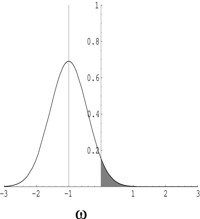
FIG. 1.: Illustration of the bound on $|\tilde{f}^{+}(0)-f^{+}(0)|$, as described in the text. The vertical line describes a $\delta$-function spike in $f(\omega)$. This produces a Gaussian in $\tilde{f}(\omega)$. The integral over $\omega$ of the Gaussian is the same as the integral of the $\delta$-function; however, the shaded region of the curve of the Gaussian falls above $\omega=0$, and hence does not contribute to $f^{+}(0)$. This leads to the difference between $\tilde{f}^{+}(0)$ and $f^{+}(0)$.

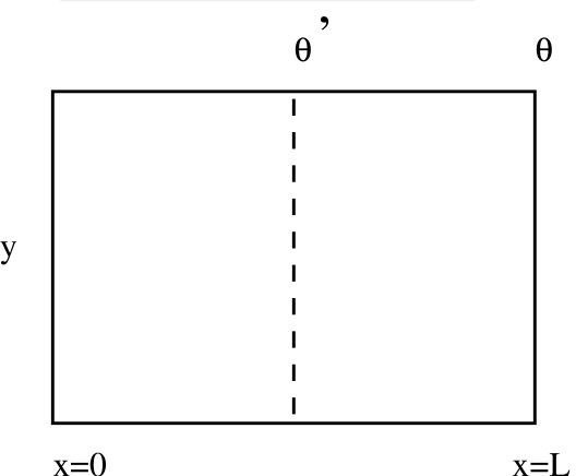
FIG. 2.: Plot of the system, showing the $x$-coordinate along the length axis. The $x$ is shown ranging from $x=0$ to $x=L$; due to the periodicity of the system, $x=0$ is identified with $x=L$. The $y$ coordinate specifies the position in the directions normal to the length, as well as specifying the particular site in each unit cell. The twist angles are noted; the twist $\theta$ changes the boundary condition near $x=L$, while the twist $\theta^{\prime}$ changes the coupling between sites near $x=L/2$.

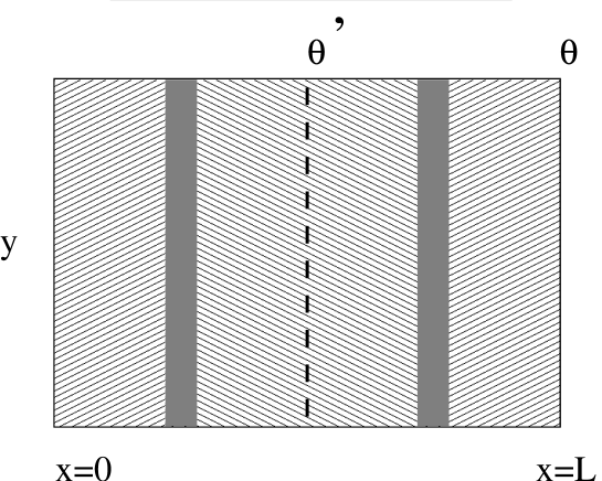
FIG. 3.: Plot of the system, showing the twists and coordinates as before. The halves of the system have been shaded in. The shading at the left and right side of the system (diagonal lines going up and right) denotes sites in half (1), the shading in the middle (diagonal lines going up and left) denotes sites in half (2). The solid shading denotes sites in both halves; the length of the solid region is at least $2R$, so that the Hamiltonian can be written as a sum of terms, each of which is contained in only one half.

REFERENCES

- [1] E. H. Lieb, T. D. Schultz, and D. C. Mattis, Ann. Phys. (N. Y.) 16, 407 (1961).
- [2] F. D. M. Haldane, Phys. Rev. Lett. 50, 1153 (1983).
- [3] I. Affleck, Phys. Rev. B 37, 5186 (1988).
- [4] M. Oshikawa, Phys. Rev. Lett. 84, 1535 (2000).
- [5] G. Misguich, C. Lhuillier, M. Mambrini, and P Sindzingre, Euro. Phys. Jour. B 26, 167 (2002); G. Misguich and C. Lhuillier, cond-mat/0002170.
- [6] B. Sutherland, Phys. Rev. B 37, 3786 (1988); D. Rokhsar and S. Kivelson, Phys. Rev. Lett. 61(1988); N. Read and B. Chakraborty, Phys Rev. B 40, 7133 (1989).
- [7] N. E. Bonesteel, Phys. Rev. B 40, 8954 (1989).
- [8] It follows automatically that Eq. (1) holds for all for some depending on .
- [9] C. K. Majumdar and D. K. Ghosh, J. Math. Phys. 10, 1388 (1969).
- [10] G. Baskaran and P. W. Anderson, Phys. Rev. B 37, 580 (1988).
- [11] I. Affleck and J. B. Marston, Phys. Rev. B 37, 3774 (1988); X. G. Wen, Phys. Rev. B 44, 2664 (1991); N. Read and S. Sachdev, Phys. Rev. Lett. 66. 1773 (1991).
- [12] D. S. Rokhsar and S. A. Kivelson, Phys. Rev. Lett. 61, 2376 (1988); R. Moessner and S. L. Sondhi, Phys. Rev. Lett. 86, 1881 (2001).
- [13] This norm, written , is defined to be the supremum over states , with , of ; R. Bhatia, Matrix Analysis, (Springer-Verlag, New York, 1997).
- [14] E. Lieb and D. Robinson, Commun. Math. Phys. 28, 251 (1972).
- [15] Following standard physics notation, whenever we write we are taking the limit as . The limit is taken outside the integral sign. On the other hand, the use later of is done at a fixed, non-zero value of .
- [16] Eq. (12) follows from contour integration. Another way to derive it is to use a convolution and Fourier transform. Define the Fourier transform of to be (see [17]). Then, . Combining these gives . Doing the integral over gives Eq. (12). Note that is rapidly decaying as , so that there are no issues with convergence.
- [17] Following standard physics notation, in Eq. (18), and throughout, the use of refers to the Fourier transform of The use of always refers to at .
- [18] We note that since we have assumed that the ground state is unique, with a gap , then for any finite , the ground state energy is analytic in in some neighborhood of .
- [19] To show this, consider rotating all the spins by angle about the -axis. Since the ground state is assumed to be unique and the Hamiltonian is invariant under global rotations, the ground state is invariant under global , so that ground state expectation values must be unchanged under this rotation. However, if we take an odd number of derivatives of with respect to , the resulting operator changes sign under a rotation by about the -axis. Therefore, the expectation value of an odd number of derivatives of must vanish.
- [20] Possible low energy topological excitations do not prevent the use of Eq. (22) for spin liquids as the matrix elements of between the ground and topologically excited states are negligible.
- [21] The trace norm of an operator , written , is defined to be . We will deal with Hermitian operators, for which it is equal to the sum of the absolute values of the eigenvalues.
- [22] In fact, need not be differentiable. To get around this, we use the upper derivative[14], defined as .
- [23] We showed before that up to small error is entirely within half (1). For larger , we can in fact ensure that includes only operators within a distance of so that are separated by a distance from each other. Then we can apply the locality bounds to the given correlation function of .
- [24] It turns out that the requirement that the eigenvalues be real is necessary. Although one might have guessed that a similar exponential decay of correlation functions would also hold for complex with real part , there seems to be a counterexample to this statement. This will be discussed in a future publication.