Energy and structure of dilute hard– and soft–sphere gases

Abstract

The energy and structure of dilute hard- and soft-sphere Bose gases are systematically studied in the framework of several many-body approaches, as the variational correlated theory, the Bogoliubov model and the uniform limit approximation, valid in the weak interaction regime. When possible, the results are compared with the exact diffusion Monte Carlo ones. A Jastrow type correlation provides a good description of the systems, both hard- and soft-spheres, if the hypernetted chain energy functional is freely minimized and the resulting Euler equation is solved. The study of the soft-spheres potentials confirms the appearance of a dependence of the energy on the shape of the potential at gas paremeter values of $x\sim 0.001$. For quantities other than the energy, such as the radial distribution functions and the momentum distributions, the dependence appears at any value of $x$. The occurrence of a maximum in the radial distribution function, in the momentum distribution and in the excitation spectrum is a natural effect of the correlations when $x$ increases. The asymptotic behaviors of the functions characterizing the structure of the systems are also investigated. The uniform limit approach results very easy to implement and provides a good description of the soft-sphere gas. Its reliability improves when the interaction weakens.

I Introduction

The study of dilute systems has met a surge of renewed interest in the last years, following the experimental achievement of Bose-Einstein condensation in low density atomic gases confined in harmonic traps. Systems are termed as dilute when the average interparticle distance, $r_{av}$, is much larger than the range of the interaction, $r_{0}$. The main parameter characterizing the interaction in the dilute regime is the $s$–wave scattering length, $a$, and the diluteness condition can be expressed in terms of the density, $\rho$, as $x<<1$, where $x=\rho a^{3}$ is the gas parameter.

Positive values of the scattering length correspond to an essentially repulsive interaction at short distances. In fact, for an infinite repulsive barrier, with no attractive part, $a$ is just given by the radius of the barrier itself. The hard sphere (HS) potential is largely adopted to study low density (LD) gases with positive scattering lengths because of its formal simplicity. However, other potentials, providing the same value of $a$, are indistinguishable from the HS one at very low $x$ (universality property). Additional details of the interaction, giving raise to nonuniversal effects, become relevant when the density (and the gas parameter) increases, allowing for discriminating among different potential shapes. Typical ranges of $x$ where these differences begin to show up have been foundboro99 ; sarsa02 to be $x\geq 10^{-3}$.

In the density ranges attained in Bose-Einstein condensation experiments the local gas parameter may well exceed this value, exploiting the large variation of the scattering length in the vicinity of a Fehsbach resonancecornish00 . In order to quantitatively study this regime it is compulsory to check the reliability of the theories adopted in the analysis. A first, and much needed step in this direction, consists in understanding the properties of the underlying homogeneous gas of bosons at T=0 temperature. This is a time honored subject of many–body physics, addressed by a variety of methods, such as perturbative expansions, Monte Carlo (MC) type samplings, variational theories, and so on.

Expansions in $x$ may be suited to study dilute systems whose interaction can be safely described in terms of the $s$–wave scattering length. They can be derived in the framework of standard perturbation theories, built on the basis constituted by the ground state of a non interacting Bose fluid and its excited states, obtained by promoting particles from the zero momentum condensed state to the non–zero ones. Infinite sums of ladder diagrams must be accomplished for strongly repulsive potentials. This procedure results in the well known Lee and Yang low density expansion for the energy per particle of a homogeneous gas of bosonslee57 ,

$${E\over N}=\left({\hbar^{2}\over{2ma^{2}}}\right)\,4\pi x\,\left[1+{128\over 15}\sqrt{{x\over\pi}}\right]\,.$$ (1)

Low order perturbative diagrams can be retained in the weakly interacting Bose gasfetter characterized by an interaction having a finite Fourier transform.

Alternatively, the interaction may be mimicked in the low density region by a delta–shaped pseudopotentialhuang , related to $a$ by

$$V(r)=4\pi a\hbar^{2}\delta({\bf r})/m\ ,$$ (2)

which reproduces the value of the scattering length in the Born approximation:

$$a_{B}={m\over{4\pi\hbar^{2}}}\int d{\bf r}\,V(r)\,.$$ (3)

This approach is followed in the Bogoliubov theorybogo , by introducing a model hamiltonian containing the pseudopotential. A canonical transformation of the BCS type allows for a partial diagonalization of the model hamiltonian, leading to a $x$–expansion as in (1) for the ground–state energy.

Nonuniversal effects have been studied in effective field theory in Ref.braaten01 , and found to depend, at the leading orders, on the effective range, $r_{s}$, and on a three–body contact force parameter, $c$, determined in this reference by comparison with the exact diffusion Monte Carlo results of Ref.boro99 .

The bosonic many–body Schroedinger equation may be solved, for any potential, by Monte Carlo based methods, as the Green’s Function Monte Carlo and the Diffusion Monte Carlo (DMC) ones. Both approaches are exact, apart from statistical errors, and provide essential benchmarks to test the reliability of other theories, at least in those cases where the numerical accuracy allows for an unbiased analysis of the results.

The variational approach is carried on within the Correlated Basis Functions (CBF) perturbation theory, and represents its zeroth order. The correlated ground state wave function for $N$ interacting particles is obtained by acting with a many–body correlation operator on the non–interacting ground state wave functionfeenberg :

$$\Psi_{0}(1,2,\ldots,N)={\cal F}(1,2,\ldots,N)\Phi_{0}(1,2,\ldots,N)\,.$$ (4)

The operator ${\cal F}(1,2,\ldots,N)$ is meant to take into account the spatial correlations induced by the interaction on the free wave function $\Phi_{0}(1,2,\ldots,N)$ (for homogeneous bosons $\Phi_{0}=1$). For instance, in the HS case the correlation operator prevents the distance between any pair of particles from being smaller than the core radius, so that the wave function vanishes for these configurations. The theory is variational in the sense that ${\cal F}$ is determined by minimizing the ground state energy. A correlated perturbation theory may be constructed by applying the correlation operator to the non–interacting excited states.

The weakly interacting Bose fluid has been recently studied within the variational method by means of the Independent Pair Correlations (IPC) approachsarsa02 . The IPC wave function is written as

$$\Psi_{IPC}(1,2,\ldots,N)=1+\sum_{i<j}h(r_{ij})+{1\over 2}\sum_{(i<j)\neq(l<m)}h(r_{ij})h(r_{lm})+\ldots\,,$$ (5)

where the two–body correlation functions, $h(r)$, always act on non–overlapping, independent pairs. The structure of a Bose system described by the IPC wave function has been analyzed by means of an expansion in cluster diagrams. Renormalized HyperNetted Chain (HNC) integral equations exactly sum all the diagrams and have been used to compute the energy, distribution function, momentum distribution and pairing function of the bulk boson system of soft spheres. The Bogoliubov transformation itself is known to generate a wave function having the IPC structurehuang , and a careful comparison between the variational and Bogoliubov approaches has been performed in Ref.sarsa02 , as well as with the outcomes of the Diffusion Monte Carlo and low density theories, for soft sphere (SS) and gaussian like potentials.

The IPC wave function fails for a hard–sphere fluid, since all pairs need to be simultaneously correlated. This task may be achieved by a Jastrow correlated wave functionfeenberg

$$\Psi_{J}(1,2,\ldots,N)=\prod_{i<j}[1+h(r_{ij})]\,,$$ (6)

where the productory runs over $all$ pairs. The Jastrow ansatz is clearly richer than the IPC one, however it has the disvantage that the HNC equations can be only approximately solved, since a class of diagrams (the $elementary$ diagrams) is not summable in a closed wayHNC . The approximations in the solution of the Jastrow–HNC equations are not expected to be quantitatively relevant in the low density regime, however the computed energy is, in principle, no longer a rigorous upperbound to the true one, in contrast with the IPC case.

In this paper we consider a system of $N$ spinless bosons of mass $m$ in a volume $\Omega$, described by the hamiltonian

$$H=-{\hbar^{2}\over 2m}\sum_{j=1}^{N}\nabla^{2}_{j}+\sum_{1=i<j}^{N}V(r_{ij})\,$$ (7)

where $V(r)$ is a two-body, spherically symmetric potential, in the thermodynamic limit ( $N$ and $\Omega$ $\rightarrow\infty$, keeping the density, $\rho=N/\Omega$, constant).

Two different representative choices for the potential are studied: the hard-sphere potential,

$$V(r)=\left\{\begin{array}[]{ll}\infty&\,\,\,\,\,r<a\\ 0&\,\,\,\,\,r>a\ ,\end{array}\right.$$ (8)

where the diameter $a$ of the hard sphere coincides with the $s$–wave scattering length, and a soft sphere potential,

$$V(r)=\left\{\begin{array}[]{ll}V_{0}>0&\,\,\,\,\,r<R\\ 0&\,\,\,\,\,r>R\ ,\end{array}\right.$$ (9)

whose $s$-wave scattering length is given by

$$a=R\left[1-\tanh(K_{0}R)/(K_{0}R)\right],$$ (10)

with $K_{0}^{2}=V_{0}m/\hbar^{2}$.

The $optimal$ Jastrow correlated wave function, obtained by the minimization of the energy per particle through the solution of the HNC Euler equation kro98 , is used along this work. We compute the radial distribution function, $g(r)$, the static structure function, $S(k)$, and the momentum distribution, $n(k)$, for HS and SS models with identical scattering lengths, to ascertain the dependence on the potential form along the gas parameter. We work in the HNC/0 approximation, which amounts to disregard the contribution from the elementary diagrams and whose accuracy is tested by comparison with the exact DMC results. Moreover, the Jastrow theory is compared with the LD expansion and with the Bogoliubov and IPC theories for the SS case. In addition, the SS potential is examined in the so called uniform limit (UL)feenberg , defined by assuming $|g(r)-1|<<1$ for all $r$. Special emphasis is devoted to the analysis of several asymptotic behaviors. This is an interesting issue that cannot be fully addressed with DMC methods, since the limited size of the simulation box strongly limits the possibility of studying effects related to long range structures.

The plan of the paper is as follows: the HNC/0 and Euler equations are shortly revisited in Section II; the uniform limit for the SS potential and its connection with the Random Phase Approximation (RPA) theory are discussed in Section III; Section IV present the results for the HS and SS models and summary and conclusions are given in Section V.

II HNC theory

The exact wave function of a homogenous, interacting Bose system can be written as the product of up to $N$–body correlation factorsfeenberg

$$\Psi_{0}(1,2,\ldots,N)=\prod_{i<j}^{N}f_{2}(r_{ij})\prod_{k<l<m}^{N}f_{3}({\bf r}_{kl},{\bf r}_{km},{\bf r}_{lm})\cdots\ ,$$ (11)

where $r_{ij}=\mid{\bf r}_{i}-{\bf r}_{j}\mid$ and $f_{n}>0$ for all $n$. High density and strongly interacting systems, like atomic liquid ⁴He, are accurately described by keeping only two– and three–body correlations ($f_{n>3}=1$). Moreover, a proper choice of $f_{2}$ already contributes by $\sim 70\%$ to the ⁴He energyHNC . So, for weak interactions and/or low density fluids, the simpler Jastrow correlated wave function of Eq.(6) may largely be enough to capture the essential features of the exact ground state and to provide a quantitatively correct description.

II.1 Radial distribution function and Euler equation

The optimal Jastrow correlation function is obtained by minimizing, without restrictions, the expectation value of the hamiltonian (7), giving the ground state energy,

$$E[f_{2}]={\left\langle\Psi_{0}\mid H\mid\Psi_{0}\right\rangle\over\left\langle\Psi_{0}\mid\Psi_{0}\right\rangle}\,.$$ (12)

This is accomplished by solving the Euler–Lagrange equation camp

$${\delta E[f_{2}]\over\delta f_{2}(r)}=0\,.$$ (13)

The link between the energy and $f_{2}$ is provided by the radial distribution function, $g(r)$,

$$g(r_{12})={{N(N-1)}\over\rho^{2}}{{\int d{\bf r}_{3}d{\bf r}_{4}\ldots d{\bf r}_{N}|\Psi_{0}|^{2}}\over{\int d{\bf r}_{1}d{\bf r}_{2}\ldots d{\bf r}_{N}|\Psi_{0}|^{2}}}\,,$$ (14)

as, in fact,

$${E\over N}=\frac{1}{2}\rho\int d{\bf r}_{12}\,g(r_{12})\,\left[V(r_{12})-\frac{\hbar^{2}}{2m}\nabla^{2}\ln f_{2}(r_{12})\right]\ .$$ (15)

The Jackson–Feenberg identityfeenberg has been used to derive Eq.(15). In turn, the radial distribution function can be computed by solving the HyperNetted Chain equations:

$$g(r_{12}) = f_{2}^{2}(r_{12})\,e^{N(r_{12})+E(r_{12})}$$

$$N(r_{12}) = \rho\int d{\bf r}_{3}[g(r_{13})-1][g(r_{32})-1-N(r_{32})]\,,$$ (16)

where $N(r)$ and $E(r)$ are the sum of the nodal and elementary diagrams, respectivelyHNC . The function $E(r)$ is an input to the theory, and the solution of the HNC equations depends on its choice. In the HNC/0 scheme this function is set to be zero. This seemingly drastic approximation is, however, reliable at low densities since the diagrams contributing to $E(r)$, being highly interconnected, are relevant mostly in the large density regions.

By inverting the relations (16) it is possible to express the energy as a functional of the radial distribution function, and formally rewrite the Euler equation as:

$${\delta E[g]\over\delta g(r)}=0\,.$$ (17)

If this procedure is carried on in $r$–space, the outcome is an integro–differential equation for $g(r)$HNC . Alternatively, the energy can be written in terms of the static structure function, $S(k)$, defined as the Fourier transform of the radial distribution function,

$$S(k)=1+\rho\int d{\bf r}\,e^{i{\bf k}\cdot{\bf r}}(g(r)-1)\ .$$ (18)

Variation of $E[S]$ leads to the equationskro98 :

$$S(k)={t(k)\over\sqrt{t^{2}(k)+2V_{ph}(k)t(k)}}\ ,$$ (19)

with $t(k)=\hbar^{2}k^{2}/2m$ and $V_{ph}(k)$ the so called particle–hole interaction. In $r$–space and in HNC/0,

$$V_{ph}(r)=g(r)V(r)+{\hbar^{2}\over m}\left|\nabla\sqrt{g(r)}\right|^{2}+\left[g(r)-1\right]\omega_{I}(r)\ ,$$ (20)

where the $k$–space induced interaction, $\omega_{I}(k)$, is

$$\omega_{I}(k)=-{1\over 2}t(k){\left(2S(k)+1\right)\left(S(k)-1\right)^{2}\over S^{2}(k)}\ .$$ (21)

Eqs.(19), (20) and (21) are a set of nonlinear coupled equations to be solved iteratively. Finally, the knowledge of $S(k)$ (or $g(r)$) allows to find the optimal Jastrow correlation function by inversion of the HNC/0 equations.

In the HS model the Euler formalism simplifies, since $V_{ph}(r<a)=-\omega_{I}(r)$ and $V_{ph}(r>a)=\hbar^{2}/m\left|\nabla\sqrt{g(r)}\right|^{2}+[g(r)-1]\omega_{I}(r)$.

II.2 Momentum distribution

The one–body density matrix for an homogeneous Bose fluid,

$$\rho_{1}({\bf r}_{1},{\bf r}_{1^{\prime}})=\rho_{1}(r_{11^{\prime}})=N{\int d{\bf r}_{2}d{\bf r}_{3}\cdots d{\bf r}_{N}\Psi_{0}(1,2,\ldots,N)\Psi_{0}(1^{\prime},2,\ldots,N)\over\int d{\bf r}_{1}\cdots d{\bf r}_{N}|\Psi_{0}|^{2}}\ ,$$ (22)

contains essential information about the depletion of the condensate in interacting systems and the consequent finite occupation of single particle states carrying non–zero momentum. Its diagonal part coincides with the one–body density, and in an homogeneous system $\rho_{1}(r=0)=\rho$. The condensate fraction, $n_{0}$, ($i.e.$ the fractional occupation of the $k=0$ momentum state) is related to the long range order of the one–body density matrix by: $n_{0}=\rho_{1}(r\rightarrow\infty)/\rho$.

The associated momentum distribution, $n(k)$, is obtained through the Fourier transform of the one–body density matrix,

$$n(k)=(2\pi)^{3}\rho n_{0}\delta({\bf k})+\int d{\bf r}\,\exp{(i{\bf k}\cdot{\bf r})}\,[\rho_{1}(r)-\rho n_{0}]\,.$$ (23)

The momentum distribution is normalized as

$$1={1\over(2\pi)^{3}\rho}\int d{\bf k}\,n(k)\ ,$$ (24)

while the kinetic energy per particle can be obtained by $n(k)$ through

$${T\over N}={1\over(2\pi)^{3}\rho}\int d{\bf k}\,{\hbar^{2}k^{2}\over 2m}\,n(k)\ .$$ (25)

The HNC/0 scheme has been extended to evaluate the one–body density matrix for a Jastrow correlated wave functionfantoni78 . As a consequence, one gets

$${{\rho_{1}(r)}\over\rho}=n_{0}\,e^{N_{ww}(r)}\ ,$$ (26)

where the new nodal function, $N_{ww}(r)$, is given by

$$N_{ww}(r_{12})=\rho\int d{\bf r}_{3}[g_{wd}(r_{13})-1][g_{dw}(r_{32})-1-N_{dw}(r_{32})]\,.$$ (27)

In the HNC/0 scheme, the functions $g_{wd}$ and $N_{wd}$ are solutions of the set of coupled equations

$$g_{wd}(r) = f(r)\,e^{N_{wd}(r)}$$

$$N_{wd}(r_{12}) = \rho\int d{\bf r}_{3}[g_{wd}(r_{13})-1][g(r_{32})-1-N(r_{32})]\,,$$ (28)

with $g_{wd}(r_{12})=g_{dw}(r_{21})$ and $N_{wd}(r_{12})=N_{dw}(r_{21})$.

The condensate fraction, $n_{0}$, is given in terms of the vertex factors, $R_{w}$ and $R_{d}$, as

$$n_{0}=e^{2R_{w}-R_{d}}\ ,$$ (29)

where

$$R_{w}=\rho\int d{\bf r}\,[g_{wd}(r)-1-N_{wd}(r)]-{\rho\over 2}\int d{\bf r}\,[g_{wd}(r)-1]\,N_{wd}(r)\,,$$ (30)

and $R_{d}$ is obtained by substituting in (30) $g_{wd}\rightarrow g$ and $N_{wd}\rightarrow N$.

III Soft spheres in the uniform limit approximation

The formalism presented in the previous section is independent on the shape of the potential. Hence it is equally well suited to analyze both HS and SS systems. However, everywhere bounded potentials, as the SS one, allow for alternative calculations complementing the HNC results. A simple estimate of the energy, in this case, is provided by first order perturbation theory, which yields an upper–bound to the exact ground state energy:

$$\frac{E_{1}(\rho)}{N}=\frac{\langle\Phi_{0}\mid H\mid\Phi_{0}\rangle}{N}=\frac{1}{2}\rho V_{0}\frac{4}{3}\pi R^{3}=\frac{1}{2}\tilde{V}(0)\ ,$$ (31)

where $\tilde{V}$ is the Fourier transform of the potential and $\phi_{0}=1/\Omega^{N/2}$ is the wave function of the corresponding free system, with all particles occupying the zero momentum state. The second order perturbative correction to the energy is also easily obtained as

$$\frac{E_{2}(\rho)}{N}=-\frac{1}{2\rho}\int{d{\bf q}\over(2\pi)^{3}}{\mid\tilde{V}(q)\mid^{2}\over\hbar^{2}q^{2}/m}\ ,$$ (32)

however the resulting total energy $E(\rho)=E_{1}(\rho)+E_{2}(\rho)$ is no longer a bound to the exact one.

If the interaction is finite the uniform limit approximationfeenberg may also give an accurate description of a dilute system. In this regime, correlations are assumed to be weak and the ground state is only slightly affected by them. This condition reads, in terms of the radial distribution function, as $|g(r)-1|<<1$, as already mentioned in the Introduction. In the uniform limit the HNC energy simplifies as:

$$\frac{E_{UL}(\rho)}{N}=\frac{1}{2}\tilde{V}(0)+\frac{1}{2}\int{d{\bf k}\over(2\pi)^{3}\rho}\left[(S(k)-1)\tilde{V}(k)+\frac{\hbar^{2}k^{2}}{4m}\frac{(S(k)-1)^{2}}{S(k)}\right]\ ,$$ (33)

an expression that can be readily obtained from Eq. (15) by assuming $g(r)\sim 1$, so that $\ln g(r)\approx g(r)-1$. The last term in the integral is the kinetic energy contribution, and by comparing it with (25) one readily realizes that the momentum distribution is related to the static structure function in the UL through the relation:

$$n(k)=\frac{(S(k)-1)^{2}}{4S(k)}\ .$$ (34)

The condensate fraction, $n_{0}$, can then be recovered by imposing the normalization condition (24).

Minimization of $E_{UL}$ with respect to $S(k)$ gives the Euler-Lagrange equation in the UL,

$$\tilde{V}(k)+\frac{\hbar^{2}k^{2}}{4m}{(S^{2}(k)-1)\over S^{2}(k)}=0\ ,$$ (35)

which can be solved for the the static structure function to obtain:

$$S_{UL}(k)=\frac{t(k)}{\sqrt{t^{2}(k)+2t(k)\tilde{V}(k)}}\ .$$ (36)

This expression is formally identical to the HNC one of Eq. (19), where $V_{ph}(k)$ has been approximated by the Fourier transform of the bare potential $V(r)$.

We notice that $S_{UL}(k)$ coincides with the static sturcture function given by the RPA approximation to the dynamic susceptibility, $\chi(k,\omega)$ kro98 ,

$$\chi_{RPA}(k,\omega)=\frac{\chi_{0}(k,\omega)}{1-\tilde{V}(k)\chi_{0}(k,\omega)}\ ,$$ (37)

where $\chi_{0}(k,\omega)$ is the dynamic susceptibility of the free Bose gas at zero temperature,

$$\chi_{0}(k,\omega)=\frac{1}{\omega-t(k)+i\epsilon}-\frac{1}{\omega+t(k)+i\epsilon}\ .$$ (38)

The poles of $\chi_{RPA}(k,\omega)$, $\epsilon_{RPA}(k)=\left(t(k)^{2}+2t(k)\tilde{V}(k)\right)^{1/2}$, define the excitation energies of the system, while the imaginary part of $\chi_{RPA}(k,\omega)$ gives the dynamic structure function,

$$S_{RPA}(k,\omega)=-\frac{1}{\pi}\Im\chi_{RPA}(k,\omega)=\frac{t(k)}{\epsilon_{RPA}(k)}\delta(\omega-\epsilon_{RPA}(k))\ .$$ (39)

Integration of $S_{RPA}(k,\omega)$ over $\omega$ leads to the static structure function, $S_{RPA}(k)$,

$$S_{RPA}(k)={t(k)\over\sqrt{t^{2}(k)+2t(k)\tilde{V}(k)}}\ ,$$ (40)

which coincides with $S_{UL}(k)$. Moreover, the UL energy (33) can be obtained by adding the RPA correction, $\triangle E_{RPA}$, to the uncorrelated energy (31). $\triangle E_{RPA}$ can be evaluated by performing a coupling constant integration,

$$\triangle E_{RPA}={\frac{1}{2}}\int{d{\bf k}\over(2\pi)^{3}\rho}\,\tilde{V}(k)\int_{0}^{1}\left[S_{\lambda}(k)-1\right]d\lambda\ ,$$ (41)

$S_{\lambda}(k)$ being the RPA static structure function corresponding to the interaction $\lambda\tilde{V}(k)$. After a straigthforward integration the uniform limit expression is recovered,

$$E_{UL}=\frac{1}{2}\tilde{V}(0)+\triangle E_{RPA}\ .$$ (42)

A similar result has been found in Ref.sarsa02 , where the soft-sphere gas has been studied in the framework of the HNC theory with an independent pair correlated wave function. The authors have shown that neglecting the composite diagrams and summing the chain diagrams only, the HNC/IPC approach leads to the RPA (and UL) energy functional (33). All three theories produce the same description of the soft-sphere gas in the low density regime, since both uniform limit and correlated theories, in conjuction with a proper minimization via the Euler equation, take into account the long range correlations relevant in this region and correctly considered by the RPA.

III.1 Some aspects of the low density expansion

The formalism outlined in Section II allows to describe the ground state of any boson liquid or gas characterized by a hamiltonian of the form given in (7). At very low densities, however, all interacting Bose gases having the same scattering length are expected to behave in a similar way, as originally pointed out by Bogoliubov bogo . The energy of a Bose gas follows the universal form (1) as long as the system is dilute. However, the overall energy comes from a balance between kinetic and potential contributions. For hard spheres the energy is entirely kinetic, whereas for soft spheres the relative contribution of the potential energy may be as large as possible, according to the softness of the interaction.

Despite the universality exhibited by the total energy, it is not clear that other ground state properties may show an analogous behavior. An answer to this question can be obtained by analyzing the hard and soft sphere gases and comparing with the predictions obtained within the Bogoliubov model. For instance, from the Bogoliubov excitation spectrum,

$$\epsilon_{B}(k)=\sqrt{t^{2}(k)+2t(k)4\pi a\hbar^{2}\rho/m}\ ,$$ (43)

an approximate static structure factor can be obtained assuming a Feynman–like spectrum,

$$S_{B}(k)={t(k)\over\epsilon_{B}(k)}\ .$$ (44)

However, $g(r)$ extracted from $S_{B}(k)$ is unphysically divergent at $r=0$.

In the Bogoliubov model the momentum distribution, $n_{B}(k)$, at $k>0$ can be written in the formhuang :

$$n_{B}(k)={A_{k}^{2}\over 1-A_{k}^{2}}\,\,\,\,\,,\,\,\,\,\,A_{k}=1+{m\over 4\pi a\hbar^{2}\rho}\left[t(k)-\epsilon_{B}(k)\right]\ .$$ (45)

This expression coincides with $n(k)$ as obtained in the UL (Eq.(34)) when $\tilde{V}(k)$ is replaced by $4\pi a\rho\hbar^{2}/m$.

Normalization of the full momentum distribution gives the fraction of particles in the $k=0$ state, $n_{0B}$,

$$n_{0B}=1-{8\over 3}\sqrt{x\over\pi}\ .$$ (46)

The kinetic energy computed through $n_{B}(k)$ is divergent since $n_{B}(k)\sim k^{-4}$ at large $k$.

IV Dilute hard spheres

In this section variational results for the energy, two-body distribution function, static structure function and one-body density matrix (and momentum distribution) of a dilute gas of hard spheres are shown and discussed. The driving quantity of any variational approach is the total energy, given by the sum of the kinetic and potential terms. Since inside the core of the potential $g(r)=0$, the energy is purely kinetic and, in units of $\hbar^{2}/2ma^{2}$, becomes

$$\frac{{\bar{E}}(x)}{N}=\frac{\langle{\bar{T}}\rangle}{N}=-{1\over 2}x\int d{\bf r}\,g(r)\nabla^{2}\ln f(r)\ .$$ (47)

We will adopt the long ranged correlation function obtained by solving the Euler–Lagrange equations and will analyze the related asymptotic behaviors. However, the HNC results for a simpler correlation function having a short–range structure, $f_{SR}(r)$, are also discussed. $f_{SR}(r)$ is choosen in such a way to minimize the lowest–order in the cluster expansion of the energy of the homogeneous gas of HS with a healing condition at a distance $d$, taken as a variational parameterfSR . In the HS case $f_{SR}(r)$ is:

$$f_{SR}(r)=\left\{\begin{array}[]{ll}0&\,\,\,\,\,r<1\\ {d\over r}{\sin[K(r-1)]\over\sin[K(d-1)]}&\,\,\,\,\,r>1\ ,\end{array}\right.$$ (48)

where distances are in units of $a$ and $K$ fulfills the equation: $cot[K(d-1)]=(Kd)^{-1}$. The latter condition ensures the healing properties: $f_{SR}(r\geq 1)=1$ and $f^{\prime}_{SR}(r=d)=0$.

The scaled energies per particle, ${\bar{E}}(x)/N$, of the HS gas as a function of the gas parameter, $x$, are given in Table 1. ${\bar{E}}_{EL}$ is obtained by solving the Euler-Lagrange equation, while in computing ${\bar{E}}_{SR}$ the short–range correlation (48) has been used. Both energies are computed within the HNC/0 approximation, justified a priori by the smallness of $x$, and a posteriori by the eventual agreement with the exact DMC resultsboro99 , reported also in the Table together with the results of the LD expansion (1).

${\bar{E}}_{EL}$ and ${\bar{E}}_{SR}$ are upper bounds to the exact DMC energy. Furthermore, since the solution of the Euler–Lagrange equations yields the minimum energy for a Jastrow type wave function, the inequality ${\bar{E}}_{DMC}\leq{\bar{E}}_{EL}\leq{\bar{E}}_{SR}$ holds at each density. Violations of this hiearchy at low $x$–values are probably due to numerical inaccuracies, rather than to the HNC/0 approximation.

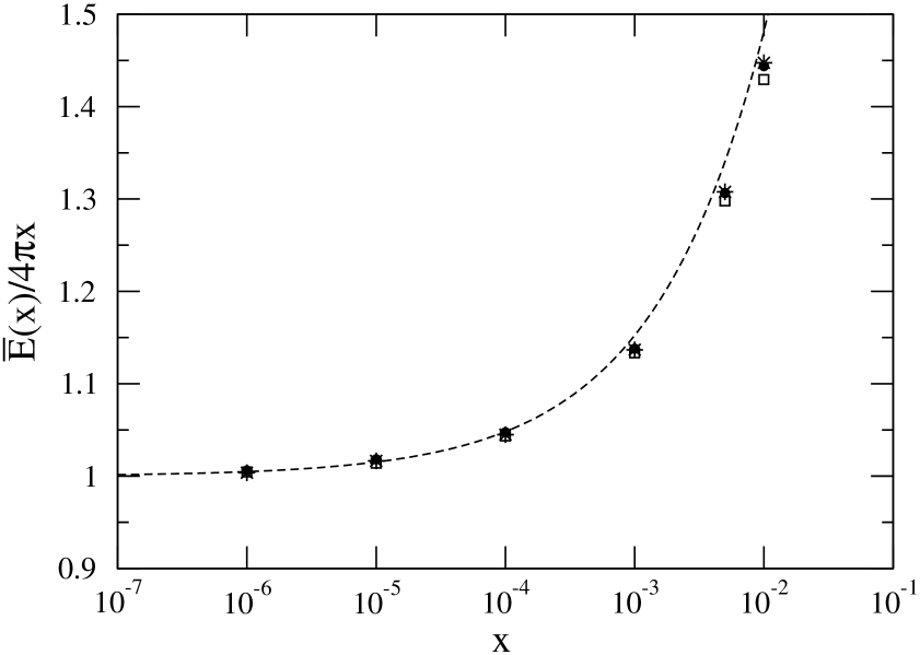
Figure 1: Scaled energy per particle of the HS gas as a function of $x$. Solid circles: Euler–Lagrange results; stars: HNC/0 results for the parametrized two–body correlation factor of Eq.(48); open squares: Diffusion Monte Carlo resuls; dashed line: first two terms of the low density expansion, Eq.(1).

The low-density expansion does not satisfy the upper bound property. However, the lowest order of the same expansion, ${\bar{E}}_{LD0}/N=4\pi x$, is a rigorous lower bound to the exact energy lieb1 . The overall differences among the EL, SR and DMC energies are very small (at most $6\%$ in the worst case at $x=0.1$) and both the EL and the SR results can be taken as good estimates. Using the HNC/0 scheme is therefore well justified in the range of densities explored, especially at the lowest ones. For the sake of comparison, a Variational Monte Carlo (VMC) calculation at $x=0.1$, with $f_{SR}(r)$ having a healing distance $d=6$, has also been carried out in order to estimate the relevance of the elementary diagrams. The result ${\bar{E}}_{VMC}/N=3.74\pm 0.02$ is to be compared with ${\bar{E}}_{SR}/N=3.97$ in HNC/0. Hence, at the highest density considered the elementary diagrams contribute by only $\sim 6\%$ to the energy. Further differences with the DMC results have to be attributed to deficiencies in the two–body correlation factor and to the lack of three- and higher body correlations in the trial wave function. The energies in these approximations are plotted in Fig. 1, where the subtle differences between the points are hardly appreciable, except at the highest $x$’s.

The influence of the optimization on the energy is rather small. The energy is dominated by the short range structure of the potential, which requires the two body distribution function to be zero inside the hard core. The Euler–Lagrange procedure is instead important in establishing the long range structure of the distribution function $g(r)$, or, alternativeley, of the low $k$ behavior of $S(k)$.

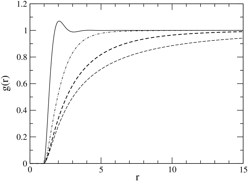
Figure 2: EL radial distribution function $g(r)$ for HS at $x=10^{-4}$ (short-dashed line), $x=10^{-3}$ (long-dashed line), $x=10^{-2}$ (dot-dashed line) and $x=10^{-1}$ (solid line). Distances in units of $a$.

The $EL$ radial distribution function is shown in Fig. 2 for several values of the gas parameter. At low $x$’s $g(r)$ is a monotonically increasing function of the distance, approaching faster and faster the asymptotic limit, $g(r)\to 1$, with the density. This behavior is readily understood recalling that $g(r)$ measures the probability of finding two particles at a distance $r$, and the average interatomic spacing decreases with the density. At large densities the radial distribution function develops a local maximum close to the core radius.

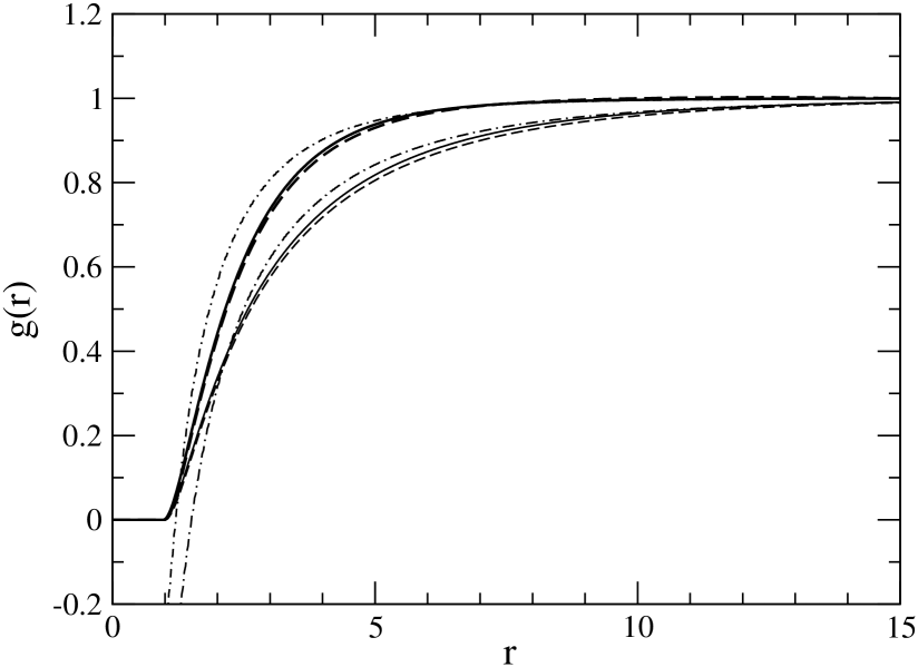
Figure 3: EL (solid lines), SR (dashed lines) and Bogoliubov (dash–dotted lines) radial distribution functions for HS. Upper and lower curves correspond to $x=0.005$ and $x=0.001$, respectively. Distances in units of $a$.

The radial distribution functions, $g_{EL}(r)$, solutions of the EL equation at $x=0.001$ and $x=0.005$, are compared in Fig. 3 with the corresponding short-range ones, $g_{SR}(r)$, computed from $f_{SR}(r)$. At these densities, the energy of the system is accurately described by the expansion of Eq. (1), and it is natural to compare other ground state quantities to those corresponding to the Bogoliubov approximation. Fig. 3 also shows the radial distribution function, $g_{B}(r)$, obtained as the Fourier transform of $S_{B}(k)$,

$$S_{B}(k)={k^{2}\over\sqrt{k^{4}+16\pi xk^{2}}}\ .$$ (49)

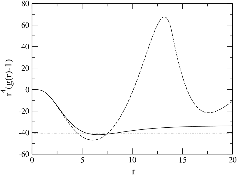
Figure 4: Long range structure of the HS $g(r)$ at $x=0.005$ in the EL (solid line), SR (dashed line) cases compared with the $r\rightarrow\infty$ contribution in the Bogoliubov approximation (dot–dashed line). Distances in units of $a$.

$g_{EL}(r)$ and $g_{SR}(r)$ are close at short distances: they both vanish inside the core and approach similarly the unity. However, differences with $g_{B}(r)$ are significant. $g_{B}(r)$ becomes unphysically negative at short distances to finally diverge at $r\to 0$. In fact, $S_{B}(k)$ realistically reproduces only the low $k$ behavior of the static structure function in dilute systems. This corresponds to the large–$r$ region in the associated radial distribution function. For the same reason, $g_{B}(r)$ never develops a maximum. The three radial distribution functions have different asymptotic behaviors, as shown in Fig. 4, where $r^{4}(g(r)-1)$ is given in the EL, SR and Bogoliubov approaches at $x=0.005$. Both $g_{EL}(r)-1$ and $g_{B}(r)-1$ behave as $r^{-4}$ at large $r$, a property not shown by $g_{SR}(r)-1$ since $f_{SR}(r)$ does not have the appropriate long range behavior, $f(r\to\infty)-1\sim r^{-2}$. Actually, the long range behavior of $g(r)$ is related to the sound velocity, $c$ (in units of $\hbar/2ma$), byfeenberg

$$g(r\to\infty)\sim 1-\frac{1}{\pi^{2}cx}\frac{1}{r^{4}}\ ,$$ (50)

and consequently, the static sturcture function goes like

$$S(k\to 0)\to{k\over c}\ .$$ (51)

In the Bogoliubov approximation,

$$g_{B}(r\to\infty)\sim 1-\frac{1}{4\pi^{5/2}x^{3/2}}\frac{1}{r^{4}}\ ,$$ (52)

and $c_{B}=\sqrt{16\pi x}$, consistent with the value provided by the compressibility, $\kappa_{T}$, $c=(\rho m\kappa_{T})^{-1/2}/(\hbar/2ma)$, by keeping only the first term in the low-density expansion of the energy. At $x=0.005$ the constant value of $r^{4}(g_{B}(r)-1)=-40.4$ gives $c_{B}=0.50$, smaller than the estimated $c_{EL}=0.61$.

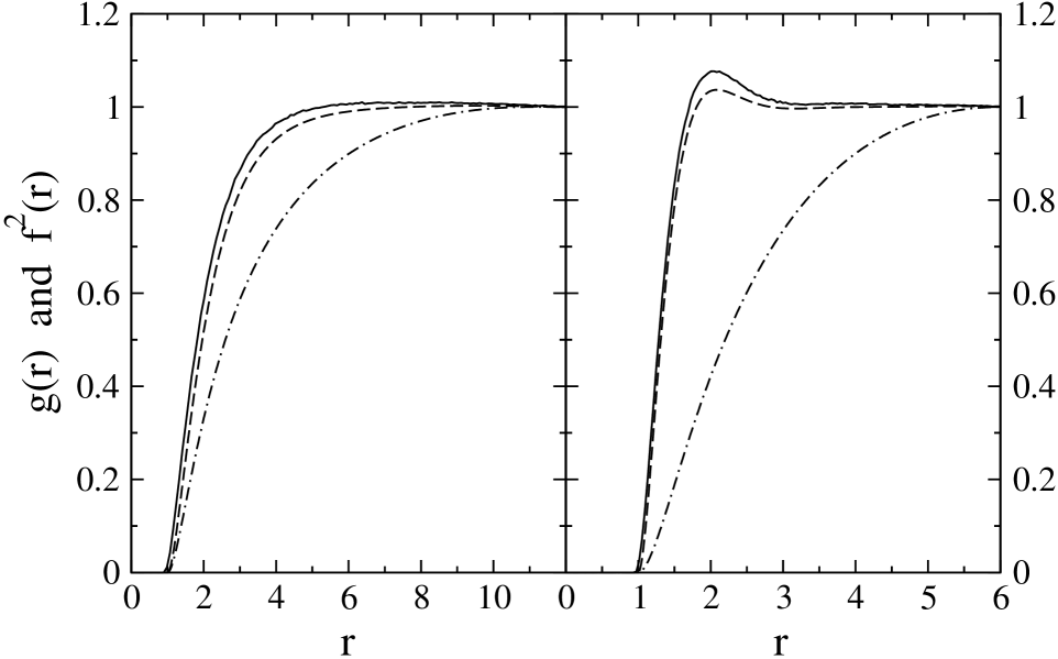
Figure 5: $g_{VMC}(r)$ (solid line) and $g_{HNC/0}(r)$ (dashed line) computed from $f^{2}_{SR}(r)$ of Eq.(48) (dot–dashed line) for HS at $x=0.01$ (left panel) and $x=0.1$ (right panel). Distances in units of $a$.

The short-range radial distribution function is compared in Fig. 5 with the VMC one at $x=0.01$ and $0.1$, for the same two–body correlation factor. We notice two aspects: ($i$) the inclusion of the elementary diagrams enhances the peak of the radial distribution function, and ($ii$) there is a remarkable difference between $f_{SR}^{2}(r)$ and $g(r)$. The many-body contributions included by the HNC scheme cannot be neglected and, therefore, $g(r)$ cannot be approximated by its lowest order cluster expansion value, $g_{LO}(r)=f^{2}(r)$.

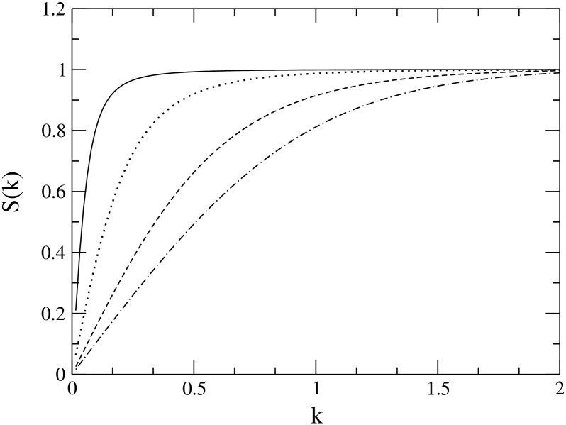
Figure 6: HS EL static structure factor $S(k)$ at $x=10^{-4}$ (solid line), $x=10^{-3}$ (dotted line), $x=5\cdot 10^{-3}$ (dashed line) and $x=10^{-2}$ (dot–dashed line). Momenta in units of $a^{-1}$.

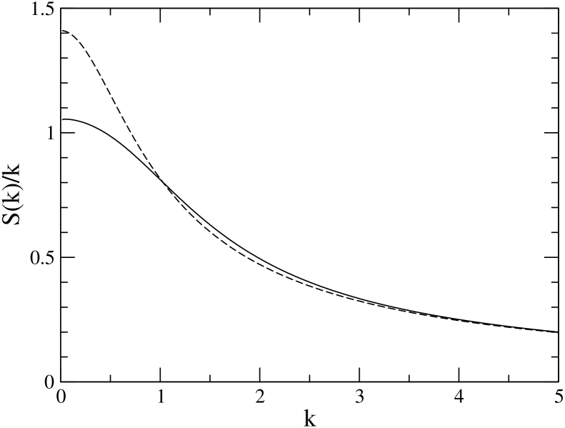
Figure 7: HS $S(k)/k$ in the EL (solid line) and Bogoliubov (dashed line) cases at $x=0.01$. Momenta in units of $a^{-1}$.

The optimal structure function $S(k)$ is shown for several values of $x$ in Fig. 6. The slope of $S(k)$ becomes smaller when $x$ increases because the speed of sound increases with the density. Furthermore, the linear low $k$ behavior, which guarantees the correct low energy excitation spectrum, is evident. However, the linearity of the static structure holds only at very low $k$, as can be seen from Fig. 7, where the ratio $S(k)/k$ is shown in both the EL and the Bogoliubov cases at $x=0.01$. In the later case the linear regime is valid only when $k\ll\sqrt{16\pi x}=c_{B}$ (see Eq.(49)).

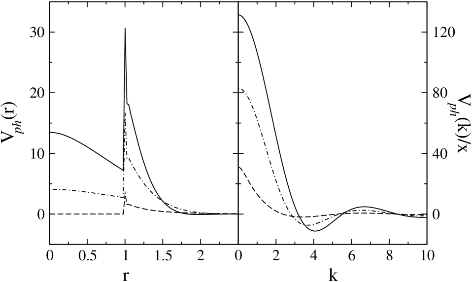
Figure 8: EL Particle–Hole interaction of the HS gas at $x=0.1$ (solid line), $x=0.05$ (dot-dashed line) and $x=0.001$ (dashed line). Distances in units of $a$ and momenta in units of $a^{-1}$.

The particle-hole interaction $V_{ph}$ (Eq. (20)), is shown in Fig. 8 for $x=0.001$, $x=0.05$ and $x=0.1$. The left panel gives $V_{ph}$ in $r$–space. Two regions are separated by a discontinuity at $r=1$, produced by the term $\mid\nabla\sqrt{g(r)}\mid^{2}$ in Eq. (20) since the first derivative of the HS radial distribution function is discontinuous at the core. As already noticed, $-V_{ph}(r<1)$ coincides with the induced interaction, $\omega_{I}(r)$ (21). At the lowest densities $\mid\nabla\sqrt{g(r)}\mid^{2}$ dominates and the strength of $V_{ph}(r)$ is almost entirely exhausted by it. The right panel displays the Fourier transform of $V_{ph}$ at the same densities. $V_{ph}(k)$ is an oscillating function of $k$, with its highest amplitude at $k=0$, and $V_{ph}(k=0)=c^{2}/2$. Notice that the figure shows $V_{ph}(k)/x$, therefore $V_{ph,B}(k)/x$ would be $8\pi$ constant and independent of $k$ and $x$, which turns out to be a very bad approximation to $V_{ph}(k)/x$. However calculating the speed of sound from the two terms of Eq. (1), one gets $c^{2}/2x=8\pi+128\pi^{1/2}x^{1/2}$, in much better agreement with EL $V_{ph}(k=0)/x$.

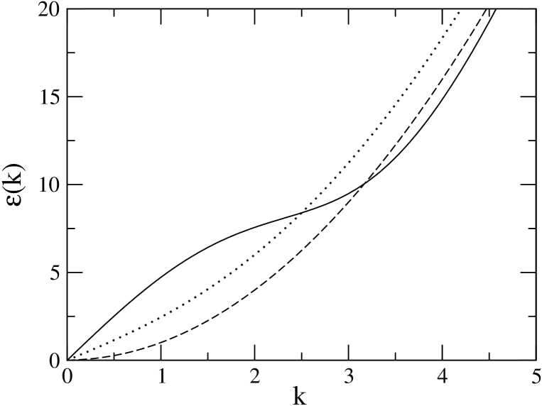
Figure 9: Excitation spectrum of the HS gas. Solid line: EL at $x=0.1$, dotted line: Bogoliubov at $x=0.1$, dashed line: EL at $x=0.001$. Momenta in units of $a^{-1}$.

The Bogoliubov estimate of the particle–hole interaction (Eqs.(19) and (49)) is $V_{ph,B}(k)=8\pi x$ and it is a rather poor approximation to $V_{ph}(k)$. In this case, the excitation spectrum, $\epsilon(k)=t(k)/S(k)\equiv\sqrt{k^{4}+2k^{2}V_{ph}(k)}$, does never develop a rotonic structure, since $V_{ph,B}(k)$ is a constant. In the EL approach, instead, the first oscillations of $V_{ph}(k)$ (and of the static structure function) are large enough to produce a maxon–roton behavior at the largest $x$ value ($x=0.1$). The two spectra are explicitely shown in Fig. 9. The Figure also gives $\epsilon(k)$ at $x=0.001$, where the differences between the EL and Bogoliubov results can hardly be resolved.

The last quantity analyzed is the momentum distribution, $n(k)$. Table 2 reports the condensate fraction, $n_{0}$, and the kinetic energy for both the EL and the SR correlation factors. The Table gives the kinetic energies estimated by Eq. (25), $T_{n}$, and by the second term of Eq. (15), $T_{g}$. At low $x$ values the two estimates almost coincide, whereas, discrepancies at larger densities are to be ascribed to the lack of the elementary diagrams contribution in the cluster expansions of the radial distribution function and the momentum distribution. It has to be noticed that these diagrams play different roles in the two expansionsfantoni78 .

The condensate fraction decreases with $x$, running from $\sim 95\%$ at $x=0.001$ to $\sim 33\%$ for $x=0.08$. The corresponding predictions for $n_{0B}$ (Eq.46) are $n_{0B}(x=0.001)=0.95$ and $n_{0B}(x=0.08)=0.57$. This points again to the failure of the Bogoliubov model at large densities.

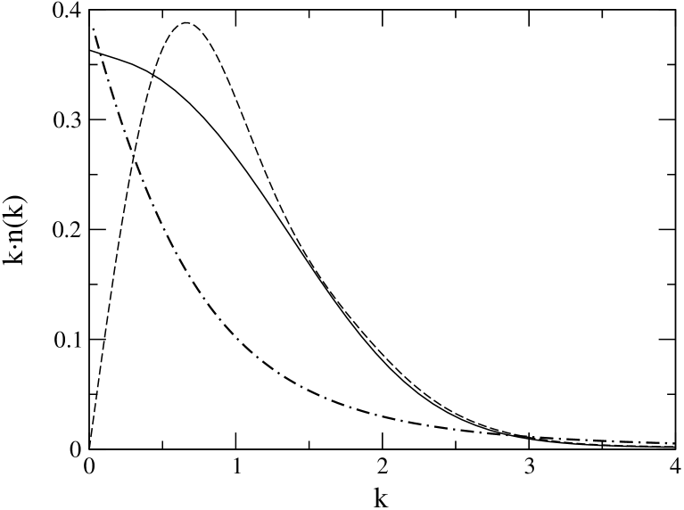
Figure 10: HS momentum distribution at $x=0.05$. Solid line: EL; dashed line: SR; dot–dashed line: Bogoliubov. Momenta in units of $a^{-1}$.

The momentum distributions in the EL, SR and Bogoliubov cases at $x=0.05$ are shown in Fig. 10. The optimal $n(k)$ has the long–wavelength limitGav64

$$\lim_{k\rightarrow 0}k\,n(k)=\frac{n_{0}c}{4}\ ,$$ (53)

while $n_{B}(k)$ satisfies an analogous relation, with $n_{0}=1$ and $c=c_{B}$. In contrast, $n_{SR}(k)$ does not behave as $1/k$ at $k\rightarrow 0$, and $k\,n(k)$ vanishes at the origin. This fact is due to the lack of the proper long range structure in $f_{SR}$.

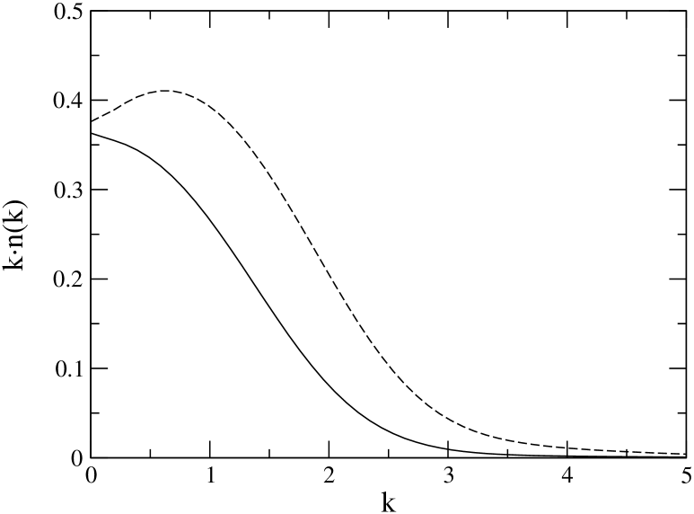
Figure 11: HS EL momentum distributions at $x=0.05$ (solid line) and $x=0.08$ (dashed line). Momenta in units of $a^{-1}$.

Fig. 11 shows the optimal momentum distribution at $x=0.08$ and 0.05. At the lowest $x$ values $k\,n(k)$ is a monotonically decreasing function of $k$. Actually, this is also the case in the Bogoliubov approximation at any density. When $x$ increases, $k\,n(k)$ develops a peak in the EL case at low $k$. This maximum can be considered as a genuine effect of the short range correlations in the EL approach. Notice that the value at the origin of $k\,n(k)$ results from a competition between $n_{0}$ and $c$. These two quantities largely vary with the density ($n_{0}$ decreases and $c$ increases with increasing density), but the overall variation of $\lim_{k\rightarrow 0}k\,n(k)$ is less pronounced.

V Dilute soft spheres

The soft spheres potential (Eq. (9)) is characterized by a core radius $R$ and a potential height $V_{0}$ that determine the scattering length $a$ according to Eq. (10). The SS scattering length is always smaller than the core radius, approaching it when $V_{0}$ increases. In the very dilute regime, HS and SS systems, having the same scattering length, are expected to have the same energy, while their separate kinetic and potential contributions may differ. Moreover, at low $x$–values the total energy is well reproduced by the two terms of the low density expansion of Eq. (1). In this section, we will study the deviations from this behavior and the influence of the shape of the potential on the energy and its components. To this aim, two SS potentials with the same scattering length and different radii are considered: the SS10 and SS5 potentials, having $R=10$ and $R=5$ in units of $a$, respectively. The corresponding heights are $V^{SS10}_{0}=0.00681670$ and $V_{0}^{SS5}=0.06308561$ in units of $\hbar^{2}/2ma^{2}$.

Table 3 reports the scaled total, kinetic and potential energies per particle for SS10 and SS5 in the EL, SR and UL cases, compared with the available exact DMC results boro99 at $x=0.0001$ and $x=0.01$. The low-density expansion yields ${\bar{E}}_{LD}/N(x=0.0001)=0.001317$ and ${\bar{E}}_{LD}/N(x=0.01)=0.1862$. The lower bound energies are ${\bar{E}}_{lb}(x=0.0001)=0.001257$ and ${\bar{E}}_{lb}(x=0.01)=0.1257$. The upper bound energies (31) depend on the shape of the potential, and, for SS10 and SS10, give: ${\bar{E}}_{ub}^{SS10}/N(x=0.0001)=0.0014277$, ${\bar{E}}_{ub}^{SS5}/N(x=0.0001)=0.0016516$, ${\bar{E}}_{ub}^{SS10}/N(x=0.01)=0.14277$, and ${\bar{E}}_{ub}^{SS5}/N(x=0.01)=0.16516$. Both, the upper and the lower bound properties are here satisfied. The shape dependence is weaker at low $x$, in fact the difference between the $SS10$ and $SS5$ energies is smaller at $x=0.0001$ than at $x=0.01$. On the other hand, the kinetic and potential energies exhibit a potential dependence at any $x$–value. The IPC results of Ref.sarsa02 are also given in the Table. The EL energies are very close to the DMC ones at $x=0.0001$ and the variational hiearchy is always fulfilled (DMC$<$EL$<$SR). As expected, the UL works better for the weaker SS10 potential, as well as the IPC wave function. The Jastrow wave function is variationally preferred to the IPC one at any $x$, as shown by the comparison between the EL and IPC energies. The good agreement between ${\bar{T}}_{g}$ and ${\bar{T}}_{n}$ seems to show that the HNC/0 approximation in the EL approach does not invalidate this conclusion.

The behavior of the scaled energy per particle along $x$ is shown in Fig. 12, in units of $4\pi x$, for the SS10, SS5 and HS potentials, in the EL, IPC and DMC cases, and compared with the upper bounds. The lower bound equals to unity in this units. Starting at $x\geq 10^{-3}$, clearly appears a shape dependence of the energy with the harder SS5 potential energies closer to the HS ones. Moreover, it is also to be stressed a dependence on the quality of the wave function in the same region, since differences between the Jastrow and IPC cases become evident for SS5. The quality of the upper bound improves when $R$ increases, because $V_{0}$ decreases at fixed $a$ and the perturbative expansion is expected to converge faster.

The energy and, in general, the structure of the ground state depends, to a large extent, on the two–body correlation factor employed. In the EL and UL cases, $f(r)$ is a derived quantity as the optimization is accomplished by varying $g(r)$ or $S(k)$. In the SR case, $f_{SR}(r)$ is an input function containing some variational parameters. In the present work for the SS gas we employ

$$f_{SR}(r)=1-be^{-cr^{2}}\ ,$$ (54)

which is flexible enough to obtain a reasonable value of the energy. Notice that the SS potential does not require the correlation function to be zero at the origin, so $b\neq 1$.

Figure 13 shows $g(r)$ for SS5 at $x=0.001$ in the EL, UL and SR cases and $f_{EL}^{2}(r)$. Many–body effects make $g_{EL}(r)$ quite different from $f_{EL}^{2}(r)$, both at low and intermediate $r$–values. The EL radial distribution function is softer at the origin, and, in general, less repulsive than the short-range one. The radial distribution function in the uniform limit approximation is close to $f_{EL}^{2}$ at small distances, approaching $g_{EL}(r)$ at $r\sim 5$. The radial distribution function obtained by the Bogoliubov approach (not shown in the figure) would exhibit, as for the HS case, an unphysically divergent behavior at short distances.

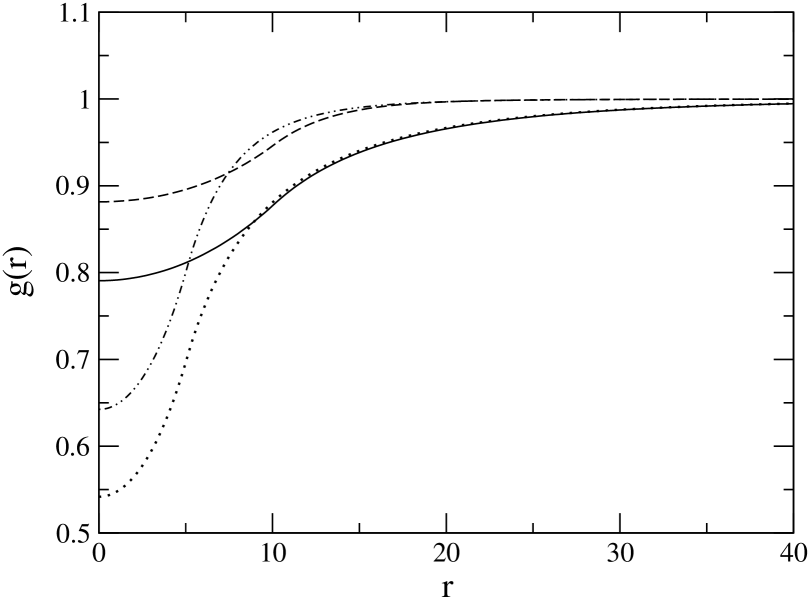
Figure 14: EL radial distribution functions for SS10 and SS5 at $x=0.0001$ (solid line for SS10 and dotted line for SS5) and $x=0.001$ (dashed line for SS10 and dashed–dot–dot line for SS5). Distances in units of $a$.

The dependence of the radial distribution function on the shape of the potential and on $x$ is illustrated in Fig. 14, containing the EL distribution functions for SS5 and SS10 at $x=10^{-4}$ and $x=10^{-3}$. The central hole of the radial distribution function is obviously deeper for the more repulsive SS5 potential. It becomes less pronounced at higher $x$, since the probability of finding two bosons at short relative distances increases with the density. The universal behavior in $x$ is recovered at large distances, where the Bogoliubov approach becomes reliable.

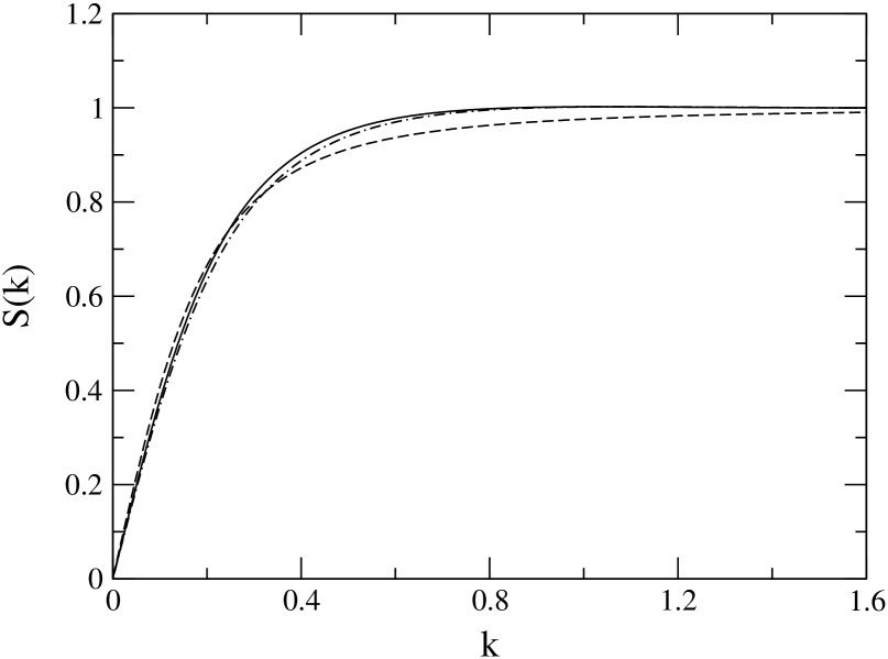
Figure 15: The SS static structure function $S(k)$ at $x=0.001$ for SS5. The solid, dashed and dot–dashed lines stand for the EL, Bogoliubov and the UL cases, respectively. Momenta in units of $a^{-1}$.

The static structure functions, in the EL, UL and Bogoliubov approaches, are plotted in Fig. 15 for the SS5 interaction. In all cases, $S(k)$ grows linearly at the origin, and the slope, governed by the sound velocity (Eq. (51)), is similar in all three cases. The Bogoliubov sound velocity, $c_{B}=\sqrt{16\pi x}$, is smaller than the UL estimate,

$$c_{UL}=\sqrt{\frac{8}{3}\pi R^{3}xV_{0}}\ ,$$ (55)

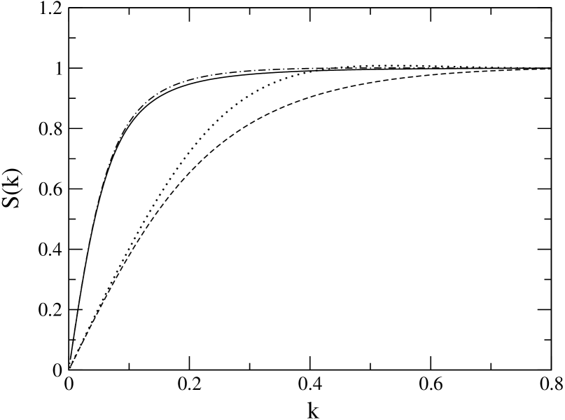
Figure 16: EL static structure functions for SS10 and SS5 at $x=0.0001$ ( solid line for SS5 and dot–dashed line for SS10), and $x=0.001$ (dashed line for SS5 and dotted line for SS10). Momenta in units of $a^{-1}$.

and consequently, the slope at low momenta in $S_{B}(k)$ is slightly larger than in $S_{UL}(k)$. $S_{UL}(k)$ approaches $S_{EL}(k)$ and the asymptotic value faster than $S_{B}(k)$. Actually, at a given density $S_{B}(k)$ and $c_{B}$ are identical for all the SS interactions with the same scattering length. The short-range $g(r)$ does not have the proper asymptotic behavior and produces a static structure function that does not vanish at the origin and does not increase linearly at low $k$. $S_{EL}(k)$ at $x=0.0001$ and $x=0.001$ are shown in Fig. 16 for SS5 and SS10. The SS10 sound velocity is smaller and the slope of $S(k)$ at the origin is larger. The differences are more evident at the largest $x$.

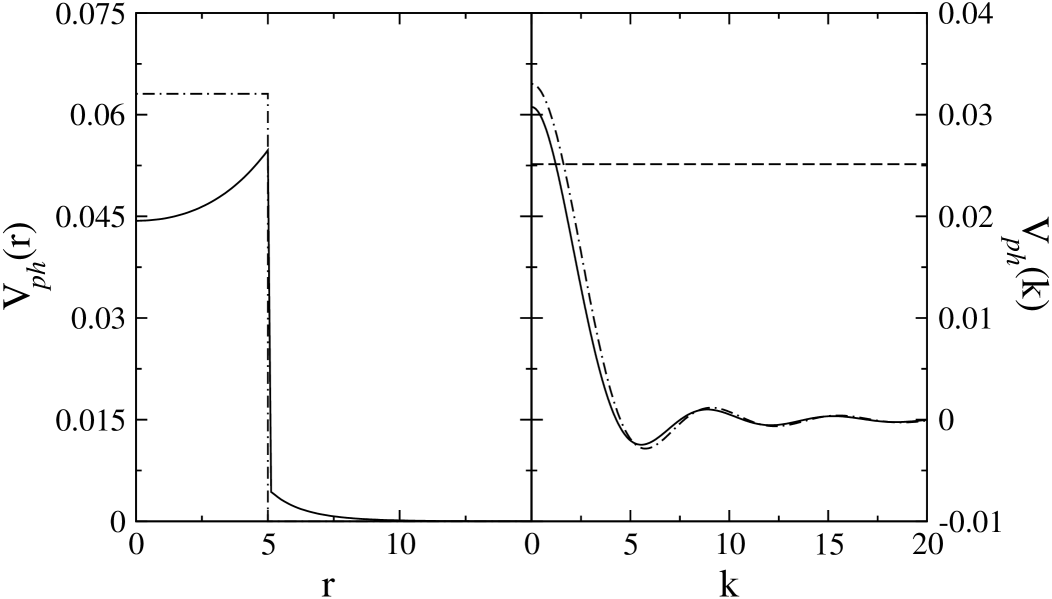
Figure 17: Particle-hole interaction in r–space (left panel) and in k–space (right panel), for SS5 at $x=0.001$. The solid and dot–dashed lines correspond to the El and UL cases, respectively. The dashed line in the right panel gives the Bogoliubov $V_{ph}$. Distances in units of $a$ and momenta in units of $a^{-1}$.

The particle-hole interaction corresponding to SS5 at $x=0.001$ is shown in Fig. 17 for the EL, UL and Bogoliubov approaches. The left and right panels give $V_{ph}(r)$ and its Fourier transform, $V_{ph}(k)$, respectively. $V_{ph}^{B}(r)=8\pi x\delta({\bf r})$ is not shown in the figure. The ph-interaction in the UL limit coincides with the interaction itself, $V_{ph}^{UL}(r)=V(r)$. $V_{ph}^{EL}(r)$ is discontinuous at $r=R$. The differences between $V_{ph}^{UL}(k)$ and $V_{ph}^{EL}(k)$ are larger at low momenta, consistently with the differences observed in the static structure function.

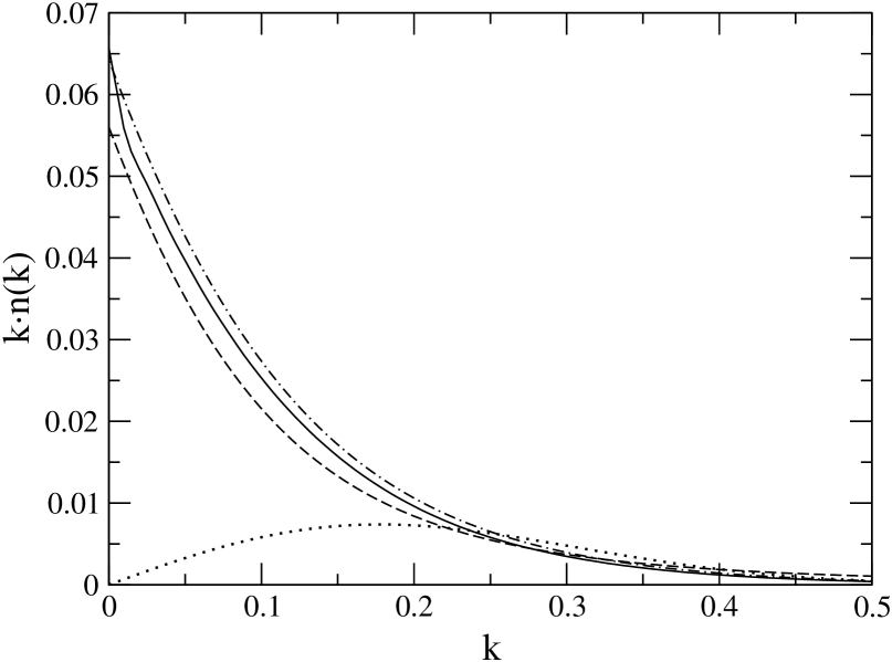
Figure 18: $k\,n(k)$ for SS5 at $x=0.001$. The solid, dashed, dash–dotted and dotted lines correpond to the EL, Bogoliubov, UL and SR results respectively. Momenta in units of $a^{-1}$.

Finally we discuss the results for the momentum distribution, $n(k)$. The quantity $k\,n(k)$ at $x=0.001$ is plotted in Fig. 18 for the SS5 interaction in the EL, Bogoliubov, UL and SR cases. All momentum distributions but the short-range one satisfy the long–wavelength behavior (53). Since $n_{SR}(k=0)\neq 0$, $k\,n_{SR}(k)=0$ at the origin. As in the HS case, $k\,n_{SR}(k)$ presents a maximum at intermediate momenta, as a byproduct of the absence of a long–range structure in the two–body correlation factor $f_{SR}(r)$.

In the $x$-range considered, $k\,n_{EL}(k)$ is a monotonously decreasing function of $k$. At higher $x$ it develops a maximum at low momenta, consistently with the HS results, also found in the high density homogenous atomic ⁴He. In the UL,

$$\lim_{k\rightarrow 0}{k\,n_{UL}(k)}=\frac{c_{UL}}{4}-\frac{k}{2}\,,$$ (56)

and the value at the origin depends on $x$ through the sound velocity, whereas its slope, $-1/2$, is independent on the density.

$k\,n_{B}(k)$ is also a decreasing function of $k$, its $k=0$ value being slightly smaller than the UL one, corresponding to a lower sound velocity. The UL momentum distribution for the SS potential decays as $k^{-8}$, and the condensate fraction can be computed by imposing the normalization condition. The condensate fractions and the kinetic energies obtained from the momentum distribution are reported in Table 3.

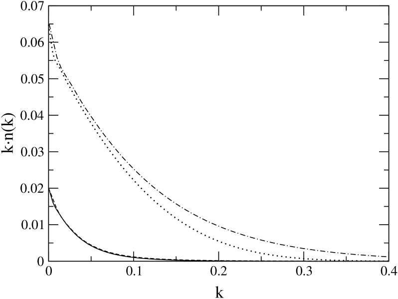
Figure 19: EL $k\,n(k)$ at $x=0.0001$ (solid line for SS10, dashed line for SS5) and $x=0.001$ (dotted line for SS10, dot–dashed line for SS5). Momenta in units of $a^{-1}$.

The dependence of $n(k)$ on the shape of the potential is studied in Fig. 19, where $k\,n_{EL}(k)$ is plotted at $x=0.0001$ and $x=0.001$ for SS5 and SS10. Apparently, the SS5 and the SS10 momentum distributions are identical at $x=0.0001$, pointing to a dependence only on the scattering length. This conclusion must be taken with caution, since in Table 3 more than a factor of two between the SS5 and SS10 kinetic energies, ${\bar{T}}_{n}$ , is found even at this low density.

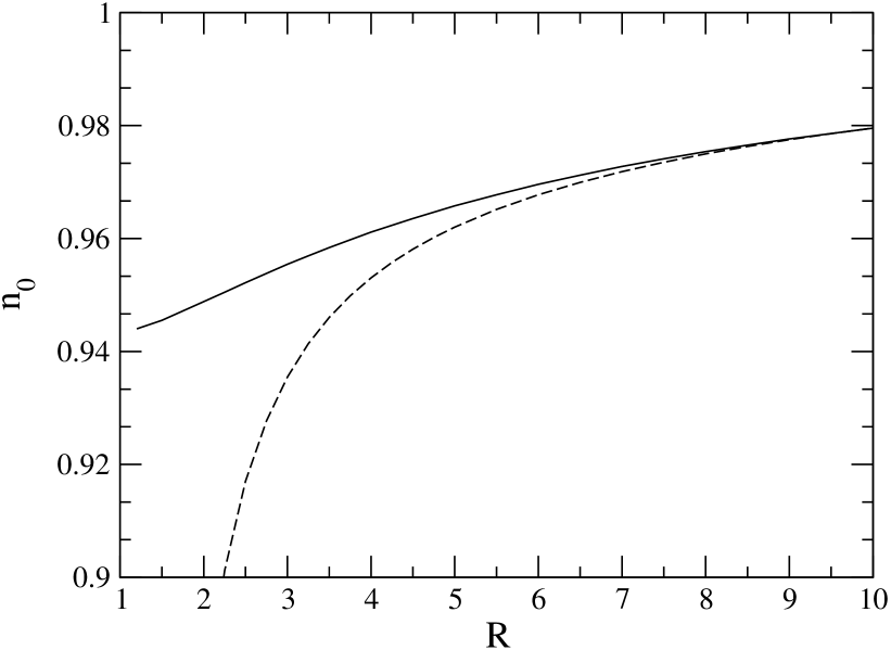
Figure 20: Condensate fraction for the soft sphere gas, at $x=0.001$, as a function of the radius, $R$, of the SS potential at fixed scattering length. EL, solid line; UL, dashed line. The Bogoliubov condensate fraction is $n_{0B}=0.952$. Distances in units of $a$.

The condensate fraction also depends on the shape of the potential. Figure 20 shows $n_{0,EL}$ and $n_{0,UL}$ at $x=0.001$ as a function of the radius of the SS potential, $R$, at a fixed value of the scattering length. As expected, the condensate fraction grows with $R$, since the interaction softens. The UL approach becomes accurate at large $R$–values, in the very weak interaction limit. In all cases, $n_{0,UL}$ is smaller than $n_{0,EL}$.

VI Summary and Conclusions

We have carefully investigated the energy and structure of a homogeneous gas of bosons interacting via hard and soft sphere potentials. We have adopted and compared several many-body approaches, as the variational correlated theory, the Bogoliubov model and the uniform limit approximation, valid in the weak interaction regime. When possible, the results have been compared with the exact diffusion Monte Carlo ones. A Jastrow type correlation appears to produce a good quality wave function if the hypernetted chain energy functional is freely minimized and the resulting Euler equation is solved. This is true for both hard and soft sphere interactions. The study of soft sphere potentials has confirmed the appearence of a shape dependence in the energy at $x\sim 0.001$, as already found by the IPC calculations of Ref.sarsa02 and by the DMC study of Ref.boro99 . We have numerically compared the EL results with those obtained in the uniform limit of weak interaction, in the Bogoliubov approximation and in the IPC theory. As expected, the differences are more relevant for the strongest interactions. The uniform-limit and independent-pair-correlation energies become more and more reliable as the interaction weakens. The universality breaks at much lower $x$–values for quantities different from the energy. For instance, the short range structure of the radial distribution functions (and, in consequence, the large momentum behavior of the static structure function) largely depends on the shape of the potential already at $x=0.0001$. We find a potential shape dependence in the SS condensate fraction at $x=0.001$. These results, as well as those for the energy, may help in evaluating the parameters entering the nonuniversal corrections in effective field theorybraaten01 , whose extraction from the available DMC calculations is heavily biased by the statistical errors.

The presence of a maximum in the correlated distribution function when $x$ increases has been discussed in details. The Bogoliubov model does not show this short range structure, independently on $x$. The excitation spectrum develops a rotonic maximum at large $x$, related to the shape of the particle–hole interaction. Again, the Bogoliubov approach, providing a constant $V_{ph}(k)$, does not allow for a roton–like excitation. The effect of the correlations is also apparent in the momentum distributions. In the hard sphere gas the CBF $kn(k)$ acquires a maximum at low momentum at $x\sim 0.06$. Both the Bogoliubov and the uniform limit (for soft spheres) approaches fail to reproduce this behavior.

The correlated basis functions theory may be extended to treat fermionic hard and soft spheres or mixtures of Fermi–Bose gases. Work along these lines is in progress. More challenging is the application of the CBF approach to trapped atomic gases, without resorting to local density type approximationsfabro99 . Employing the variational method in finite dilute systems presents mainly technical difficulties. However, it will probably represent the natural development of this technique.

$x$	${\bar{E}}_{DMC}/N$	${\bar{E}}_{EL}/N$	${\bar{E}}_{SR}/N$	$d$	${\bar{E}}_{LD}/N$
$10^{-6}$	$1.262\cdot 10^{-5}$	$1.264\cdot 10^{-5}$	$1.261\cdot 10^{-5}$	$480$	$1.260\cdot 10^{-6}$
$10^{-5}$	$1.274\cdot 10^{-4}$	$1.279\cdot 10^{-4}$	$1.277\cdot 10^{-4}$	$140$	$1.276\cdot 10^{-4}$
$10^{-4}$	$1.311\cdot 10^{-3}$	$1.316\cdot 10^{-3}$	$1.313\cdot 10^{-3}$	$90$	$1.317\cdot 10^{-3}$
$10^{-3}$	$1.424\cdot 10^{-2}$	$1.430\cdot 10^{-2}$	$1.428\cdot 10^{-2}$	$34$	$1.448\cdot 10^{-2}$
$5\cdot 10^{-3}$	$8.155\cdot 10^{-2}$	$8.206\cdot 10^{-2}$	$8.217\cdot 10^{-2}$	$15$	$8.422\cdot 10^{-2}$
$10^{-2}$	$1.796\cdot 10^{-1}$	$1.814\cdot 10^{-1}$	$1.819\cdot 10^{-1}$	$11$	$1.862\cdot 10^{-1}$
$5\cdot 10^{-2}$	$1.338$	$1.383$	$1.402$	$7$	$1.305$
$0.1$	$3.627$	$3.848$	$3.971$	$6$	$3.170$

Table 1: Scaled energy per particle for the hard spheres model, as a function of $x$. See text. $d$ is the healing distance corresponding to the correlation factor of Eq.(48), in units of the scattering length. In ${\bar{E}}_{LD}$ the first two terms of the expansion (1) have been used.

	$x$	${\bar{T}}_{g}/N$	${\bar{T}}_{n}/N$	$n_{0}$	$n_{0DMC}$	$n_{0B}$
EL	0.001	$1.430\cdot 10^{-2}$	$1.270\cdot 10^{-2}$	0.947	0.948	0.952
SR	0.001	$1.428\cdot 10^{-2}$	$1.290\cdot 10^{-2}$	0.940
EL	0.01	$1.814\cdot 10^{-1}$	$1.772\cdot 10^{-1}$	0.801	0.803	0.850
SR	0.01	$1.819\cdot 10^{-1}$	$1.975\cdot 10^{-1}$	0.799
EL	0.05	1.383	1.594	0.493	0.501	0.664
SR	0.05	1.402	1.543	0.481
EL	0.08	2.728	3.414	0.340		0.574
SR	0.08	2.794	3.451	0.327

Table 2: Scaled kinetic energy per particle of the HS gas calculated using the momentum distribution and the radial distribution function for the EL and SR wave functions at several values of $x$. $n_{0}$, $n_{0DMC}$ and $n_{0B}$ are the EL, DMC and Bogoliubov condensate fractions.

	$x$	$R$	${\bar{E}}/N$	${\bar{V}}/N$	${\bar{T}}_{g}/N$	${\bar{T}}_{n}/N$	$n_{0}$
EL	$10^{-4}$	10	$1.305\cdot 10^{-3}$	$1.202\cdot 10^{-3}$	$1.038\cdot 10^{-4}$	$1.000\cdot 10^{-4}$	0.988
SR	$10^{-4}$	10	$1.317\cdot 10^{-3}$	$1.241\cdot 10^{-3}$	$0.765\cdot 10^{-4}$	$0.765\cdot 10^{-4}$	0.997
UL	$10^{-4}$	10	$1.295\cdot 10^{-3}$	$1.184\cdot 10^{-4}$		$1.110\cdot 10^{-4}$	0.992
IPC	$10^{-4}$	10	$1.311\cdot 10^{-3}$
DMC	$10^{-4}$	10	$1.303\cdot 10^{-3}$				0.989
EL	$10^{-4}$	5	$1.314\cdot 10^{-3}$	$1.044\cdot 10^{-3}$	$2.708\cdot 10^{-4}$	$2.630\cdot 10^{-4}$	0.985
SR	$10^{-4}$	5	$1.361\cdot 10^{-3}$	$1.138\cdot 10^{-3}$	$2.231\cdot 10^{-4}$	$2.231\cdot 10^{-4}$	0.996
UL	$10^{-4}$	5	$1.231\cdot 10^{-3}$	$0.853\cdot 10^{-3}$		$3.780\cdot 10^{-4}$	0.982
IPC	$10^{-4}$	5	$1.331\cdot 10^{-3}$				0.987
DMC	$10^{-4}$	5	$1.309\cdot 10^{-3}$				0.989
EL	$10^{-2}$	10	$1.404\cdot 10^{-1}$	$1.394\cdot 10^{-1}$	$0.990\cdot 10^{-3}$	$0.981\cdot 10^{-3}$	0.980
SR	$10^{-2}$	10	$1.405\cdot 10^{-1}$	$1.395\cdot 10^{-1}$	$0.960\cdot 10^{-3}$	$0.960\cdot 10^{-3}$	0.977
UL	$10^{-2}$	10	$1.404\cdot 10^{-1}$	$1.395\cdot 10^{-1}$		$0.963\cdot 10^{-3}$	0.980
IPC	$10^{-2}$	10	$1.408\cdot 10^{-1}$
EL	$10^{-2}$	5	$1.532\cdot 10^{-1}$	$1.468\cdot 10^{-1}$	$6.445\cdot 10^{-3}$	$6.480\cdot 10^{-3}$	0.951
SR	$10^{-2}$	5	$1.535\cdot 10^{-1}$	$1.481\cdot 10^{-1}$	$5.350\cdot 10^{-3}$	$5.350\cdot 10^{-3}$	0.960
UL	$10^{-2}$	5	$1.528\cdot 10^{-1}$	$1.464\cdot 10^{-1}$		$6.375\cdot 10^{-3}$	0.950
IPC	$10^{-2}$	5	$1.556\cdot 10^{-1}$				0.953

Table 3: Scaled energies and condensate fractions for the soft sphere gas in the El, SR, UL, IPC and DMC approaches for two potentials having the same scattering length (see text) at $x=10^{-4}$ and $x=10^{-2}$.

Figure 12: Scaled energy per particle for the SS5 (triangles) and SS10 (circles) potentials in the EL (filled triangles and circles) and IPC (empty triangles and circles). The stars and crosses are the available DMC energies for SS10 and SS5, respectively. The solid line represents the EL energies for the HS potential. The horizontal lines give the upper bounds for the SS5 (dash–double dotted) and SS10 (dashed) potentials. In these units, the common lower bound equals 1.

Figure 13: Two-body distribution functions for the SS5 potential at $x=0.001$. The solid, dot–dashed and dashed lines correspond to the EL, UL and SR cases, respectively. The two–body correlation function, $f^{2}(r)$, as extracted from the EL $g(r)$ is plotted as a dotted line. Distances in units of $a$.