Non-exponential Dissipation in a Lossy Elastodynamic Billiard, Comparison with Porter-Thomas and Random Matrix Predictions

Abstract

We study the dissipation of diffuse ultrasonic energy in a reverberant body coupled to a waveguide, an analog for a mesoscopic electron in a quantum dot. A simple model predicts a Porter-Thomas like distribution of level widths and corresponding nonexponential dissipation, a behavior largely confirmed by measurements. For the case of fully open channels, however, measurements deviate from this model to a statistically significant degree. A random matrix supersymmetric calculation is found to accurately model the observed behaviors at all coupling strengths.

A random matrix model of wave scattering from an ideal lead, off a chaotic region, has been employed in nuclear theory for decades [1-6]. It originated in the theory of nuclear reactions and is widely used in the analysis of compound nuclei, mesoscopic quantum dots and microwave cavities [1-6]. It has provided a model of intrinsic loss mechanisms in classical wave chaotic systems, with implications for microwave cavities and reverberant ultrasonics. In particular it has been shown that dissipation is not necessarily exponential in time, and made specific predictions for how that decay should behave.

A simple argument that relates such behavior to the distribution of resonance widths leads to a non-exponential decay law under the assumption of a Porter-Thomas (chi-square) width distribution key-5 ; key-15 . That distribution follows from first order perturbation theory on a system with Gaussian mode shape statistics and a finite number of loss channels. A more general argument may be constructed by the information-theoretic approach key-2 or the random Hamiltonian approach key-4 ; key-8 . These also predict non-exponential decay and corresponding delay time distributions, but with different details key-4 ; key-5 ; key-11 . Acoustic key-15 and microwave key-14 measurements have confirmed non-exponential decays. Critical comparisons with the models have not been undertaken.

In this Letter we address diffuse energy decay in an open acoustical system. While non-exponential decays have long been observed, and modeled by means of Porter-Thomas distributions of resonance widths, deviations from those predictions have not yet been detected. Indeed, it has not yet been clear whether measurements can distinguish between the predictions of the simple argument and those of random matrix theory (RMT) [3–9]. It is therefore interesting to compare both the RMT predictions key-8 and the simple argument predictions key-15 with measurements conducted on an experimental realization of a chaotic billiard attached to a waveguide. In most cases we find that a Porter-Thomas model does an adequate job of fitting observed decay profiles. In the case of strongly coupled channels, however, a full RMT prediction is superior. The difference is small, but statistically significant.

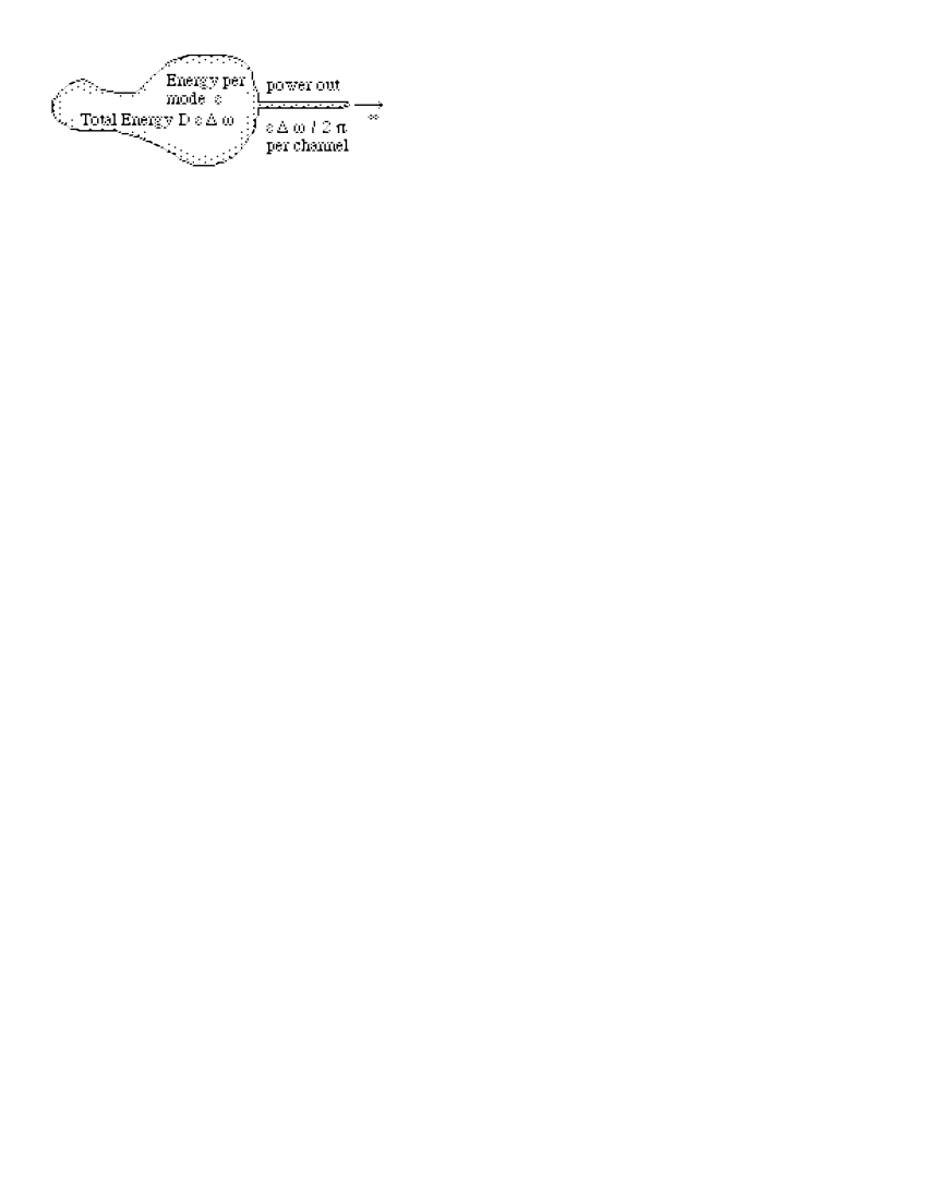
Figure 1: A diffuse wavefield radiates into a waveguide.

Consider a reverberant body as in Fig. 1 coupled to a waveguide. The body has mean diffuse energy density (per mode) of $\varepsilon$. The total energy in a band of width $\Delta\omega$ is $\varepsilon D\Delta\omega$, where the body’s modal density $D=\partial N_{Body}/\partial\omega$. An attached waveguide has mean energy per outgoing mode no greater than $\varepsilon$. Incoming modes have no energy. Each guided mode (i.e. each channel) therefore carries power at a rate no greater than $(d\Delta\omega)(\varepsilon/2)v_{g}$, where $d$ is the lineal modal density per length in the channel, $d=\partial N_{channel}/\partial\omega\partial L=1/\pi v_{g}$ and $v_{g}$ is the group velocity of that mode. The factor ($1/2$) is due to neglect of the incoming modes. Thus each channel conducts outgoing power $\Pi\leq(1/2\pi)\varepsilon\Delta\omega$, independent of dispersion in the channel. At maximal coupling each channel contributes the same mean partial width, an energy decay rate of $\Pi/\varepsilon D\Delta\omega=1/[2\pi\partial N_{Body}/\partial\omega]\equiv 1/t_{Heisenberg}$. This picture does not apply to individual normal modes of the body, but only to the mean. Those normal modes of the body which overlap well with the waveguide will dissipate rapidly; those which overlap poorly will do so slowly. While the average level width (and early time decay rate) may well correspond with the above estimate, the less strongly dissipated modes will eventually dominate a transient decaying field; the apparent dissipation rate will appear to diminish.

Modeling the diffuse field as a superposition of independent real normal modes with Gaussian statistics (this is not correct, lossy systems generically have complex eigenmodes), each with a proper decay rate given by first order perturbation theory, leads to a chisquare-like distribution of modal decay rates, and a net transient energy decay

$$E(t)=E_{0}\prod_{i=1}^{M}\left(1+2\sigma_{i}t\right)^{-1/2}$$ (1)

where $M$ is the number of open outgoing channels, and $\sigma_{i}$ is the decay rate through the $i$th channel, $\sigma_{i}\leq 1/t_{H}$. In certain limits, it reduces $E(t)\approx E_{0}\exp\left(-\sum_{i}\sigma_{i}t\right)$.

In the special case of equipotent channels, $\sigma_{i}=\sigma/M$, one recovers the simplest Porter-Thomas model key-15 ,

$$E(t)=E_{0}\left(1+2\sigma t/M\right)^{-M/2}$$ (2)

This form for the dissipation of ultrasonic energy density has been confirmed phenomenologically by taking $E_{0}$, $M$, and $\sigma$ to be adjustable parameters. Observed profiles $E(t)$ have been found to fit remarkably well key-15 . A particularly noteworthy case is that of key-14 in which the case of three weakly coupled ($\sigma_{i}\ll 1/t_{H}$) channels was successfully fit to Eq. (1). In many of these fits it has not been clear whether the recovered parameter $M$ is meaningful, i.e. whether it does indeed correspond to a discrete number of equipotent effective loss channels.

A better theory, beyond first order perturbation, is provided by considering a random matrix model key-3 ; key-4 for which level width distributions are known to be non-chisquare key-4 . Here the dynamics is governed by a (GOE) Gaussian random Hamiltonian, consistent with the assumed chaotic ray trajectories of the body, plus an anti-Hermitian part corresponding to a discrete number $M$ of outgoing channels. Supersymmetric techniques key-4 ; key-8 allow construction of various averages. Amongst the more easily constructed is $E(t)=\left|G_{ij}\left(t\right)\right|^{2}$, the mean square response at a site $j$ distinct from the site $i$ of the source, each distinct from any dissipative sites. $G_{ij}\left(t\right)$ is the time-domain Green’s function. On inverse Fourier transforming the result of a supersymmetric calculation key-8 one finds:

$$E(\tau)\sim\int_{1}^{\infty}\int_{1}^{\infty}d\lambda_{1}d\lambda_{2}\Pi\left(\tau,\lambda_{1},\lambda_{2}\right)f\left(\tau,\lambda_{1},\lambda_{2}\right)$$

$$\times\frac{\theta\left(\lambda_{1}\lambda_{2}-2\tau+1\right)\theta\left(2\tau-\lambda_{1}\lambda_{2}+1\right)\left(1-\left(2\tau+\lambda_{1}\lambda_{2}\right)^{2}\right)}{\left(\lambda_{1}^{2}+\lambda_{2}^{2}+\left(2\tau+\lambda_{1}\lambda_{2}\right)^{2}-2\lambda_{1}\lambda_{2}\left(2\tau+\lambda_{1}\lambda_{2}\right)-1\right)^{2}}$$ (3)

where, $\tau=t/t_{H}$, $M$ is the number of channels, each characterized by a coupling parameter $g_{i}\geq 1$, $f=\left(\lambda_{1}^{2}-1\right)\lambda_{2}^{2}+\left(\lambda_{2}^{2}-1\right)\lambda_{1}^{2}+1-\left(2\tau+\lambda_{1}\lambda_{2}\right)^{2}$, $\Pi=\prod_{i=1}^{M}\left(g_{i}+2\tau+\lambda_{1}\lambda_{2}\right)\left(g_{i}^{2}+2g_{i}\lambda_{1}\lambda_{2}+\lambda_{1}^{2}+\lambda_{2}^{2}-1\right)^{-1/2}$. For a large number of weak ($g_{i}\gg 1$) channels, this reduces to: $E(t)=E_{0}\exp\left(-\tau\sum 2/\left(g_{i}+1\right)\right)$, in agreement with the naive model. At finite $M$ the two models differ slightly. A comparison at $M=4$, $g_{i}=1.5$, $\sigma_{i}=2/\left(g_{i}+1\right)t_{H}=4/5t_{H}$ for all $i$, is shown in Fig. 2. The naive model overestimates curvature.

Figure 2: A comparison of the predictions of the Porter-Thomas model (dashed line, Eq. (1)) for transient decay with that of a full supersymmetric calculation (solid line, Eq. (3)).

We study the aluminum body (volume $561\,cm^{3}$, free surface $451\,cm^{2}$) pictured in Fig. 3. Non parallel faces and defocusing surfaces enhance ray-chaos. After preliminary baseline measurements, it was welded to an aluminum wire ($1100$ alloy, $3.18\,mm$ diameter, $3\,m$ length). Tests were carried out with the spiral part submerged in a water bath. Attenuation in the water assures negligible reflected energy and thus the presence of only outgoing waves. This was confirmed by separate measurements. The guided elastic waves of a circular waveguide are described by the Pochammer dispersion relation key-16 . All modes with azimuthal number $n>0$ are two-fold degenerate. At low frequency, below the first cutoff at $580\,kHz$, there are $M=4$ propagating guided waves. Two are flexural ($n=1$), one is extensional ($n=0$) and one torsional ($n=0$). A calculation of cutoff frequencies gives the number of open channels. The strength with which these channels are coupled is not known apriori. Measurement of reflections of waves incident from the wire onto the block indicate that the coupling is good; reflections are generally weak. Dispersion and the possibility of mode conversion complicate any attempt to be more quantitative.

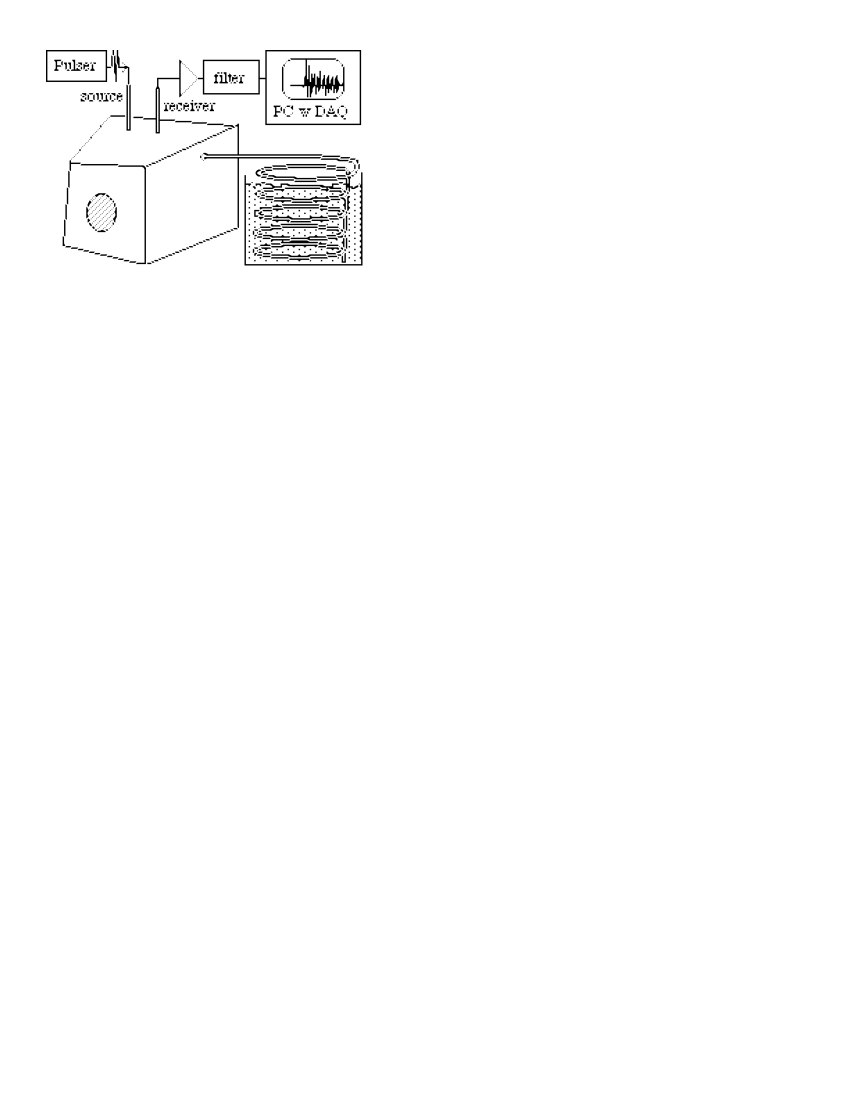
Figure 3: Sketch of measurement system.

Profiles $E(t)$ were constructed both before and after the waveguide was attached. For each case, piezoelectric pulses of negligible duration were applied to pin-transducers in light oil contact with the body, as in Fig. 3. Waveforms of durations of up to $100\,msec$, and bandwidths to $2\,MHz$ were recorded at a digitization rate of $5\,MSa/sec$. A low pass filter with a cutoff of $2.25\,MHz$ prevented aliasing. Repetition averaging improved signal to noise ratios and extended the system’s dynamic range. The resulting waveforms were time-windowed into $62$ successive $1.64\,msec$ sections with tapered edges. Each windowed waveform was Fourier transformed and squared and integrated over rectangular bins of width $25$ or $50\,kHz$. The result was an array of spectral energy densities versus time for each of several narrow frequency bands. On repeating this for $16$ distinct source and receiver positions an average $E(t)$ was constructed for each band. A typical profile is seen in Fig. 4. As expected, the waveguide has augmented the decay rate.

Figure 4: $\ln E(t)$ averaged over $16$ distinct positions of source and receiver in a band between $225$ to $275\,kHz$. The Heisenberg time is $34\,msec$.

The upper curve is the reference case without the waveguide; it shows a decay which is very nearly exponential, i.e. consistent with intrinsic decay mechanisms being widely distributed and corresponding to a large number of weakly coupled dissipative channels. As in key-15 , the behavior fits well to Eq. (2); chisquares are excellent. While the parameter M extracted from that fit is perhaps not meaningful, we do take Eq.(2) as a valid way to smooth the reference data. The smoothed reference $\ln E(t)$ is then subtracted from the measured $\ln E(t)$ in the waveguide-attached case to give a difference $\ln E$, what we would have measured in the attached case if our reference block had been non-dissipative. This profile shows substantial curvature, consistent with a hypothesis of a small number of outgoing channels.

The observed difference $\ln E$’s were then themselves fit to Eq. (2). Figs. 5 and 6 show the parameters $\sigma$ and $M$ extracted from those fits, and compares them with expectations based on assuming perfect coupling: $M_{Pochammer}=$ number of propagating modes; $\sigma=M_{Pochammer}/t_{H}$. That the $\sigma$ of the difference $\ln E$ is not in excess of this theory, even at high frequencies, is an indication that the welding process has not significantly increased intrinsic absorption. The correspondence is remarkably good for such a simple theory; $M$ and $\sigma$ show the predicted features, in particular those associated with the onsets of new guided modes at $580$, $800$ and $1000\,kHz$. At low frequencies, the correspondence is poor; the model assumption of perfect coupling is incorrect.

Figure 5: Decay rates $\sigma$ as recovered from a fit of the difference $\ln E(t)$’s to Eq. (2) in each of several narrow frequency bands (data points) are compared to the prediction: $\sigma=M_{Pochammer}/t_{H}$ (solid line).

Figure 6: $M$ values as recovered from fits to the difference $\ln E(t)$’s in each of several narrow frequency bands are compared to expectations based on the cutoff frequencies of the Pochammer dispersion relation.

The reduced chisquares of these fits are shown in the inset. At high frequencies they are within one standard deviation of the expected value of unity. Plots of the residuals show that fluctuations are not systematic. We conclude that the higher-frequency data is consistent with Eq. (2); small curvatures are well modeled by a single phenomenological parameter $M_{effective}$; the high frequency data does not permit conclusions in regard to the relative virtues of the various theories. At low frequency the chisquares exceed unity. This is in part due to the inadequacy of our spatial averaging there; different transducer positions are often within a wavelength and are correlated. It is in part also due to some systematic deviations that indicate a need for a better theory; unphysical values of $M$ (Fig. 6) are a further indication of that need.

Figure 7: Values for $t_{H}\sum\sigma_{i}$ (dashed line) and for $\sum 2/\left(1+g_{i}\right)$ (solid line) from fits of Eq. (1) and Eq. (3) to the difference $\ln E(t)$ profiles. The chisquares of the fits indicate Eq. (1)’s inability to fit the data in those places where coupling is strong.

Figure 8: Fits of the supersymmetric profile (Eq. (3)) (smooth solid lines) and the Porter-Thomas model (Eq. (1)) (dashed lines) to the difference $\ln E(t)$’s (irregular solid lines) in representative frequency bins. At $150\,kHz$ each model fits well: Eq. (1) calls for $\sigma_{i}=\left\{1,\,1,\,0.07686,\,0.07686\right\}/t_{H}$ (the flexural modes are especially weakly coupled at such long wavelength, hence their small $\sigma$’s.) Eq. (3) calls for $2/\left(1+g_{i}\right)=\left\{0.5954,\,1,\,0.0614,\,0.0614\right\}$. At $475\,kHz$, the fits call for $\sigma_{i}=1/t_{H}$ and $2/\left(1+g_{i}\right)=0.9$ for all $i$,

At low frequencies ($<580\,kHz$), where there are only four open channels, we attempt a fit to the richer theories ($1$) and ($3$) by fixing $M$ at four and adjusting the coupling strengths. We take the two flexural waves to have identical coupling (the weld is axisymmetric); set $g_{3}=g_{4}$, $\sigma_{3}=\sigma_{4}$, and adjust only $E_{0}$ and three values of $g_{i}\geq 1$ (or $\sigma_{i}\leq 1/t_{H}$). The fits’ values for total loss coefficient ($t_{H}\sum\sigma_{i}\leq 4$ and $\sum 2/\left(1+g_{i}\right)\leq 4$) are shown in Fig. 7. Representative plots of the data and fits are shown in Fig. 8. In cases with weak coupling, both models do well. At higher frequencies where coupling is efficient (all $g$’s close to unity), and first order perturbation theory is invalid, there are significant discrepancies. At several of the frequencies only the full RMT calculation Eq. (3) is statistically acceptable. At a few other frequencies where Eq. (1) gives an acceptably low chisquare, its call for all four channels to be perfectly coupled, $\sigma_{i}=1/t_{H}$, is implausible. The fits at these several frequencies may be the first demonstration of non-Porter-Thomas like level width distributions; it is also evidence for the superior applicability of a full RMT calculation over that of simpler theories. This has implications for RMT and wave chaos, for mesoscopics, nuclear physics, microwave physics, diffuse field ultrasonics, and also for structural acoustics where modeling of losses, both intrinsic and radiative key-17 ; key-18 , is gathering increased attention.

This work was supported by NSF grant CMS-0201346.

References

- (1) C. Mahaux, H.A. Weidenmüller, Shell-Model Approach to Nuclear Reactions. (North-Holland, Amsterdam, 1969).
- (2) P.A. Mello, H.U. Baranger, Waves in Random Media 9, 105 (1999); C. W. J. Beenakker, Rev. Mod. Phys. 69, 731 (1997)
- (3) T. Guhr, A. Müller-Groeling, H.A. Weidenmüller, Phys. Rep. 299, 189 (1998); H.-J. Stöckmann. Quantum chaos. An Introduction. (Cambridge University Press, 1999); Y. Alhassid, Rev. Mod. Phys. 72, 895 (2000).
- (4) Yan V. Fyodorov, H.-J. Sommers, J. Math. Phys. 38, 1918 (1997).
- (5) J. M. Verbaarschot, H.A. Weidenmüller and M.R. Zirnbauer, Phys. Rep. 129, 367 (1985); J. M. Verbaarschot, Ann. of Physics, 168, 138 (1986); K. Efetov. Supersymmetry in disorder and chaos (Cambridge University Press, 1997).
- (6) F.-M. Dittes, Phys. Rep. 339, 215 (2000).
- (7) J. Burkhardt, R. L.Weaver, Journal of Sound and Vibration 196, 147 (1996); J. Burkhardt, Ultrasonics 36, 471 (1986); O.I. Lobkis, R.L. Weaver, I. Rozhkov, Journal of Sound and Vibration 237, 281 (2000); M R Schroeder, 5th Int. Congress of Acoustics p G31 (1965).
- (8) D. V. Savin, V. V. Sokolov, Phys. Rev. E 56 (1997); H.-J. Sommers, D. V. Savin, V. V. Sokolov, Phys. Rev. Lett. 87, 094101 (2001); D. V. Savin, H.-J. Sommers, cond-mat/0303083 v2 (2003); P. W. Brouwer, K. M. Frahm, and C. W. J. Beenakker, Phys. Rev. Lett. 78, 4737 (1997); Waves Random Media 9, 91 (1999); M.G.A. Crawford, P.W. Brouwer, Phys. Rev E 65, 026221 (2002).
- (9) H. Alt, H.-D. Gräff et al, Phys. Rev. Lett. 74, 62, (1995).
- (10) K. F. Graff, Wave Motion in Elastic Solids, Dover, NY 1975.
- (11) R. L. Weaver, J. Acoust. Soc. Am. 101, 1441-49 (1997).
- (12) A. D. Pierce, V. Sparrow and K. Russell, J. Vib. Acoust. 117 339-348 (1995).