Magnetotransport in two-dimensional electron gas at large filling factors

Abstract

We derive the quantum Boltzmann equation for the two-dimensional electron gas in a magnetic field such that the filling factor $\nu\gg 1$. This equation describes all of the effects of the external fields on the impurity collision integral including Shubnikov-de Haas oscillations, smooth part of the magnetoresistance, and non-linear transport. Furthermore, we obtain quantitative results for the effect of the external microwave radiation on the linear and non-linear $dc$ transport in the system. Our findings are relevant for the description of the oscillating resistivity discovered by Zudov et al., zero-resistance state discovered by Mani et al. and Zudov et al., and for the microscopic justification of the model of Andreev et al.. We also present semiclassical picture for the qualitative consideration of the effects of the applied field on the collision integral.

I Introduction

The purpose of this paper is to construct the theory describing linear magnetotransport, non-linear effect of $dc$ electric field, and effect of microwave on both linear and nonlinear $dc$ magnetotransport from a unified point of view. Despite a long history of the systematic experimental and theoretical study of the properties of two-dimensional electron and hole systems in semiclassically strongAndoreview and quantizing magnetic fieldQHEreview , the system still brings us surprises.

Recent experiments Zudov1 ; Mani ; Zudov2 ; Mani2 ; Dorozhkin ; Zudov4 revealed the new class of phenomena. (In fact, such effects were first considered theoretically by RyzhiiRyzhii ; Ryzhii1 three decades ago but were not fully appreciated.) Exposing the two-dimensional electron system to a microwave radiation, Zudov et al.Zudov1 discovered the drastic oscillations of the longitudinal resistivity as a function of the magnetic field. The period of these oscillations was controlled only by the ratio of the microwave frequency $\omega$ to the cyclotron frequency $\omega_{c}$. Moreover, the oscillations were observed at relatively high temperature, $T$, such that usual Shubnikov-de Haas oscillations in the absence of the microwave irradiation were not seen, $T\gtrsim\hbar\omega_{c}$. Working with cleaner samples, almost simultaneously, two experimental groups Mani ; Zudov2 reported observations of a novel zero-resistance state in two-dimensional electron systems, appearing when the oscillations of the resistivity hit zero. It is worth emphasizing that the zero-resistance state was not connected to any significant features in the Hall resistivity in contrast to that for the Quantum Hall EffectQHEreview . Further experimental activity consisted in analysis of the low-field part of the oscillations in order to understand the effect of the spin-orbit interactionMani2 and observation of the zero-conductance state in the Corbino disk geometryZudov4 . Results Mani ; Zudov2 were later confirmed by an independent experiment.Dorozhkin

Two recent theoretical papersDurst ; Andreev are likely to explain the main qualitative features of the dataZudov1 ; Mani ; Zudov2 ; Mani2 ; Dorozhkin ; Zudov4 . Durst et al.Durst presented a physical picture and a calculation of the effect of microwave radiation on the impurity scattering processes of a two dimensional electron gas [see also Ref. Ryzhii1, ]. In addition to obtaining big oscillations of the magnetoresistance with the right period of Ref. Zudov1, . the crucial result of Refs. Ryzhii, ; Ryzhii1, ; Durst, is the existence of the regimes of magnetic field and applied microwave power for which the longitudinal linear response conductivity is negative,

$$\sigma_{xx}<0.$$ (1)

It was shown by Andreev et al.Andreev that Eq. (1) by itself suffices to explain the zero-$dc$-resistance state observed in Refs. Mani, ; Zudov2, , independent of the details of the microscopic mechanism which gives rise to Eq. (1). The essence of Andreev et al.Andreev result is that a negative linear response conductance implies that the zero current state is intrinsically unstable: the system spontaneously develops a non-vanishing local current density, which almost everywhere has a specific magnitude $j_{0}$ determined by the condition that the component of electric field parallel to the local current vanishes, see also Sec. VII of the present paper. The existence of this instability was shown to be the origin of the observed zero resistance state. It is worth mentioning that the instability of the systemGunn with absolute negative conductivity is known since the work of Zakharov.Zakharov The important new feature of the instability and the domain structure of Andreev et al. Andreev , that the instability occurs at large Hall angle; as the result the domains for the current coincide with the domains of the electric field directed perpendicular to the current. We also would like to notice the certain similarity with the model of photoinduced domains proposed by D’yakonovDyakonov as an explanation of the experiments on ruby crystals under the intense laser irradiationRuby .

Subsequent theoretical works outlined ideasAnderson ; HeandShe ; Volkov of Ref. Durst, ; Andreev, ; postulatedMikhailov the plasma drift instability; considered “a simple classical model for the negative dc conductivity” due to non-parabolicity of the spectrum newRaikh or due to the lattice effects on ac-driven 2D electrons.Rivera We will not discuss those works further in a present paper.

Unfortunately, the comprehensive quantitative description of the dataZudov1 ; Mani ; Zudov2 is not possible within Refs. Durst, ; Ryzhii, ; Ryzhii1, . Moreover, phenomenology of Refs. Andreev, implies certain form of the non-linear $dc$ transport in the presence of the microwave radiation which has not been microscopically justified yet. Our article presents a program for such a description. However, we will not take into account effects which depend on the distribution function and are determined by inelastic processes, see Ref. Mirlin-ac and Section II.1. These effects will be considered elsewhere.inelastic

The paper is organized as follows. Qualitative discussion based on a consideration of semiclassical periodic orbits is presented in Sec. II. The quantum Boltzmann equation applicable for large filling factors and small angle scattering on the impurity potential is derived in Sec. III. This equation is later used to obtain closed analytic formulas for linear-$dc$ transport, Sec. IV, non-linear $dc$ transport, Sec. V, and the effect of microwave radiation on the $dc$ transport, Sec. VI. Section VII relates the results to the model of domains of Ref. Andreev, . Our findings are summarized in Conclusions.

II Qualitative discussion

The qualitative discussion of the effect of the microwave radiation on the $dc$-transport was presented in Refs. Ryzhii, ; Ryzhii1, ; Durst, in terms of quantum transitions between Landau levels. We chose to utilize the fact that only electrons with large Landau level indices are important and explain the effects in terms of semiclassical periodic motion. This explanation becomes especially convenient when the Landau levels are significantly broadened, which means that the number of the repetitions in the periodic orbit is small. [Infinite number of the repetitions of the periodic orbit would correspond to the vanishing width of the Landau levels.] Moreover, the qualitative picture will enable us to separate effects into two groups according to their sensitivity to the electron distribution function, and understand the status and validity of the approximation which will be made in the technical part of the paper.

To analyze the effect of external fields on the collision processes, it is more convenient to switch into the moving coordinate frame

$$\mbox{\boldmath$r$}\to\mbox{\boldmath$r$}-\mbox{\boldmath$\zeta$}(t),$$ (2)

in which the external electric field is absent. The position of the moving frame $\mbox{\boldmath$\zeta$}(t)$ is found from

$$\partial_{t}\mbox{\boldmath$\zeta$}(t)=\left(\frac{\partial_{t}-\omega_{c}\hat{\varepsilon}}{\partial_{t}^{2}+\omega_{c}^{2}}\right)\frac{e\mbox{\boldmath$E$}(t)}{m_{e}},$$ (3)

where $\mbox{\boldmath$E$}(t)$ is the applied spatially homogeneous electric field, $m_{e}$ is the electron band mass, $\omega_{c}=\frac{eB}{m_{e}c}$ is the cyclotron frequency, and $\hat{\varepsilon}$ is the antisymmetric tensor: $\varepsilon_{xy}=-\varepsilon_{yx}=1,\varepsilon_{xx}=\varepsilon_{yy}=0$.

If there were no disorder potential, the distribution function $f(\varepsilon)$ of the electrons in this moving frame would be the Fermi function

$$f(\varepsilon)=f_{F}(\varepsilon)=\frac{1}{1+e^{\varepsilon/T}},$$ (4)

no excitations would appear and therefore no dissipative current would be possible. On the classical level, an electron experiences the cyclotron motion with the position of the guiding center $R$ intact. Collision with impurities moving with velocity $\partial_{t}\mbox{\boldmath$\zeta$}$ cause the drift of the guiding center, so that the current density

$$\mbox{\boldmath$j$}^{(d)}=eN_{e}\left(\frac{d\mbox{\boldmath$R$}}{dt}\right)_{coll}$$ (5)

arises. Here, $N_{e}$ is the electron density, and $\left(d\mbox{\boldmath$R$}/dt\right)_{coll}$ symbolizes the probabilistic change in the position of the guiding center to be discussed below.

Let us consider the scattering process of the electron off one impurity. Because the size of the scattering region (correlation length of the potential $\xi$) is much smaller than the cyclotron radius, we can still characterize the scattering process by the initial direction $i$, and the scattering angle $\theta$ as shown on Fig. 1. We consider only small angle scattering

$$\theta\ll 1.$$ (6)

In this case, each scattering event causes the shift in the position of the guiding center

$$\Delta\mbox{\boldmath$R$}=-\mbox{\boldmath$i$}R_{c}\theta,$$ (7)

where $R_{c}=v_{F}/\omega_{c}$ is the cyclotron radius and $v_{F}$ is the Fermi velocity, see Fig. 1.

During the collision process impurity moves with the velocity $-\partial_{t}\mbox{\boldmath$\zeta$}(t)$. Because the size of the impurity is small, and we assume that $|\partial_{t}\mbox{\boldmath$\zeta$}(t)|\ll v_{F}$, this motion can be neglected in the calculation of the scattering amplitude but it has to be taken into account in the conservation of energy. Indeed, during the scattering event the moving impurity transfers the energy $\Delta\varepsilon=-\partial_{t}\mbox{\boldmath$\zeta$}(t)\cdot\Delta{\mbox{\boldmath$p$}}$, where change of the electron momentum is given by

$$\Delta\mbox{\boldmath$p$}=-\hat{\varepsilon}\mbox{\boldmath$i$}p_{F}\theta$$ (8)

for $\theta\ll 1$, and $p_{F}=m_{e}v_{F}$ is the Fermi momentum.

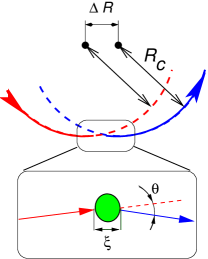
Figure 1: Scattering process off a single impurity. Inset shows the semiclassical trajectory in the vicinity of the impurity.

Taking this energy change into account we write for the displacement of the center of orbit

$$\begin{split}&\frac{1}{R_{c}}\left(\frac{d\mbox{\boldmath$R$}}{dt}\right)_{coll}\\ &=\Big{\langle}\int d\theta\frac{\Delta\mbox{\boldmath$R$}}{R_{c}}\int d\varepsilon\left\{f\left(\varepsilon\right)-f\left(\varepsilon+\Delta\varepsilon\right)\right\}{\cal M}\Big{\rangle}_{\mbox{\boldmath$i$}}\\ &=\Big{\langle}\mbox{\boldmath$i$}\int d\theta\,\theta\int d\varepsilon\frac{\partial f(\varepsilon)}{\partial\varepsilon}\left(\partial_{t}\mbox{\boldmath$\zeta$}(t)\cdot\Delta{\mbox{\boldmath$p$}}\right){\cal M}\Big{\rangle}_{\mbox{\boldmath$i$}},\end{split}$$ (9)

where the function ${\cal M}(\theta)$ is proportional to the scattering cross-section and is determined by the impurity potential. We will assume that ${\cal M}(\theta)$ vanishes rapidly at $\theta\sim\hbar/(p_{F}\xi)\ll 1$, i.e. Eq. (6) holds. In Eq. (9), $\langle\dots\rangle_{\mbox{\boldmath$i$}}$ stands for the averaging over the direction of the momentum of the electron incoming on the impurity.

Substituting Eq. (8) into Eq. (9), one finds

$$\left(\frac{d\mbox{\boldmath$R$}}{dt}\right)_{coll}=-\left(\frac{R_{c}}{\tau_{tr}}\right)\left(\frac{\hat{\varepsilon}\partial_{t}\mbox{\boldmath$\zeta$}}{v_{F}}\right),$$ (10)

where

$$\frac{1}{\tau_{tr}}=\frac{p_{F}v_{F}}{2}\int d\theta\theta^{2}{\cal M}(\theta)$$ (11)

is the transport scattering time at zero magnetic field. Together with Eq. (5) this gives the Drude formula $\sigma_{xx}=\frac{e^{2}N_{e}}{m\omega_{c}^{2}\tau_{tr}}$ for the large Hall angle $\omega_{c}\tau_{tr}\gg 1$.

It is not the end of the story though. Considering one scattering event as a complete real process, we imply that there are no returns of an electron to the same impurity, or, to be more precise, the possible returns are not correlated with original scattering. However, in magnetic field an electron moves along a circle of the cyclotron radius $R_{c}$ between shattering processes. This circular motion results in correlated returns of the electron to the same impurity. [To the best of our knowledge the first discussion of the magnetoresistance in terms of returning semiclassical orbits was performed in Ref. Baskin79, ]

Such returns do not change the structure of Eq. (9), but they do change the scattering cross-section ${\cal M}(\theta)$ in comparison with its value in zero magnetic field. Indeed, one can see from Fig. 2 that several semiclassical paths characterized by different number of rotations and different instances of the impurity scattering contribute to the same final state; amplitudes for such processes $A_{l}^{\alpha}(\theta)$ sum up coherently.

$$\begin{split}{\cal M}(\theta)&\propto\left|\sum_{l,\alpha}{A_{l}^{\alpha}(\theta)}\right|^{2}\\ &=\left|{A_{0}(\theta)}\right|^{2}+2\mbox{$\mathrm{R}e$}\sum_{l,l^{\prime},\ \alpha\neq\alpha^{\prime}}{A_{l^{\prime}}^{\alpha^{\prime}}(\theta)}\left[A_{l}^{\alpha}(\theta)\right]^{*},\end{split}$$ (12)

where index $l$ labels the number of rotation and $\alpha$ labels semiclassical paths; Fig. 2 shows the paths for $l=1,2$, while Fig. 1 depicts the path for $l=0$. Equation (9) takes into account the contribution from the shortest trajectory (first term in the second line) of Eq. (12) and misses the interference contributions.

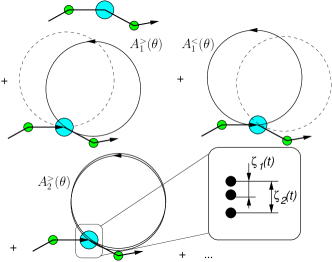
Figure 2: Different amplitude giving coherent contributions into the impurity scattering cross-sections. Inset shows the shift of the impurity between the scattering events in moving coordinate frame.

To assess the role of the interference contributions, let us employ the Born approximation of the impurity scattering. Then, each semiclassical path may involve only one scattering off an impurity, and all the paths are classified by (i) the scattering angle $\theta$ and (ii) whether the impurity affects the electron in the beginning or in the end of the path; we will call corresponding amplitudes $A^{>}_{l}(\theta)$ and $A^{<}_{l}(\theta)$, see Fig. 2. Factorizing the impurity scattering potential into the scattering cross-section at zero magnetic field ${\cal M}_{0}(\theta)$, we obtain

$${\cal M(\theta)}={\cal M}_{0}(\theta)\left\{1+2\mbox{$\mathrm{R}e$}\sum_{l,l^{\prime}}{A_{l^{\prime}}^{>}(\theta)}\left[A_{l}^{<}(\theta)\right]^{*}\right\}.$$ (13)

Equation (13) neglects the motion of the impurity during the whole collision process. Apparently, it is consistent with the derivation of Eq. (9) where the effect of the impurity motion on the matrix elements was also neglected. Indeed, for the process in Fig. 1, $l=0$, the characteristic scattering time can be estimated as $\Delta t=\xi/v_{F}$. The displacement of the impurity is, then, $|\Delta\mbox{\boldmath$r$}|=|\partial_{t}\mbox{\boldmath$\zeta$}|\cdot(\xi/v_{F})\ll\xi$, for $|\partial_{t}\mbox{\boldmath$\zeta$}|\ll v_{F}$, and could be neglected. However, for the scattering shown in Fig. 2 the interfering processes are separated in time by the interval $\Delta t=\frac{2\pi l}{\omega_{c}}$. Displacement during such interval is $\Delta|\mbox{\boldmath$r$}|\simeq|\partial_{t}\mbox{\boldmath$\zeta$}|\cdot\left(\frac{2\pi l}{\omega_{c}}\right)=|\partial_{t}\mbox{\boldmath$\zeta$}|\left(\frac{\xi}{v_{F}}\right)\left(\frac{2\pi lR_{c}}{\xi}\right)$. Because $R_{c}\gg\xi$, the displacement may easily become comparable with the impurity size $\xi$ even for $|\partial_{t}\mbox{\boldmath$\zeta$}|\ll v_{F}$. Therefore the displacement must be taken into account in the interference terms in Eq. (13). Due to the impurity motion, the scattering off impurity occurs at different points, see inset in Fig. 2. In this respect, the scattering off a moving impurity is analogues to the interference in a grate interferometer with the distance between slits equal to $\mbox{\boldmath$\zeta$}_{l}(t)=\mbox{\boldmath$\zeta$}\left(t-\frac{2\pi l}{\omega_{c}}\right)-\mbox{\boldmath$\zeta$}\left(t\right)$. By analogy with the grate interferometer, we find that Eq. (13) has to be modified as

$${\cal M}={\cal M}_{0}(\theta)\left\{1+2\mbox{$\mathrm{R}e$}\sum_{l,l^{\prime}}{A_{l^{\prime}}^{>}}\left[A_{l}^{<}\right]^{*}\exp\left[\frac{i\Delta\mbox{\boldmath$p$}\cdot\mbox{\boldmath$\zeta$}_{l}\left(t\right)}{\hbar}\right]\right\},$$ (14)

where $\Delta\mbox{\boldmath$p$}$ is given by Eq. (8). Finally, the quantum mechanical amplitudes $A_{l}^{>,<}(\theta)$ can be decomposed into the smooth prefactor $a$ and the rapidly oscillating exponent involving the reduced action along a semiclassical cyclotron trajectory

$$A_{l}^{>,<}=a_{l}^{>,<}\exp\left[il\left(\frac{\pi p_{F}^{2}\lambda_{H}^{2}}{\hbar^{2}}+\frac{2\pi\varepsilon}{\hbar\omega_{c}}\right)\right],$$ (15)

with $\lambda_{H}=\left(\frac{\hbar c}{eB}\right)^{1/2}$ being the magnetic length.

Having investigated the effect of the returning paths on the scattering process, we are ready to write an expression for the dissipative current. Substituting Eqs. (14) and (15) into Eq. (9), we find

$$\begin{split}\left(\frac{d\mbox{\boldmath$R$}}{dt}\right)_{coll}&=R_{c}\Bigg{\langle}\mbox{\boldmath$i$}\int d\theta\,\theta{\cal M}_{0}(\theta)\int d\varepsilon\frac{\partial f(\varepsilon)}{\partial\varepsilon}\left(\partial_{t}\mbox{\boldmath$\zeta$}(t)\cdot\Delta{\mbox{\boldmath$p$}}\right)\\ &\times\left\{1+2\mbox{$\mathrm{R}e$}\sum_{l,l^{\prime}}{a_{l^{\prime}}^{>}}\left[a_{l}^{<}\right]^{*}\exp\left(\frac{i\Delta\mbox{\boldmath$p$}\cdot\mbox{\boldmath$\zeta$}_{l}\left(t\right)}{\hbar}+\frac{i\pi(l^{\prime}-l)p_{F}^{2}\lambda_{H}^{2}}{\hbar^{2}}+\frac{i\pi(l^{\prime}-l)\varepsilon}{\hbar\omega_{c}}\right)\right\}\Bigg{\rangle}_{\mbox{\boldmath$i$}},\end{split}$$ (16)

Equation (16) is the main qualitative result of this section . It shows, that due to the presence of the returning orbits on one hand, and the largeness of the period on the other hand, the scattering process is extremely sensitive to external fields applied to the system. As the result, a rich variety of the effects arises. The effects can be separated into two groups: (i) sensitive to the distribution function; and (ii) non-sensitive to the electron distribution. We will discuss those groups separately in following two subsections.

II.1 Effects dependent on the form of distribution function

Retaining only the contributions from the amplitudes with different winding numbers in Eq. (16), and considering only linear terms in $\zeta$, we obtain familiar Shubnikov – de Haas oscillations $\rho_{osc}$ of the resistivity $\rho_{xx}(B)$:

$$\frac{\rho_{osc}(B,T)}{\rho_{xx}(B=0)}=\sum_{m=1}\eta_{m}\Upsilon_{m}\cos\left(\frac{\pi mp_{F}^{2}\lambda_{H}^{2}}{\hbar^{2}}\right)$$ (17)

where

$$\Upsilon_{m}=-\int d\varepsilon\frac{\partial f(\varepsilon)}{\partial\varepsilon}\exp\left[\frac{i2\pi m\varepsilon}{\hbar\omega_{c}}\right]$$ (18)

The form-factors, $\eta_{m}\simeq\sum_{l}a_{l}^{<}[a_{l+m}^{>}]^{*}$ are determined by the impurities at which scattering may occur during the circular motion of the electron, see Sec. II.3 for a more detailed discussion. The accurate expression for the factors $\eta_{m}$ are written in Sec. IV.2.

Neglecting the effect of the applied electric field on the electron distribution function $f(\varepsilon)$, i.e. $f(\varepsilon)=f_{F}(\varepsilon)$ see Eq. (4), we obtain

$$\Upsilon_{m}=\frac{2\pi^{2}mT}{\hbar\omega_{c}\sinh\left(\frac{2\pi^{2}mT}{\hbar\omega_{c}}\right)}.$$ (19)

Therefore, the Shubnikov – de Haas oscillations are exponentially suppressed at high temperature $T\gtrsim\omega_{c}/\pi^{2}$.

The consideration of effects non-linear in the applied electric field is more complicated task. Indeed, electric field may significantly change the distribution function $f(\varepsilon)$. In particular, the shape of the distribution function in a strong electric field may have nothing to do with the Fermi distribution. Because these effects are extremely sensitive to the form of distribution function, their description requires specifying the microscopic mechanism of the energy relaxation.

We notice however that the smooth part of the electron distribution function with the characteristic width $T_{eff}\gtrsim T$ much larger than $\omega_{c}$ results in exponentially small contribution to the resistivity. Therefore we focus our discussion to the high temperature limit $T\gg\hbar\omega_{c}$ and neglect the Shubnikov-de Haas contribution to the non-linear effects in further consideration. Unfortunately, the latter restriction does not allow us to avoid consideration of non-linear effects of the electric field on the electron distribution function. Indeed, non-equilibrium component of the electron distribution function produced by the impurity scattering oscillates with period $\hbar\omega_{c}$.Mirlin-ac Substitution of such oscillating function into Eq. (18) results in a contribution which is not exponentially small. An estimateMirlin-ac shows that this contribution may dominate all other effects, discussed below. A more detailed analysis of the non-linear effects on the electron distribution function and electron transport will be presented elsewhere.inelastic

II.2 Effects independent from the form of distribution function

The contribution which survive the thermal or energy averaging are only those with the same winding number $l=l^{\prime}$. Retaining only such terms in Eq. (16), we can see that the energy dependence of the scattering cross-section vanishes, so that the energy integral can be evaluated. The result does not depend on the distribution function anymore:

$$\begin{split}\left(\frac{d\mbox{\boldmath$R$}}{dt}\right)_{coll}=-R_{c}\Bigg{\langle}\mbox{\boldmath$i$}\int d\theta\,\theta{\cal M}_{0}(\theta)\left(\partial_{t}\mbox{\boldmath$\zeta$}(t)\cdot\Delta{\mbox{\boldmath$p$}}\right)\left\{1+2\mbox{$\mathrm{R}e$}\sum_{l=1}^{\infty}{a_{l}^{>}}\left[a_{l}^{<}\right]^{*}\exp\left(\frac{i\Delta\mbox{\boldmath$p$}\cdot\mbox{\boldmath$\zeta$}_{l}\left(t\right)}{\hbar}\right)\right\}\Bigg{\rangle}_{\mbox{\boldmath$i$}}.\end{split}$$ (20)

Therefore, all of the non-linear phenomena come from the effect of the external fields on the scattering cross-section itself.

We consider the system under the effect of the $dc$ electric field only. In this case

$$\mbox{\boldmath$\zeta$}_{l}(t)=-\frac{2\pi l}{\omega_{c}}\partial_{t}\mbox{\boldmath$\zeta$};$$ (21)

In the linear response $|\Delta\mbox{\boldmath$p$}\mbox{\boldmath$\zeta$}_{l}|\ll\hbar$, we obtain that the scattering rate is enhanced due to multiple returns:

$$\frac{\rho_{xx}(B)}{\rho_{xx}(B=0)}=1+2\mbox{$\mathrm{R}e$}\sum_{l=1}^{\infty}a^{>}_{l}\left[a^{<}_{l}\right]^{*}.$$ (22)

Postponing the estimate of the form-factors $a^{>}_{l}[a^{<}_{l}]^{*}>0$ until subsection II.3, see also Sec. IV, we notice that Eq. (22) describes positive magnetoresistance. Indeed, it is intuitively clear that stronger the magnetic field, the larger the probability for electron to return to the same impurity. Thus, the contribution of the sum in Eq. (22) increases.

One can see that the contribution of the periodic orbit produces non-linear current voltage characteristics. Indeed, with the increase of the electric field $|\Delta\mbox{\boldmath$p$}\mbox{\boldmath$\zeta$}_{l}|/\hbar$ becomes of the order of unity. Contribution of the returns with corresponding winding number $l$ would be suppressed; electron after $l$ turns simply misses impurity. If field is such $|\Delta\mbox{\boldmath$p$}\mbox{\boldmath$\zeta$}_{l=1}|/\hbar\simeq 1$, then the contribution of all returns will be suppressed. As the result, at $dc$ fields larger than some value $E_{0}$ the current voltage characteristics becomes linear but with the slope determined by the transport time in the absence of magnetic field, see Eq. (11). We estimate the value of $E_{0}$ by noticing that according to Eq. (3), $|\partial_{t}\mbox{\boldmath$\zeta$}|=eE_{0}/m\omega_{c}$, and $|\mbox{\boldmath$\zeta$}_{1}|=2\pi E_{0}/m_{e}\omega^{2}_{c}$. Then, using $|\Delta\mbox{\boldmath$p$}|\simeq\hbar/\xi$, where $\xi$ is the correlation radius of the impurity potential, we obtain the characteristic field

$$eE_{0}\simeq m\omega_{c}^{2}\xi$$ (23)

Accurate theory of nonlinear effects in the $dc$ field is contained in Sec. V.

Assume now that the $ac$ microwave field with the frequency $\omega$ is applied together with the $dc$ field. The velocity of electrons due to those fields $\partial_{t}\mbox{\boldmath$\zeta$}(t)$ and the displacement during $l$ periods $\mbox{\boldmath$\zeta$}_{l}(t)=\mbox{\boldmath$\zeta$}(t-2\pi l/\omega_{c})-\mbox{\boldmath$\zeta$}(t)$ can be found as

$$\begin{split}&\partial_{t}\mbox{\boldmath$\zeta$}(t)=\mbox{\boldmath$v$}_{dc}+\omega\mbox{\boldmath$\zeta$}_{ac}\cos\omega t,\\ &\mbox{\boldmath$\zeta$}_{l}(t)=-\frac{2\pi l\mbox{\boldmath$v$}_{dc}}{\omega_{c}}-{2\mbox{\boldmath$\zeta$}_{ac}}\sin\left(\frac{\pi l\omega}{\omega_{c}}\right)\cos\left(\omega t-\frac{\pi l\omega}{\omega_{c}}\right).\end{split}$$ (24)

In the linear response regime those two velocities give two independent contributions to the current, i.e. $dc$ response is not affected by $ac$ radiation at all. Presence of the non-linear term in the collision probability Eq. (20) results in the photovoltaic effect.Belinicher Indeed, expanding the exponent in Eq. (20) up to the second order and averaging the result over time, we estimate

$$\begin{split}&\Big{\langle}\partial_{t}\mbox{\boldmath$\zeta$}(t)\exp\left(\frac{i\Delta\mbox{\boldmath$p$}\cdot\mbox{\boldmath$\zeta$}_{l}\left(t\right)}{\hbar}\right)\Big{\rangle}_{t}\\ &\approx\Big{\langle}\partial_{t}\mbox{\boldmath$\zeta$}(t)\left[1-\frac{1}{2\hbar^{2}}\left(\Delta\mbox{\boldmath$p$}\cdot\mbox{\boldmath$\zeta$}_{l}\left(t\right)\right)^{2}\right]\Big{\rangle}_{t}\\ &\approx\mbox{\boldmath$v$}_{d}\left[1-\frac{\Delta\mbox{\boldmath$p$}^{2}\mbox{\boldmath$\zeta$}_{ac}^{2}\sin^{2}\frac{\pi l\omega}{\omega_{c}}}{\hbar^{2}}-\frac{2\pi l\omega}{\omega_{c}}\frac{\Delta\mbox{\boldmath$p$}^{2}\mbox{\boldmath$\zeta$}_{ac}^{2}\sin\frac{2\pi l\omega}{\omega_{c}}}{\hbar^{2}}\right].\end{split}$$ (25)

It is important to emphasize, that at the frequency of $ac$ field commensurate with the cyclotron frequency, $\omega=j\omega_{c}$, the $ac$ field does not affect the $dc$ resistivity. This result is easy to understand by noticing that under this condition the impurity returns to its initial position during one cyclotron period.

The last term in Eq. (25) represents the photovoltaic effect and deserves some attention. Substituting Eq. (25) in Eq. (20) and neglecting the second term in Eq. (25), we obtain

$$\frac{\rho_{xx}(B)}{\rho_{xx}(0)}\approx 1+2\mbox{$\mathrm{R}e$}\sum_{l=1}^{\infty}\left(1-\frac{2\kappa_{l}\pi l\omega}{\omega_{c}}\sin\frac{2\pi l\omega}{\omega_{c}}\right)a^{>}_{l}\left[a^{<}_{l}\right]^{*},$$ (26)

where $\kappa_{l}\propto|\mbox{\boldmath$\zeta$}_{ac}|^{2}$. The physical meaning of the photovoltaic term is the rectification of the $ac$ current due to the non-linear term in the collision integral. In the absence of the $dc$ field there is no preferred direction, so that the rectified current vanishes, whereas application of the $dc$ voltage defines this direction. One can see that, due to the large factor $2\pi\omega/\omega_{c}\gg 1$, this term can exceed unity even if $|\Delta p\mbox{\boldmath$\zeta$}_{a}|\lesssim\hbar$. Therefore, the sign of the contribution from the returning orbits may be changed in comparison with the $dc$ result, compare Eqs. (22) and (26). The zero-voltage $dc$ resistivity may become negative. Accurate results for the $dc$ response in the presence of the microwave are collected in Sec. VI.

Last comment concerns microscopic justification of the main assumption of Ref. Andreev, , that even if the zero $dc$-current resistivity under microwave radiation is negative, it becomes positive at large enough applied $dc$ current. Indeed, according to the arguments before Eq. (23), the contribution of the cyclotron orbits vanishes if the electric field is large enough. On the other hand, these are the only contributions affected by the microwave radiation. Thus, at applied $dc$ electric field exceeding $E_{0}$ the current voltage characteristics becomes linear, with the slope determined by the transport time in the absence of magnetic field Eq. (11), and not sensitive to the effect of the microwave.

II.3 Form-factors, self-consistent Born approximation, and classical memory effects

Equation (20) derived on quite general grounds would describe all of the physics quantitatively if the finding of the form-factors $a_{l}^{<,>}$ were a trivial task. Unfortunately, it is not so, and the quantitative analysis of the transport requires a machinery developed in the subsequent sections. The purpose of the present subsection is to explain the structure of the form factors qualitatively, and to clarify the physical meaning and the status of the approximations to be employed.

Let us start from the contribution of the returning paths with one turn, $a^{<,>}_{1}$. Those factors are disorder specific quantities and we have to average them over the disorder realizations. The estimate for such averaging proceeds as following. Let us assume that the two trajectories travel through the different impurities as shown in Fig. 3a. Then, every impurity scattering will randomize the sign of $a^{<}_{1}a^{>}_{1}$. Therefore, the only remaining contribution originates from trajectories which were not affected by other impurities during the cyclotron motion at all. The amplitudes can be estimated from $|a^{<,>}_{1}|^{2}=P_{0}\left(\frac{2\pi}{\omega_{c}}\right)$, where $P_{0}(t)=\exp(-t/\tau_{q})$ is the probability for electron not to be scattered at an angle during time $t$, and

$$\frac{1}{\tau_{q}}=p_{F}v_{F}\int d\theta M(\theta)\simeq\frac{p_{F}^{2}\xi^{2}}{\hbar^{2}\tau_{tr}}\gg\frac{1}{\tau_{tr}}.$$ (27)

is the quantum lifetime. This gives the estimate (which is actually an exact answer)

$$a^{<}_{1}=a^{>}_{1}=e^{-\frac{\pi}{\omega_{c}\tau_{q}}}.$$ (28)

One may naively try to estimate the contribution from the paths with two turns from

$$[a^{<}_{2}]^{2}\stackrel{{\scriptstyle?}}{{=}}P_{0}\left(2\cdot\frac{2\pi}{\omega_{c}}\right);$$

which leads to $a^{<}_{2}=a^{>}_{2}\stackrel{{\scriptstyle?}}{{=}}e^{-\frac{2\pi}{\omega_{c}\tau_{q}}}$ However, this estimate is not correct. The reason is that the path which was scattered off an impurity on the first turn can be rescattered off the same impurity once again and give the contribution which is not random, see Fig. 3a. In the absence of the external electric field or the microwave illumination it gives

$$a^{<}_{2}=a^{>}_{2}=\left(1-\frac{2\pi}{\omega_{c}\tau_{q}}\right)e^{-\frac{2\pi}{\omega_{c}\tau_{q}}},$$ (29)

which differs from the naively expected value. Moreover, it is clear that $a_{2}$ will be affected by the motion of the impurity, i.e. the formfactors by itself are functions of the $dc$ and microwave field [this effect was discussed from a different point of view in Ref. Ryzhii2, ].

One can see, e.g. from Fig. 4b, that the larger the number of turns, the larger the number of the returning orbits must be taken into account. To perform analytical calculations, we utilize the self-consistent Born approximation (SCBA) (first used for the disordered electrons in the magnetic field by Ando and UemuraAndo ). This approximation enables us to describe the combinatorial factors and the effect of the fields on the intermediate scattering processes correctly.

The drawback of the SCBA is that the disorder potentials acting on electron on different semiclassical paths are assumed to be uncorrelated with each other. The justification of such an approximation requires that the typical distance between trajectories, see Fig. 3a, to be larger than the correlation radius of the potential $\xi$. On the other hand this distance can be estimated as $R_{c}\theta\simeq\hbar R_{c}/(p_{F}\xi)$. We obtain the inequality $\xi\ll\hbar R_{c}/(p_{F}\xi)$ or

$$\xi^{2}\ll\frac{\hbar R_{c}}{p_{F}}=\lambda_{H}^{2},$$ (30)

where $\lambda_{H}$ is the magnetic length. Condition of the validity of the self-consistent Born approximation was first established by Raikh and ShahbazyanRaikh by an explicit calculation of the first correction to the self-consistent Born approximation.

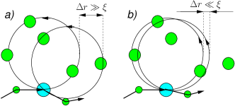
Figure 3: a) Pair of typical semiclassical trajectories and; b) of those contributing to the classical memory effect.

The case of weak magnetic field such that only single turn trajectories remain $1/\tau_{tr}\ll\omega_{c}\ll 1/\tau_{q}$, requires additional consideration, even if the criteria (30) is satisfied. The trajectories close to each other, shown in Fig. 3b, give the main contribution to the interference of return trajectories, even though the fraction of these non-typical trajectories is small. Indeed, these trajectories travel through the same disorder. The scattering off the same disorder does not randomize the sign of the product $\mbox{$\mathrm{R}e$}(a^{<}_{1}a^{>*}_{1})$, and thus exponential estimate no longer holds. On the contrary, for $\theta\lesssim\frac{\hbar}{p_{F}\xi}$, one can roughly estimate from Fig. 3b

$$a^{<}_{1}(\theta)a^{>}_{1}(\theta)\simeq\exp\left[-\frac{2\pi}{\omega_{c}\tau_{q}}\left(\frac{\Delta\mbox{\boldmath$r$}}{\xi}\right)^{2}\right],$$

where $\Delta\mbox{\boldmath$r$}$ is the typical distance between trajectories. Estimating $|\Delta\mbox{\boldmath$r$}|\simeq R_{c}\theta_{1}$, one finds for the angular interval of non-typical trajectories

$$\begin{split}\theta_{1}&\simeq\frac{\xi}{R_{c}}\left(\omega_{c}\tau_{q}\right)^{1/2}=\left(\frac{\hbar}{p_{F}\xi}\right)\left(\frac{\xi}{R_{c}}\right)\left(\frac{\omega_{c}\tau_{q}p_{F}^{2}\xi^{2}}{\hbar^{2}}\right)^{1/2}\\ &=\left(\frac{\hbar}{p_{F}\xi}\right)\left(\frac{\xi}{R_{c}}\right)\left(\omega_{c}\tau_{tr}\right)^{1/2}.\end{split}$$

The contribution of the scattering process to the transport scattering time (11), is proportional to $\theta_{1}^{3}$ and the typical scattering angle is $\hbar/(p_{F}\xi)$. Therefore the relative contribution to the non-typical trajectories to the change in all the dissipative processes, say resistivity, is

$$\frac{\Delta\rho_{xx}}{\rho_{xx}}\simeq\left(\frac{p_{F}\xi\theta_{1}}{\hbar}\right)^{3}=\left(\frac{\xi}{R_{c}}\right)^{3}\left(\omega_{c}\tau_{tr}\right)^{3/2}.$$ (31)

This power law dependence should replace $\exp(-\frac{2\pi}{\omega_{c}\tau_{q}})$ dependence in all the formulas obtained in the self-consistent Born approximation for $\hbar\omega_{c}\gg T$ (not containing Shubnikov - de Haas oscillatory term).

Finally, we notice that the product of two amplitudes for the electron propagation in the same disorder can be described as the classical probability of the circular path, and all the discussion can be recast into the notion of the classical memory effect (CME). It is not accidental that the estimate (31) coincides with calculation of the CME magnetoresistance mirlin1 up to numerical prefactor. Accurate calculation of the non-linear effect within CME model will not be done in the present paper. It is important to emphasize, however, that the fact that the self-consistent Born approximation has to be corrected by classical memory effect, affects only overall prefactors in the non-linear effects and do not change the basic structure of Eq. (20).memoryeffect

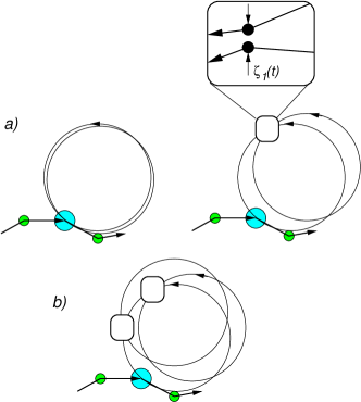
Figure 4: Trajectories with (a) two and (b) three turns contributing to the form-factors $a_{2,3}^{>}$; Inset: the semiclassical path of the electron in the vicinity of the impurity.

III Quantum Boltzmann equation (QBE)

In this section, we will derive the quantum Boltzmann equation. The propose of this derivation is to separate the contributions remaining at $\nu\gg 1$ from the very beginning. We use the standard Keldysh formalism for the non-equilibrium systemKeldysh .

III.1 Derivation of the semiclassical transport equation

The derivation is very similar to that for the Eilenberger equation Eilenberger ; 68 . The matrix Green functions and the corresponding self-energies have the form

$$\hat{G}=\begin{pmatrix}\hat{G}^{R}&\hat{G}^{K}\\ 0&\hat{G}^{A}\end{pmatrix}_{K};\quad\hat{\Sigma}=\begin{pmatrix}\hat{\Sigma}^{R}&\hat{\Sigma}^{K}\\ 0&\hat{\Sigma}^{A}\end{pmatrix}_{K},$$ (32)

where the component of the matrices are linear operators in time space and the one electron Hilbert space.

The equation for the Green function is

$$\left(i\partial_{t}-\hat{H}\right)\hat{G}=\openone+\hat{\Sigma}\hat{G};\quad\hat{G}\left(i\partial_{t}-\hat{H}\right)=\openone+\hat{G}\hat{\Sigma}.$$ (33)

where $\hat{H}$ is the one-electron Hamiltonian of the clean system, $\openone$ is the short hand notation $\openone=I_{K}\otimes I_{e}\delta\left(t_{1}-t_{2}\right)$ and $I_{K,e}$ are the unit matrices in the Keldysh space and the one electron Hilbert space respectively. [We put $\hbar=1$ in all of the intermediate formulas.] For retarded Green function we use

$$\left(i\partial_{t}-\hat{H}\right)\hat{G}^{R}=\delta(t-t_{1})\hat{I}_{e}+\hat{\Sigma}^{R}\hat{G}^{R};\quad\hat{G}^{R}\left(t<t_{1}\right)=0.$$ (34)

and $\hat{G}^{A}=\left[\hat{G}^{R}\right]^{\dagger}$. For the Keldysh Green function it is convenient to take the non-diagonal component of the difference of two Eqs. (33)

$$\left[\left(i\partial_{t}-\hat{H}\right);\hat{G}^{K}\right]=\hat{\Sigma}^{R}\hat{G}^{K}-\hat{G}^{K}\hat{\Sigma}^{A}+\hat{\Sigma}^{K}{G}^{A}-\hat{G}^{R}\hat{\Sigma}^{K},$$ (35)

where $[\cdot;\cdot]$ stands for the commutator. The next standard step is to separate the time evolution of the occupation numbers $\hat{f}$ and the wave-function of the system

$$\hat{G}^{K}=\hat{G}^{R}-\hat{G}^{A}-2\left[\hat{G}^{R}\hat{f}-\hat{f}\hat{G}^{A}\right].$$ (36)

In general $\hat{f}$ is an operator in both one-electron space and the time space. In the thermal equilibrium, however, one has simply

$$\begin{split}&\hat{f}_{F}=\int\frac{d\varepsilon}{2\pi}e^{-i\varepsilon(t_{1}-t_{2})}f_{F}(\varepsilon)=\frac{iT}{2\sinh\pi T(t_{1}-t_{2}+i0)},\\ &f_{F}(\varepsilon)=\frac{1}{e^{\varepsilon/T}+1},\end{split}$$ (37)

where $T$ is the temperature in the energy units. Substituting Eq. (36) into Eq. (35), one obtains the kinetic equation

$$\left[\left(\partial_{t}+i\hat{H}\right);\hat{f}\right]=\hat{}\mbox{St}\{\hat{f}\},$$ (38a)

with the collision integral given by

$$i\hat{}\mbox{St}\{\hat{f}\}\equiv\left[\hat{\Sigma}^{R}\hat{f}-\hat{f}\Sigma^{A}\right]+\frac{1}{2}\left[\hat{\Sigma}^{K}-\hat{\Sigma}^{R}+\hat{\Sigma}^{A}\right].$$ (38b)

Next step is to write down a self-energy for the electron subjected to the random potential $U(\mbox{\boldmath$r$})$ characterized by the correlation function

$$\langle U(\mbox{\boldmath$r$}_{1})U(\mbox{\boldmath$r$}_{2})\rangle=\int\frac{d^{2}q}{(2\pi)^{2}}W(q)e^{i\mbox{\boldmath$q$}(\mbox{\boldmath$r$}_{1}-\mbox{\boldmath$r$}_{2})}.$$

For the sake of concreteness we will adopt the model with

$$W(q)=W(0)e^{-q\xi}$$ (39)

where $\xi$ is the disorder correlation length. Equation (39) is an adequate description for the potential created by remote donors situated on the distance $\xi/2$ from the plane of two-dimensional electron gas. Self-consistent Born approximation, involving the summation of all the diagrams with non-intersecting impurity lines, see Fig. 5 is

$$\hat{\Sigma}=\int\frac{d^{2}q}{(2\pi)^{2}}W(q)\left[e^{i\mbox{\boldmath$q$}\hat{}\mbox{\boldmath$r$}}\hat{G}e^{-i\mbox{\boldmath$q$}\hat{}\mbox{\boldmath$r$}}\right].$$ (40)

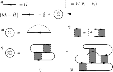
Figure 5: (a)-(b) Self-consistent Born approximation (SCBA). Diagrams (c) are most important contributions not included in the SCBA, corresponding to the logarithmically divergent second loop weak localization correctionWegner79 , see e.g. Ref. Benedict, . Diagram (c (i)) with one of the diffusons (d) reduced to one impurity line describes the first contribution to the classical memory magnetoresistancemirlin1 .

Self-consistent Born approximation is justified if two conditions

$$\xi\ll\lambda_{H},$$ (41a)

$$\sigma_{xx}\gg\frac{e^{2}}{2\pi\hbar}$$ (41b)

hold. Hereinafter $$\lambda_{H}=\left(\frac{c\hbar}{eB}\right)^{1/2} B$$ is the magnetic length, and is the applied magnetic field. The physical meaning of the condition (41a) was discussed in Sec. II, see Eq. (30). Condition (41b) allows us to neglect the localization effects shown on Fig. 5c. Note, that the external microwave radiation further suppresses the localization correctionAltshuler .

We also assume small angle scattering

$$p_{F}\xi\gg 1,$$ (42)

where $p_{F}$ is the Fermi momentum. This condition is not really essential for the physical processes but it allows for some technical simplifications. Moreover, based on Shubnikov de-Haas data, we believe that this regime is the most relevant for the experimental situation.Zudov1 ; Mani ; Zudov2

We will consider the system in the classically strong magnetic field, so that the Hall angle $\omega_{c}\tau_{tr}$ is large ($\tau_{tr}$ is the transport time, see Eq. (81) below). The effects we will be studying are proportional to the inverse Hall angle and vanish in clean systems. Therefore, it is convenient to solve time dependent problem for the clean system first, and then to consider the effect of the disorder on the top of this solution. This program is easily accomplished by using the transformation Eqs. (2) and (3). Transformation (2) removes electric field from the Hamiltonian. Instead, the disorder potential becomes time dependent. We rewrite Eq. (40) as

$$\begin{split}&\hat{\Sigma}=\int\frac{d^{2}q}{(2\pi)^{2}}W(q)e^{-i\mbox{\boldmath$q$}\mbox{\boldmath$\zeta$}_{12}}\left[e^{i\mbox{\boldmath$q$}\hat{}\mbox{\boldmath$r$}}\hat{G}e^{-i\mbox{\boldmath$q$}\hat{}\mbox{\boldmath$r$}}\right];\\ &\mbox{\boldmath$\zeta$}_{12}=\mbox{\boldmath$\zeta$}(t_{1})-\mbox{\boldmath$\zeta$}(t_{2}).\end{split}$$ (43)

Separating the guiding center coordinate and the cyclotron motion, we write

$$\hat{H}=\frac{\hat{}\mbox{\boldmath$p$}^{2}}{2m_{e}}-\mu;\quad\hat{}\mbox{\boldmath$r$}=\hat{\mbox{\boldmath$R$}}+\lambda_{H}^{2}\hat{\varepsilon}\hat{\mbox{\boldmath$p$}},$$ (44)

where $\mu$ is the chemical potential and the operators obey the following commutation relations

$$\left[\hat{R}_{\alpha};\hat{R}_{\beta}\right]=i\lambda_{H}^{2}\varepsilon_{\alpha\beta};\ \left[\hat{p}_{\alpha};\hat{p}_{\beta}\right]=-\frac{i}{\lambda_{H}^{2}}\varepsilon_{\alpha\beta};\ \left[\hat{\mbox{\boldmath$R$}};\hat{\mbox{\boldmath$p$}}\right]=0.$$ (45)

The Green functions $\hat{G}(\hat{}\mbox{\boldmath$p$};\hat{}\mbox{\boldmath$R$})$ and the self-energies $\hat{\Sigma}(\hat{}\mbox{\boldmath$p$};\hat{}\mbox{\boldmath$R$})$ can be obviously written as functions of the operators (45). Using commutation relations (45), we obtain from Eq. (43)

$$\begin{split}&\hat{\Sigma}\left(\hat{}\mbox{\boldmath$p$};{\hat{}\mbox{\boldmath$R$}}\right)=\int\frac{d^{2}q}{(2\pi)^{2}}W_{12}\left[e^{i{\bf q}\varepsilon\hat{\bf p}\lambda_{H}^{2}}\hat{G}\left(\hat{}\mbox{\boldmath$p$};{\hat{}\mbox{\boldmath$R$}}(\mbox{\boldmath$q$})\right)e^{-i{\bf q}\varepsilon\hat{\bf p}\lambda_{H}^{2}}\right]\\ &W_{12}\equiv W(q)e^{-i\mbox{\boldmath$q$}\mbox{\boldmath$\zeta$}_{12}};\quad{\hat{}\mbox{\boldmath$R$}}(\mbox{\boldmath$q$})={\hat{}\mbox{\boldmath$R$}}+\lambda_{H}^{2}\hat{\varepsilon}\mbox{\boldmath$q$}.\end{split}$$ (46)

Here we suppressed time indices.

Next step is to separate the motion in the phase space into components parallel and perpendicular to the Fermi surface. For this purpose, we parameterize the cyclotron motion operators as

$$\begin{split}&\hat{p}_{x}=\frac{1}{\lambda_{H}}\left(\frac{{N+\hat{n}}}{{2}}\right)^{1/2}e^{i\hat{\varphi}}+h.c.;\\ &\hat{p}_{y}=\frac{-i}{\lambda_{H}}\left(\frac{{N+\hat{n}}}{{2}}\right)^{1/2}e^{i\hat{\varphi}}+h.c,\end{split}$$ (47)

where the integer

$$N={\rm Int}\frac{\mu}{\omega_{c}}$$

is introduced for convenience. To preserve the commutation relations (45) for operators (47), the commutation relation

$$\left[\hat{n};\hat{\varphi}\right]=-i$$ (48)

is imposed. It follows from Eqs. (48) and (47) that the integer eigenvalues $n\geq-N$ of the operator $\hat{n}$ have the meaning of the Landau level indices. The Hamiltonian (44) acquires the form

$$\hat{H}=\omega_{c}\left[\hat{n}+\delta(\mu)\right];\ \delta(\mu)=\frac{1}{2}+N-\frac{\mu}{\omega_{c}}.$$ (49)

All the previous manipulations were valid for any magnetic field. Now we are going to make use of the large filling factor

$$N\gg 1.$$ (50a)

We will assume that the characteristic value of $$\hat{n} \parallel\hat{n}\parallel\ll N$$ contributing to the transport quantities is such that , i.e. all the relevant dynamics occurs in the vicinity of the Fermi level. This assumption is justified provided that two conditions

$$T\ll N\hbar\omega_{c};\quad\omega_{c}\tau_{q}\ll N$$ (50b)

are satisfied, with $$\tau_{q}$$ being the quantum elastic scattering time, see below. Those assumptions allow for the semiclassical consideration of the self-energy (43), which is presented below.

Using Eqs. (50), we expand Eq. (47) as

$$\begin{split}&\hat{p}_{x}=p_{F}\cos\hat{\varphi}+\frac{1}{2R_{c}}\left[\hat{n}e^{i\hat{\varphi}}+h.c.\right]+\dots;\\ &\hat{p}_{y}=p_{F}\sin\hat{\varphi}-\frac{1}{2R_{c}}\left[i\hat{n}e^{i\hat{\varphi}}+h.c.\right]+\dots,\end{split}$$ (51)

where

$$p_{F}=\frac{\sqrt{2N}}{\lambda_{H}};\quad R_{c}={\sqrt{2N}\lambda_{H}}$$

are the Fermi momentum and the cyclotron radius respectively. Substituting Eq. (51) into Eq. (46) and keeping in mind condition (42), we find

$$\begin{split}&\hat{\Sigma}\left(\hat{n};\hat{\varphi};{\hat{}\mbox{\boldmath$R$}}\right)=\int\frac{d^{2}qW_{12}}{(2\pi)^{2}}\left[\hat{U}_{\parallel}\hat{U}_{\perp}\hat{G}\left(\hat{n};\hat{\varphi};{\hat{}\mbox{\boldmath$R$}}(\mbox{\boldmath$q$})\right)\hat{U}_{\perp}^{\dagger}\hat{U}_{\parallel}^{\dagger}\right],\\ &\hat{U}_{\perp}=\exp\left[iqR_{c}\sin\hat{\varphi}_{q}-\frac{iq^{2}R_{c}\sin 2\hat{\varphi}_{q}}{4p_{F}}+{\cal O}\left(\frac{q^{3}R_{c}}{p_{F}^{2}}\right)\right],\\ &\hat{U}_{\parallel}=\exp\left\{\frac{q\left[\hat{n}e^{i\hat{\varphi}_{q}}-h.c.\right]}{2p_{F}}\right\},\quad\hat{\varphi}_{q}\equiv\hat{\varphi}-\phi_{q},\end{split}$$ (52)

where $\mbox{\boldmath$q$}=q(\cos\phi_{q};\sin\phi_{q})$. Matrix $\hat{U}_{\perp}$ commutes with $\hat{\varphi}$, i.e. in semiclassical sense it describes the scattering of the electron perpendicular to the Fermi surface. On the other hand, matrix $\hat{U}_{\parallel}$ changes $\hat{\varphi}$, i.e. it has the semiclassical meaning of the evolution parallel to the Fermi surface. Due to the condition (50a) those processes originate from parametrically different values of $q$ and that is why they can be considered separately. We use the parameterization

$$G\left(\hat{n},\hat{\varphi}\right)=\int_{0}^{2\pi}\frac{d\theta}{2\pi}e^{-i\theta\hat{n}}\tilde{G}\left(\theta,\hat{\varphi}\right).$$ (53)

Commutation relation (48) gives

$$e^{ix\sin\hat{\varphi}}e^{-i\theta\hat{n}}=e^{-i\theta\hat{n}}e^{ix\sin(\hat{\varphi}+\theta)}.$$

Thus, using definitions of Eq. (52) we obtain

$$\begin{split}&\hat{U}_{\perp}\hat{G}\left(\hat{n};\hat{\varphi};{\hat{}\mbox{\boldmath$R$}}(\mbox{\boldmath$q$})\right)\hat{U}_{\perp}^{\dagger}=\int_{0}^{2\pi}\frac{d\theta}{2\pi}e^{-i\theta\hat{n}}\tilde{G}\left(\theta,\hat{\varphi}\right)\\ &\quad\times\exp\Bigg{\{}iqR_{c}\left[\sin(\hat{\varphi}_{q}+\theta)-\sin\hat{\varphi}_{q}\right]\\ &\quad-\frac{iq^{2}R_{c}[\sin(2\hat{\varphi}_{q}+2\theta)-\sin 2\hat{\varphi}_{q}]}{4p_{F}}\Bigg{\}}\end{split}$$ (54)

The characteristic values of $q$ entering into the integral can be estimated as $qR_{c}\simeq R_{c}/\xi\gg R_{c}/\lambda_{H}=\sqrt{2N}\gg 1$. Let us call the argument of the exponent $\beta(\theta,\phi)$. Because, $qR_{c}\gg 1$, the integrals will be determined by the saddle point determined by $\beta^{\prime}_{\theta}(\theta,\phi)=0$, and $\beta^{\prime}_{\phi}(\theta,\phi)=0$ the latter condition gives $\theta=0$. Thus, we write

$$e^{i\beta(\theta,\phi)}\approx{2\pi}\delta(\theta)\delta\left[\beta^{\prime}_{\theta}(\theta,\phi)\right],$$

in a sense that the saddle point integration on the LHS gives the same result as the integration in the RHS. Employing this approximation in Eq. (54) and taking into account $\parallel\hat{n}\parallel\ll qR_{c}$,

$$\hat{U}_{\perp}\hat{G}\left(\hat{n};\hat{\varphi}\right)\hat{U}_{\perp}^{\dagger}=\frac{\tilde{G}\left(0,\hat{\varphi}\right)}{{qR_{c}}}\delta\left(\cos\hat{\varphi}_{q}-\frac{q\cos 2\hat{\varphi}_{q}}{2p_{F}}\right),$$ (55)

where $\delta-$function has to be understood in an operator sense.

We substitute Eq. (55) into Eq. (52) and use Eq. (53) to find $\tilde{G}(\theta=0)$. With the help of the commutation relation (48) and using the small angle scattering condition (42), we obtain

$$\begin{split}\hat{\Sigma}\left(\hat{\varphi};{\hat{}\mbox{\boldmath$R$}}\right)&=\frac{-i}{2\pi\mbox{\boldmath$v$}_{F}}\int_{-\infty}^{\infty}\frac{dq}{2\pi}W(q)\exp\left[-iq\mbox{\boldmath$\zeta$}_{12}\cdot\hat{\varepsilon}\mbox{\boldmath$i$}_{q}\right]\\ &\times\hat{g}\left[\hat{\varphi}+\frac{q}{p_{F}};{\hat{}\mbox{\boldmath$R$}}-\lambda_{H}^{2}q\mbox{\boldmath$i$}_{q}\right]\\ \mbox{\boldmath$i$}_{q}&\equiv\left[\cos\left(\hat{\varphi}+\frac{q}{2p_{F}}\right),\,\sin\left(\hat{\varphi}+\frac{q}{2p_{F}}\right)\right],\end{split}$$ (56)

where we introduced the analog of the Green function in the Eilenberger equation

$$\hat{g}\left(\hat{\varphi};{\hat{}\mbox{\boldmath$R$}}\right)=i\omega_{c}\sum_{k}\hat{G}\left(\hat{n}+k;\hat{\varphi};{\hat{}\mbox{\boldmath$R$}}\right).$$ (57)

Notice, that operator $\hat{\varphi}$ commutes with all other operators entering into Eq. (56), and, therefore, it can be treated as a $c$-number.

Equation (56) also can be rewritten in a different form

$$\hat{\Sigma}_{t,t^{\prime}}=-i\hat{\cal K}_{t,t^{\prime}}\hat{g}(t,t^{\prime};\varphi,{\hat{}\mbox{\boldmath$R$}}),$$ (58)

where the kernel ${\cal K}_{t,t^{\prime}}$ is

$${\cal K}_{t,t^{\prime}}=\int\frac{W(q)}{4\pi^{2}v_{F}}\exp\left[\frac{q\partial_{\varphi}}{2p_{F}}\right]e^{-iq\mbox{\boldmath$P$}\mbox{\boldmath$i$}(\varphi)}\exp\left[\frac{q\partial_{\varphi}}{2p_{F}}\right]dq,$$ (59)

with

$$\mbox{\boldmath$P$}=\mbox{\boldmath$\zeta$}_{t,t^{\prime}}\hat{\varepsilon}-i\lambda_{H}^{2}{\mbox{\boldmath$\nabla$}_{\mbox{\boldmath$R$}}}$$ (60)

This form is more convenient for the further expansion in $1/\xi p_{F}$, as we show later.

Closing this subsection we write down the expressions for the variation of the electron density, $\delta N_{e}$, and the current density, $j$. Representing the coordinate operators by Eq. (44) and approximating the operators with the help of Eq. (51) we obtain

$$\begin{split}&\delta N_{e}\left(\mbox{\boldmath$r$},t\right)=-m_{e}\int\limits_{0}^{2\pi}\frac{d\varphi}{2\pi}\delta g^{K}\left[t,t;\varphi,\mbox{\boldmath$r$}_{g}\right];\\ &\mbox{\boldmath$r$}_{g}=\mbox{\boldmath$r$}-R_{c}\hat{\varepsilon}\mbox{\boldmath$i$}(\varphi)-\mbox{\boldmath$\zeta$}(t),\end{split}$$ (61a)

and $$\delta g^{K} \mbox{\boldmath$\zeta$}(t)$$ denotes the deviation of the Keldysh Green function from its equilibrium value in the absence of the external fields. The coordinate is defined in Eq. (3).

For the full electric current we have

$$\begin{split}&\mbox{\boldmath$j$}(\mbox{\boldmath$r$},t)=eN_{e}\left(\mbox{\boldmath$r$},t\right)\partial_{t}\mbox{\boldmath$\zeta$}+\mbox{\boldmath$j$}^{(d)}(\mbox{\boldmath$r$},t),\end{split}$$ (61b)

where the first term in the current is dissipationless. At constant electric field it is nothing but the Hall current. The second term is given by

$$\begin{split}&\mbox{\boldmath$j$}^{(d)}(\mbox{\boldmath$r$},t)=-ep_{F}\int\limits_{0}^{2\pi}\frac{d\varphi}{2\pi}\mbox{\boldmath$i$}(\varphi)g^{K}\left[t,t;\varphi;\mbox{\boldmath$r$}_{g}\right].\end{split}$$ (61c)

The numerical coefficients in Eqs. (61a) and (61c) are written with account of the spin degeneracy, and $N_{e}$ is the total electron density.

III.2 Equation for the spectrum

In this subsection we solve equation (34) with the Hamiltonian (49) and the semiclassical self-energy (56)

$$\begin{split}&\left\{i\partial_{t}-\omega_{c}\left[\hat{n}+\delta(\mu)\right]\right\}G^{R}\left(t,t_{1};\hat{n}\right)=\frac{\delta(t-t_{1})}{2\pi}\\ &+\int_{t_{1}}^{t}dt_{2}\Sigma^{R}\left(t,t_{2}\right)G^{R}\left(t_{2},t_{1};\hat{n}\right).\end{split}$$ (62)

Hereinafter, we suppress $\varphi$ and $R$ arguments in the Green function and the self-energy whenever they are the same in the both sides of the equations. Our purpose is to represent the $G^{R}$ in terms of the Green functions (57) only.

For the calculation of the spectrum it is sufficient to keep the terms only to the zeroth order in small parameter $q/p_{F}$. Equations (56) and (58) then simplify to

$$\begin{split}i\hat{\Sigma}^{R}\left(\hat{\varphi};{\hat{}\mbox{\boldmath$R$}}\right)&=h_{1}\left[\frac{\left(\mbox{\boldmath$\zeta$}_{12}\hat{\varepsilon}-i\lambda_{H}^{2}\mbox{\boldmath$\nabla$}_{R}\right)\cdot\mbox{\boldmath$i$}(\varphi)}{\xi}\right]\frac{\hat{g}^{R}\left[\hat{\varphi};{\hat{}\mbox{\boldmath$R$}}\right]}{\tau_{q}}.\end{split}$$ (63)

Here

$$\frac{1}{\tau_{q}}=\frac{1}{2\pi v_{F}}\int\frac{dq}{2\pi}W(q);$$ (64)

is nothing but the standard Born approximation for the quantum scattering time for small angle scatterers, and the dimensionless function

$$h_{1}\left(x\right)=\frac{\int{dq}W(q)e^{iqx\xi}}{\int{dq}W(q)}=\frac{1}{1+x^{2}}$$ (65)

characterizes the effect of the external electric field during the cyclotron motion between electron returns to the same impurity.

We will look for the self-energy in the form

$$i\Sigma^{R}(t,t_{1})=\frac{\delta\left(t-t_{1}\right)}{2\tau_{q}}+\sum_{l=1}^{\infty}\lambda^{l}{\cal S}^{R}_{l}\left(\hat{\cal T}^{l}t\right)\delta\left(\hat{\cal T}^{l}t-t_{1}\right),$$ (66)

where the coherence factor $\lambda$ describes the phase accumulation during one period and it is defined as

$$\lambda=\exp\left(-\frac{\pi}{\omega_{c}\tau_{q}}-i2\pi\delta(\mu)\right),$$ (67)

and ${\cal S}^{R}_{l}$ are to be found self-consistently. The time shift operator is defined as

$$\hat{\cal T}^{l}t=t-\frac{2\pi l}{\omega_{c}}.$$ (68)

We look for the solution of Eq. (62) in the form

$$\begin{split}&iG^{R}\left(t,t_{1};\hat{n},\hat{\varphi}\right)=\frac{e^{-i\omega_{c}\delta(\mu)\left(t-t_{1}\right)}e^{-\frac{t-t_{1}}{2\tau_{q}}}}{2\pi}\\ &\quad\times\sum_{l}\Bigg{\{}\left[e^{-i\omega_{c}\hat{n}\,t}{\cal G}^{R}_{l}\left(\hat{\cal T}^{l}t,t_{1},\hat{\varphi}\right)e^{i\omega_{c}\hat{n}\,t_{1}}\right]\\ &\quad\times\theta\left(\hat{\cal T}^{l}t-t_{1}\right)\theta\left(t_{1}-\hat{\cal T}^{l+1}t\right)\Bigg{\}}.\end{split}$$ (69)

Substituting Eqs. (69) and (66) into Eq. (62), and using $e^{i2\pi l\hat{n}}=1$, $e^{ix\hat{n}}\varphi e^{-ix\hat{n}}=\varphi+x$ we obtain the chain of equations

$$\begin{split}&{\cal G}^{R}_{l}\left(t,t_{1};\hat{\varphi}\right)=g^{R}_{l}\left(t_{1};\hat{\varphi}\right)\\ &-\int\limits_{t_{1}}^{t}dt_{2}\sum_{m=1}^{l}{\cal S}^{R}_{m}\left[{\cal T}^{m-l}t_{2};\hat{\varphi}+\omega_{c}\left(t_{2}-t_{1}\right)\right]{\cal G}^{R}_{l-m}\left(t_{2},t_{1};\hat{\varphi}\right)\end{split}$$ (70)

where

$$\begin{split}&g^{R}_{l}\left(t;\hat{\varphi},{\hat{}\mbox{\boldmath$R$}}\right)\equiv{\cal G}^{R}_{l}\left(t,t;\hat{\varphi},{\hat{}\mbox{\boldmath$R$}}\right);\\ &{\cal G}^{R}_{l}\left(t,t_{1}\right)={\cal G}^{R}_{l-1}\left(\hat{\cal T}t,t_{1}\right);\end{split}$$ (71)

with the initial condition ${g}_{0}^{R}=1$.

Final step is the self-consistency procedure which amounts into substitution of Eq. (69) into Eq. (57). It gives :

$$\begin{split}&g^{R}\left(t;t_{1}\right)=\frac{\delta(t-t_{1})}{2}+\sum_{l=1}^{\infty}\lambda^{l}g^{R}_{l}\left(t_{1}\right)\delta\left(\hat{\cal T}^{l}t-t_{1}\right),\end{split}$$ (72)

where $\lambda$ is defined in Eq. (67). Using Eq. (72) in Eq. (63) and extracting ${\cal S}_{l}$ of Eq. (66), we find

$${\cal S}_{l}^{R}\left(t,\varphi\right)=h_{1}\left[\frac{\left(\mbox{\boldmath$\zeta$}_{l}(t)\hat{\varepsilon}-i\lambda_{H}^{2}\mbox{\boldmath$\nabla$}_{R}\right)\cdot\mbox{\boldmath$i$}(\varphi)}{\xi}\right]\frac{g^{R}_{l}\left(t,\varphi\right)}{\tau_{q}}.$$ (73)

We use the short hand notation

$$\mbox{\boldmath$\zeta$}_{l}(t)\equiv\mbox{\boldmath$\zeta$}\left(\hat{\cal T}^{-l}t\right)-\mbox{\boldmath$\zeta$}\left(t\right),$$ (74)

where the finite time shift operator is defined in Eq. (68).

Equations (70) – (73) constitute a complete system for the spectrum averaged over disorder. Note, that the Green function ${\cal G}_{l}$ is expressed in terms of ${\cal G}_{m}$ with $m<l$ only.

III.3 Equation for the distribution function

In this subsection we will reduce Eqs. (38) to the canonical Boltzmann form. According to Eq. (56) the self-energies $\hat{\Sigma}$ do not depend on $\hat{n}$. It suggests that the distribution function $\hat{f}$ does not depend on $\hat{n}$ either. This observation enables us to substitute Eq. (36) into Eq. (57) and perform the summation over $k$ with the help of Eq. (72) and relations $g^{A}=-\left[g^{R}\right]^{\dagger},\ f=f^{\dagger}$. We find

$$\begin{split}\frac{1}{2}\left[g^{R}-g^{A}-g^{K}\right]_{t,t^{\prime}}=f\left(t,t^{\prime};\varphi,\mbox{\boldmath$R$}\right)+&\sum_{l=1}^{\infty}\lambda^{l}g^{R}_{l}\left(\hat{\cal T}^{l}t;\varphi,\mbox{\boldmath$R$}\right)f\left(\hat{\cal T}^{l}t,t^{\prime},\varphi,\mbox{\boldmath$R$}\right)\\ &\quad+\sum_{l=1}^{\infty}\left(\lambda^{l}\right)^{*}f\left(t,\hat{\cal T}^{l}t^{\prime},\varphi,\mbox{\boldmath$R$}\right)\left[g^{R}_{l}\left(\hat{\cal T}^{l}t^{\prime};\varphi,\mbox{\boldmath$R$}\right)\right]^{\dagger},\end{split}$$ (75)

where the coherence factor $\lambda$ is defined in Eq. (67), and the time shift operator is given by Eq. (68).

Substitution of Eq. (75) into Eqs. (61a) and (61c) yields the connection between the distribution function $f$ and the observables:

$$\begin{split}&\delta N_{e}\left(\mbox{\boldmath$r$},t\right)=2m_{e}\int\limits_{0}^{2\pi}\frac{d\varphi}{2\pi}\Bigg{\{}\delta f\left(t,t;\varphi,\mbox{\boldmath$r$}_{g}\right)+2\mbox{$\mathrm{R}e$}\sum_{l=1}^{\infty}\lambda^{l}g^{R}_{l}\left(\hat{\cal T}^{l}t;\varphi,\mbox{\boldmath$r$}_{g}\right)f\left(\hat{\cal T}^{l}t,t;\varphi,\mbox{\boldmath$r$}_{g}\right)\Bigg{\}};\end{split}$$ (76a)

$$\begin{split}&\mbox{\boldmath$j$}^{(d)}(\mbox{\boldmath$r$},t)=2ep_{F}\int\limits_{0}^{2\pi}\frac{d\varphi}{2\pi}\mbox{\boldmath$i$}(\varphi)\Bigg{\{}f\left(t,t;\varphi,\mbox{\boldmath$r$}_{g}\right)+2\mbox{$\mathrm{R}e$}\sum_{l=1}^{\infty}\lambda^{l}g^{R}_{l}\left(\hat{\cal T}^{l}t;\varphi,\mbox{\boldmath$r$}_{g}\right)f\left(\hat{\cal T}^{l}t,t;\varphi,\mbox{\boldmath$r$}_{g}\right)\Bigg{\}},\end{split}$$ (76b)

where we used the short hand notation $$\mbox{\boldmath$r$}_{g}=\mbox{\boldmath$r$}-R_{c}\hat{\varepsilon}\mbox{\boldmath$i$}(\varphi)-\mbox{\boldmath$\zeta$}(t).$$

To derive the kinetic equation, we substitute $f$ into Eqs. (38). Equation (38a) gives

$$\left[\frac{\partial}{\partial t}+\frac{\partial}{\partial t^{\prime}}+\omega_{c}\frac{\partial}{\partial\varphi}\right]f\left(t,t^{\prime};\varphi,\mbox{\boldmath$R$}\right)=\hat{}\mbox{St}\{\,f\}_{t,t^{\prime}}.$$ (77a)

According to Eq. (38b), the collision integral is defined in terms of the electron self-energy, the latter is given by Eq. (58). Substituting Eq. (58) into Eq. (38b) and using the relation Eq. (75), we obtain the following expression for the collision integral:

$$\begin{split}\mbox{St}\{f\}_{t,t^{\prime}}=&-\left\{\hat{\cal K}(t,t^{\prime})f\left(t,t^{\prime}\right)\right\}\\ &+\sum_{l=1}^{\infty}\lambda^{l}\Bigg{\{}\left[\hat{\cal K}(t,\hat{\cal T}^{l}t)g^{R}_{l}\left(\hat{\cal T}^{l}t\right)\right]f\left(\hat{\cal T}^{l}t,t^{\prime}\right)-\left[\hat{\cal K}(t,t^{\prime})f\left(\hat{\cal T}^{l}t,t^{\prime}\right)g^{R}_{l}\left(\hat{\cal T}^{l}t\right)\right]\Bigg{\}}\\ &-\sum_{l=1}^{\infty}(\lambda^{*})^{l}\Bigg{\{}f\left(t,\hat{\cal T}^{l}t^{\prime}\right)\left[\hat{\cal K}(\hat{\cal T}^{l}t^{\prime},t^{\prime})g^{A}_{l}\left(\hat{\cal T}^{l}t^{\prime}\right)\right]-\left[\hat{\cal K}(t,t^{\prime})f\left(t,\hat{\cal T}^{l}t^{\prime}\right)g^{A}_{l}\left(\hat{\cal T}^{l}t^{\prime}\right)\right]\Bigg{\}},\end{split}$$ (77b)

In Eq. (77b) kernel $\hat{\cal K}$ is given by Eq. (59), functions $g_{l}^{R,A}$ are defined in the previous subsection by Eq. (83), the coherence factor $\lambda$ is defined in Eq. (67), and the time shift operator is defined in Eq. (68). Note that we suppressed $\varphi$ and $R$ arguments in the entries of Eqs. (77b) for brevity. The first line in Eq. (77b) corresponds to the classical scattering off an impurity; the second and the third lines describe the retarded interference corrections due to the returning orbits.

One property of the kinetic equation (77) is worth emphasizing because it is a crucial check of the consistency of the approximation we made. Consider the constant electric field $E$, so that

$$\mbox{\boldmath$\zeta$}(t)=-ct\frac{\hat{\varepsilon}\mbox{\boldmath$E$}}{B}.$$ (78)

Then the distribution function

$$f(t,t^{\prime})=f_{F}(t-t^{\prime})e^{-ie\mbox{\boldmath$E$}\hat{\mbox{\boldmath$R$}}(t-t^{\prime})}$$

where the equilibrium distribution function is given by Eq. (37), null both the collision integral and the left hand side of Eq. (77a). In the energy representation $f(\varepsilon)=f_{F}(\varepsilon+e\mbox{\boldmath$E$}\hat{}\mbox{\boldmath$R$})$ corresponds to the thermodynamic equilibrium of the system in the moving coordinate frame.

For the small angle scattering, see Eq. (42), we expand the rotation operator $\exp(q\partial_{\varphi}/2p_{f})$ in the powers of $q/p_{F}$ and obtain the following expression for the kernel Eq. (59):

$$\hat{\cal K}=\hat{\cal K}_{\bot}+\hat{\cal K}_{j}+\hat{\cal K}_{\varphi}+\hat{k}_{O}$$ (79)

where the first term contains only even angular harmonics:

$$\begin{split}\hat{\cal K}_{\bot}=&\frac{\left([p_{F}\mbox{\boldmath$\zeta$}_{t,t^{\prime}}\hat{\varepsilon}-iR_{c}\mbox{\boldmath$\nabla$}_{R}]\cdot\mbox{\boldmath$i$}\right)^{2}}{\tau_{tr}}\\ &\times h_{1}\left(\frac{\left(\mbox{\boldmath$\zeta$}_{t,t^{\prime}}\hat{\varepsilon}-i\lambda_{H}^{2}\mbox{\boldmath$\nabla$}_{R}\right)\cdot\mbox{\boldmath$i$}}{\xi}\right),\end{split}$$ (80a)

the second term contains odd angular harmonics:

$$\begin{split}\hat{\cal K}_{j}&=\frac{\left[R_{c}\mbox{\boldmath$\nabla$}_{R}\hat{\varepsilon}-ip_{F}\mbox{\boldmath$\zeta$}_{t,t^{\prime}}\right]\cdot\mbox{\boldmath$i$}}{\tau_{tr}}h_{2}\left(\frac{\left(\mbox{\boldmath$\zeta$}_{t,t^{\prime}}\hat{\varepsilon}-i\lambda_{H}^{2}\mbox{\boldmath$\nabla$}_{R}\right)\cdot\mbox{\boldmath$i$}}{\xi}\right)\\ &+\frac{p_{F}\xi}{\tau_{tr}}h_{3}\left(\frac{\left(\mbox{\boldmath$\zeta$}_{t,t^{\prime}}\hat{\varepsilon}-i\lambda_{H}^{2}\mbox{\boldmath$\nabla$}_{R}\right)\cdot\mbox{\boldmath$i$}}{\xi}\right)\partial_{\varphi},\end{split}$$ (80b)

and the third term represents the angular diffusion:

$$\begin{split}&\hat{\cal K}_{\varphi}=-\frac{1}{\tau_{tr}}\partial_{\varphi}h_{2}\left(\frac{\left(\mbox{\boldmath$\zeta$}_{t,t^{\prime}}\hat{\varepsilon}-i\lambda_{H}^{2}\mbox{\boldmath$\nabla$}_{R}\right)\cdot\mbox{\boldmath$i$}}{\xi}\right)\partial_{\varphi}.\end{split}$$ (80c)

The remaining term $$\hat{k}_{O} 1/(p_{F}\xi)^{2}$$ describes contributions which are of the order of smaller.

In Eqs. (80) we introduced the transport mean free time

$$\frac{1}{\tau_{tr}}=\frac{1}{4\pi v_{F}p_{F}^{2}}\int\frac{dq}{2\pi}q^{2}W(q)\simeq\frac{1}{\tau_{q}}\frac{1}{(p_{F}\xi)^{2}},$$ (81)

and the dimensionless function

$$h_{2}\left(x\right)=\frac{\int{dq}q^{2}W(q)e^{iqx\xi}}{\int{dq}q^{2}W(q)}=\frac{1-3x^{2}}{\left(1+x^{2}\right)^{3}}.$$ (82)

Function $h_{1}(x)$ is defined by Eq. (65), and $\mbox{\boldmath$i$}=\left(\cos\varphi,\sin\varphi\right)$.

Let us discuss in more details the meaning of the components of the kernel Eq. (79). The third term in Eq. (79), given by Eq. (80c), describes the angular diffusion. Its contribution to the collision integral suppresses angular harmonics of the distribution function rather than the zeroth harmonics.

The second term $\hat{\cal K}_{j}$ in Eq. (79), see Eq. (80b), represents the scattering process accompanied by simultaneous creation of odd-angular harmonics and energy shift. It is this term that is responsible for the dissipative current. When its is substituted into the collision integral Eq. (77b), the first line of the collision integral describes an instantaneous scattering and gives the classical conductivity. The second and third lines describe the interference due to the returns of the cyclotron trajectories. All non-linear effects considered in the following sections originate from the second and third lines of the collision integral Eq. (77b) with the full kernel $\hat{\cal K}$ replaced by $\hat{\cal K}_{j}$. The linear in $\partial_{\varphi}$ term in Eq. (80b) may be safely omitted since it does not give rise to any effects relevant for the future consideration. We kept it in Eq. (80b) to display explicitly that the operator $\hat{\cal K}_{j}$ is Hermitian as guaranteed by the relation

$$\frac{dh_{3}(x)}{dx}=2ixh_{2}(x).$$

Finally, the first term $\hat{\cal K}_{\bot}$ of the kernel Eq. (79), see Eq. (80a), is responsible for the evolution of the distribution function perpendicular to the Fermi surface, which does not mix angular harmonics of the distribution function with different parity. Similarly to $\hat{\cal K}_{j}$, in the first line of the collision integral Eq. (77b), $\hat{\cal K}_{\bot}$ describes the classical effect of the electric field on the electron distribution – Joule heating. The other terms in Eq. (77b) describe the returns of the cyclotron trajectories, which may result in oscillating components of the distribution function with period $\hbar\omega_{c}$.Mirlin-ac ; inelastic We remark that term Eq. (80a) of the collision integral can not be considered separately from inelastic processes such as the electron-electron and electron-phonon interactions. Indeed, taking the zeroth angular harmonics of Eqs. (77a) and (80a), one finds the correction to the distribution function, that grows infinitely in time. This is just a signature of the energy absorbed by the system from the external field. Elastic impurities alone can not stabilize the distribution function. The electron-electron interaction suppresses large deviations from the Fermi distribution with some effective $T_{eff}$ whereas the electron-phonon interaction prevents $T_{eff}$ from an infinite increase.

In the remainder of the paper we will consider only the phenomena associated with $\hat{\cal K}_{j}$, that are not sensitive to effects of the external field on the distribution function. Therefore we neglect the contribution to the collision integral Eq. (77b) originating from the term Eq. (80a) of the kernel Eq. (79). This contribution may be neglected if the energy relaxation time is small, the condition which is generally not valid. In recent preprintMirlin-ac an estimate of the contribution to the dc resistivity from oscillating component of the distribution function was presented. When inelastic processes are weak, this contribution is larger than the contributions studied in the present paper. Nevertheless, the effects considered here are robust and are described by different system parameters, therefore they deserve a separate consideration. The contribution which depends on the form of the electron distribution function will be presented elsewhere.inelastic The implicit assumption everywhere will also be $(T,T_{eff})\ll\mu$, i.e. the electron system is degenerate.

IV Linear transport

The purpose of this section is two-fold: (i) to demonstrate how the solution of the QBE is obtained for the simplest case and to reproduce relatively known results; (ii) to derive formulas for the spectrum which can be used as building blocks for consideration of more elaborate effects in the further sections.

We begin with the solution of Eq. (70) for the spectrum. In the linear regime, we can put $h_{1}=1$ in Eq. (73). After this simplifications entries of Eqs. (70) become independent of the angle $\varphi$ and time $t_{1}$. We find with the help of Eqs. (71) and (73)

$$\begin{split}&{\cal G}^{R}_{l}\left(t\right)=g^{R}_{l}-\frac{1}{\tau_{q}}\sum_{m=1}^{l}\int_{0}^{t}dt_{1}g^{R}_{m}{\cal G}^{R}_{l-m}\left(t_{1}\right),\\ &g^{R}_{l}={\cal G}^{R}_{l}\left(0\right)={\cal G}^{R}_{l-1}\left(\frac{2\pi}{\omega_{c}}\right);\end{split}$$ (83)

with the initial conditions $g^{R}_{0}=1,\ g^{R}_{-1}=0$.

Non-linear recursion relations (83) can be resolved exactly with the result

$$\begin{split}&{\cal G}_{l}(x)=\frac{L_{l}^{1}\left[(x+l)\alpha\right]}{l+1}+\frac{\alpha(1-x)L_{l-1}^{2}\left[(x+l)\alpha\right]}{l+1};\\ &g_{l}=\frac{L_{l-1}^{1}\left(l\alpha\right)}{l};\quad x=\frac{\omega_{c}t}{2\pi};\quad\alpha=\frac{2\pi}{\omega_{c}\tau_{q}},\end{split}$$ (84)

where $L_{l}^{m}(x)$ is the Laguerre polynomial mathbook .

Next step is to find the distribution function. To do so we use Eq. (37) for equilibrium distribution and solve Eq. (77a) to the leading order in $1/(\omega_{c}\tau_{tr})\ll 1$ and in the first order in $\mbox{\boldmath$\zeta$}(t)$, see Eq. (78). In this approximation only the collision term (80b) contributes. Taking the limits $t_{2}\to t_{1}-\frac{2\pi l}{\omega_{c}}$ for integer $l$, we find

$$\begin{split}2\pi\delta&f\left({\cal T}^{l}t,t;\varphi\right)=\frac{-\partial_{t}+\omega_{c}\partial_{\varphi}}{\tau_{tr}\left(\partial_{t}^{2}+\omega_{c}^{2}\right)}\Bigg{\{}\left[p_{F}\partial_{t}\mbox{\boldmath$\zeta$}(t)\cdot\mbox{\boldmath$i$}(\varphi)\right]\lambda_{l}^{*}g^{R}_{l}\\ &+\sum_{m=0,\ m\neq l}^{\infty}\frac{\left[p_{F}\mbox{\boldmath$\zeta$}_{l-m}(t)\cdot\mbox{\boldmath$i$}(\varphi)\right]\left(\lambda^{m}\right)^{*}\pi T}{\sinh\frac{2\pi^{2}T(l-m)}{\omega_{c}}}g^{R}_{m}\\ &+\sum_{m=1}^{\infty}\frac{\left[p_{F}\mbox{\boldmath$\zeta$}_{l+m}(t)\cdot\mbox{\boldmath$i$}(\varphi)\right]\lambda^{m}\pi T}{\sinh\frac{2\pi^{2}T(l+m)}{\omega_{c}}}g^{R}_{m}\Bigg{\}},\end{split}$$ (85)

where $\mbox{\boldmath$\zeta$}_{l}(t)$ is defined in Eq. (74).

Equations (84) and (85) are sufficient to calculate the linear response of the electric current Eq. (76b) to the applied electric field within the self consistent Born approximation at arbitrary temperatures and magnetic fields. First we discuss the high temperature limit, $T\gg\hbar\omega_{c}$, when the conductance is a smooth function of the applied magnetic field. Then we take into account $1/\omega_{c}$ oscillations of the conductivity which appear at $T/\omega_{c}\gg 1$ (Shubnikov–de Haas oscillations).

IV.1 $Ac$- and $dc$- transport at high temperatures

At $T\gg\omega_{c}$ only the first term in Eq. (85) remains and all other terms are exponentially suppressed. Introducing $N_{e}=p_{F}^{2}/(2\pi)$ and substituting Eqs. (84) and (85) into Eq. (76b), we find with the help of Eq. (67)

$$\begin{split}&\mbox{\boldmath$j$}^{(d)}(t)=\frac{\left(\hat{\varepsilon}\partial_{t}+\omega_{c}\right)^{2}}{(\partial_{t}^{2}+\omega_{c}^{2})^{2}}\left(\frac{e^{2}N_{e}}{m_{e}\tau_{tr}}\right)\\ &\times\Bigg{\{}\mbox{\boldmath$E$}(t)+2\sum_{l=1}^{\infty}\frac{e^{-\frac{2\pi l}{\omega_{c}\tau_{q}}}}{l^{2}}\left[L_{l-1}^{1}\left(\frac{2\pi l}{\omega_{c}\tau_{q}}\right)\right]^{2}\mbox{\boldmath$E$}\left(\hat{\cal T}^{l}t\right)\Bigg{\}},\end{split}$$ (86)

where the time finite shift operator is given by Eq. (68). First term in (86) describes usual scattering contribution and the subsequent terms result from the multiple returns to the same impurity. In the frequency representation Eq. (86) may be written as

$$\mbox{\boldmath$j$}_{\omega}^{(d)}=\hat{\sigma}^{(d)}(\omega)\mbox{\boldmath$E$}_{\omega},$$

where $\hat{\sigma}^{(d)}(\omega)$ is the conductivity tensor:

$$\begin{split}&\hat{\sigma}^{(d)}(\omega)=\frac{\left(-i\omega\hat{\varepsilon}+\omega_{c}\right)^{2}}{(\omega_{c}^{2}-\omega^{2})^{2}}\left(\frac{e^{2}N_{e}}{m_{e}\tau_{tr}}\right)\\ &\times\Bigg{\{}1+2\sum_{l=1}^{\infty}\frac{e^{-\frac{2\pi l}{\omega_{c}\tau_{q}}+i\frac{2\pi\omega l}{\omega_{c}}}}{l^{2}}\left[{L_{l-1}^{1}\left(\frac{2\pi l}{\omega_{c}\tau_{q}}\right)}\right]^{2}\Bigg{\}}.\end{split}$$ (87)

At $\omega=0$, Eq. (87) gives the non-oscillating correction to the diagonal $dc$ resistivity $\rho_{xx}$. Using $\omega_{c}\tau_{tr}\gg 1$, one writes $\rho_{xx}=\sigma_{xx}(\omega=0)\left[\rho_{xy}\right]^{2}$ and Eq. (87) yields

$$\begin{split}\rho_{xx}(B)=\rho_{D}\eta_{0}\left(\frac{2\pi}{\omega_{c}\tau_{q}}\right),\end{split}$$ (88)

where

$$\rho_{D}=\frac{m_{e}}{e^{2}N_{e}\tau_{tr}}$$ (89)

is the Drude resistivity, and

$$\eta_{0}(\alpha)=1+2\sum_{l=1}^{\infty}\frac{e^{-\alpha l}}{l^{2}}\left[{L_{l-1}^{1}\left(\alpha\right)}\right]^{2}.$$ (90)

The asymptotic behavior of Eq. (90) is

$$\eta_{0}(\alpha)=1+2\left[e^{-{\alpha}}+e^{-2\alpha}\left(1-\alpha\right)^{2}\right]+{\cal O}\left(e^{-3\alpha}\right)$$ (91)

at $\alpha\gg 1$ (weak magnetic field), and

$$\eta_{0}(\alpha)=\frac{16}{3\pi}\sqrt{\frac{1}{\alpha}}+{\cal O}\left(\sqrt{\alpha}\right),$$ (92)

at $\alpha\ll 1$ (strong magnetic field). Function $\eta_{0}(\alpha)$ together with its asymptotes is plotted in Fig. 6.

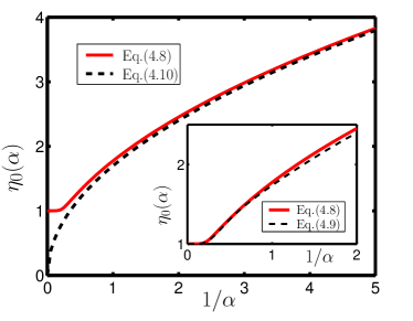
Figure 6: The solid line represents the high temperature magnetoresistance curve Eq. (88), $\alpha=2\pi/(\omega_{c}\tau_{q})$. The dashed curve in the main panel is the high field approximation (92). The dashed curve in the inset is the low-field asymptotic expression (91).

Equation (88) was written to the leading order in $1/(\omega_{c}\tau_{tr})$. To obtain the correction to the Hall coefficient one has to solve Eq. (77a) and take into account the term (80c) in the first order perturbation theory. The Hall coefficient can be expressed in terms of the third powers of the coefficients (84). The final result, however, will have the smallness $1/(\omega_{c}\tau_{tr})^{2}$ and that is why we will not write down the explicit form of those corrections. The Hall coefficient in this approximation is

$$\rho_{xy}=\frac{B}{ecN_{e}}\left[1+\frac{{\cal F}_{H}(\omega_{c}\tau_{q})}{\omega_{c}^{2}\tau_{tr}^{2}}\right]$$ (93)

where ${\cal F}_{H}(x)$ vanishes exponentially at $x\to 0$.

At finite frequency $\omega$, Eq. (86) gives, in particular, the oscillatory dependence of the absorption of microwave radiation with field $\mbox{\boldmath$E$}(t)=Re\mbox{\boldmath$E$}_{\omega}e^{-i\omega t}$ on frequency $\omega$. We find

$$\begin{split}&\mbox{$\mathrm{R}e$}\ \mbox{\boldmath$E$}^{*}_{\omega}\sigma_{xx}(\omega)\mbox{\boldmath$E$}_{\omega}=\left(\frac{e^{2}N_{e}|E_{\omega}|^{2}}{m_{e}\tau_{tr}}\right)\\ &\times\frac{\omega_{c}^{2}+\omega^{2}-2\omega\omega_{c}\cos 2\beta}{(\omega_{c}^{2}-\omega^{2})^{2}}{\cal F}_{1}\left(\frac{\omega}{\omega_{c}},\frac{2\pi}{\omega_{c}\tau_{q}}\right),\end{split}$$ (94)

where parameter $\beta$ describes the polarization of the field by parameterization of $\mbox{\boldmath$E$}_{\omega}$ as

$$\begin{split}&\frac{\sqrt{2}\mbox{\boldmath$E$}_{\omega}}{\sqrt{\mbox{\boldmath$E$}_{\omega}\cdot\mbox{\boldmath$E$}_{\omega}^{*}}}=\mbox{\boldmath$e$}_{+}\cos\beta+\mbox{\boldmath$e$}_{-}\sin\beta,\ \mbox{\boldmath$e$}_{\pm}=\mbox{\boldmath$e$}\pm i\hat{\varepsilon}\mbox{\boldmath$e$},\end{split}$$ (95)

where $e$ is the unit vector. For the circular polarization of the microwave $\beta=0,\pm\pi/2$. For the linear polarization along $e$, $\beta=\pi/4$.

The dimensionless function ${\cal F}_{1}(w,\alpha)={\cal F}_{1}(w+1,\alpha)$ represents the normalized coefficient of microwave absorption:

$${\cal F}_{1}\left(w,\alpha\right)=1+2\sum_{l=1}^{\infty}\frac{e^{-l\alpha}\cos 2\pi lw}{l^{2}}\left[L_{l-1}^{1}\left(l\alpha\right)\right]^{2}.$$ (96)

At weak field, $\alpha\gg 1$, function ${\cal F}_{1}(w,\alpha)$ is well described by the first few terms:

$${\cal F}_{1}\left(w,\alpha\right)\approx 1+2e^{-\alpha}\cos 2\pi w+2e^{-2\alpha}(1-\alpha)^{2}\cos 4\pi w+\dots.$$ (97)

At strong magnetic field, $\alpha\ll 1$, we use the asymptotic expression of the Laguerre polynomials in terms of the Bessel functions $J_{n}(y)$mathbook and obtain

$$\frac{e^{-lx/2}}{l}L_{l-1}^{1}\left(lx\right)\approx\frac{J_{1}\left(2l\sqrt{x}\right)}{l\sqrt{x}},\quad l\ll\frac{1}{x}.$$ (98)

Substituting Eq. (98) in Eq. (97) and employing the Poisson summation formula we obtain for $\alpha\ll 1$

$${\cal F}_{1}\left(w,\alpha\right)=\frac{16}{3\pi\sqrt{\alpha}}\sum_{k=-\infty}^{\infty}{\cal H}_{1}\left(\frac{\pi\left|w-k\right|}{\sqrt{\alpha}}\right)$$ (99)

where

$$\begin{split}{\cal H}&{}_{1}(x)=\frac{3\pi\theta\left(2-|x|\right)}{4}\int_{0}^{\infty}dy\cos xy\left[\frac{J_{1}(x)}{x}\right]^{2}\\ &=\frac{\left(2+x\right)\theta\left(2-|x|\right)}{8}\\ &\times\Bigg{\{}\left(4+x^{2}\right)E\left(\frac{2-x}{2+x}\right)-4xK\left(\frac{2-x}{2+x}\right)\Bigg{\}}.\end{split}$$

Functions $K(x)$ and $E(x)$ are complete elliptic integrals of the first and second kind respectively, and function ${\cal H}_{1}(x)$ can also be obtained as a convolution of two semicircle densities of states. Equation (94) and its asymptotes (97) and (99) are consistent at $|\omega-\omega_{c}|\tau_{tr}\gg 1$ with the result of recent preprint.Mirlin-ac

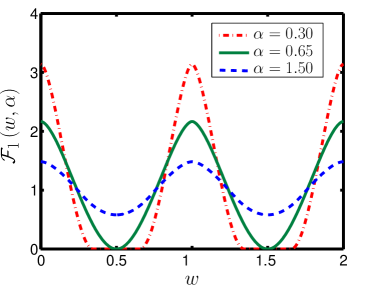
Figure 7: Dependence of normalized microwave absorption coefficient ${\cal F}_{1}(w,\alpha)$, see Eq. (96), on frequency $w=\omega/\omega_{c}$ at three values of $\alpha=\frac{2\pi}{\omega_{c}\tau_{q}}$. The function ${\cal F}_{1}(w,\alpha)$ is periodic in $w$ with the period $1$. Note, that at strong magnetic field ($\alpha=0.3$) function vanishes at intervals around $w=k+1/2$ with integer $k$.

According to Eq. (99), at sufficiently strong magnetic field the absorption coefficient ${\cal F}_{1}(w,\alpha)$ vanishes at frequency intervals such that $|w-k|>2\sqrt{\alpha}/\pi$ with integer $k$, as one may expect for the case, when the density of states has gaps between Landau levels, see e.g. Ando . Numerical investigation of ${\cal F}_{1}(w,\alpha)$ at intermediate values of $\alpha\sim 1$ allows us to find the threshold value of magnetic field, when the gap appears in the two level correlation function within the SCBA; this value of the magnetic field corresponds to $\alpha\approx 0.65$. Figure 7 shows ${\cal F}_{1}(w,\alpha)$ for three values of $\alpha$, including the threshold value $\alpha\approx 0.65$. We note that the vanishing of the two level correlation function at some energy interval is an artifact of the SCBA. However, the correction to this result (tails in the density of states) are knownEfetov to drop exponentially with the increase of the Landau level index $N$ and we disregard such tales in our study.

IV.2 $dc$ transport at low temperature

At low temperature terms in the second and third lines of Eq. (85) become important. Substitution of these terms into Eq. (76b) yields for the resistivity at $\omega_{c}\tau_{tr}\gg 1$, compare with Eq. (88),

$$\begin{split}&\frac{\rho_{xx}(B,T)}{\rho_{D}}\\ &=\sum_{l=-\infty}^{+\infty}(-1)^{l}\Upsilon\left(\frac{lT}{\hbar\omega_{c}}\right)\cos\left(\frac{\pi lp_{F}^{2}\lambda_{H}^{2}}{\hbar^{2}}\right)\eta_{l}\left(\frac{2\pi}{\omega_{c}\tau_{q}}\right),\end{split}$$ (100)

where $\rho_{D}$ is the Drude resistivity, Eq. (89), and

$$\Upsilon\left(x\right)=\frac{2\pi^{2}x}{\sinh(2\pi^{2}x)},\quad\Upsilon\left(0\right)=1.$$

The disorder dependent coefficients $\eta_{l}(\alpha)=\eta_{-l}(\alpha)$ are given by

$${\eta}_{l}\left(\alpha\right)=\sum_{k=-\infty}^{\infty}\exp\left(-\frac{\alpha(|l+k|+|k|)}{2}\right)g_{|k|}(\alpha)g_{|l+k|}(\alpha),$$ (101)

with $g_{l}(\alpha)$ defined in terms of the Laguerre polynomials by Eq. (84).

Term with $l=0$ in Eq. (100) reproduces the smooth part of the magnetoresistance (88) and $l\geq 1$ represent the Shubnikov-de Haas oscillations. The asymptotic behavior of function $\eta_{l}(\alpha)$ is the following. At low fields, $\alpha\gg 1$ only the first few terms are relevant

$$\begin{split}&\eta_{1}=2e^{-\alpha/2}+2(1-\alpha)e^{-3\alpha/2}+{\cal O}\left(e^{-5\alpha/2}\right);\\ &\eta_{2}=\left(3-2\alpha\right)e^{-\alpha}+{\cal O}\left(e^{-2\alpha}\right);\\ &\eta_{3}=\left(4-8\alpha+3\alpha^{2}\right)e^{-3\alpha/2}+{\cal O}\left(e^{-5\alpha/2}\right)\\ &\eta_{l}={\cal O}\left(\alpha^{l-1}e^{-l\alpha/2}\right).\end{split}$$ (102)

At high magnetic field $\alpha\ll 1$, we use Eq. (98) and obtain for $l\sqrt{\alpha}\ll 1$

$$\eta_{l}(\alpha)=\frac{16}{3\pi\sqrt{\alpha}}\left[1-\frac{2l^{2}\alpha}{5}+{\cal O}\left(l^{4}\alpha^{2}\right)\right].$$ (103)

Coefficients $\eta_{l}(\alpha)$ obtained from Eqs. (101) and Eq. (84) are plotted in Fig. 8.

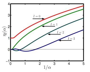
Figure 8: The harmonics $\eta_{l}$ of Shubnikov-de Haas oscillations, Eq. (100) as functions of magnetic field and the quantum scattering time, $\alpha=\frac{2\pi}{\omega_{c}\tau_{q}}$.

Below in this paper we assume that temperature is sufficiently high, $T\gg\omega_{c}$. This assumption allows us to disregard the Shubnikov–de Haas oscillations in transport quantities.

In this Section, we applied the quantum Boltzmann equation to calculate the linear response of electron system on the applied electric field. The approach developed here enabled us to describe the resistivity at arbitrary values of the parameter $\omega_{c}\tau_{q}$. Our findings are in accord with the results of Ref. Andoreview, ; Ando, ; Ando1, and differ by an overall numerical factor from the corresponding result of Ref. EAltshuler, . Particularly, the strong magnetic field asymptote for the smooth part of the magnetoresistance matches the result of Ref. Ando, . The amplitude of the Shubnikov–de Haas oscillations calculated in this Section is consistent with the previous analysis of magnetoresistance oscillations in Refs. Ando1, ; EAltshuler, . We also derived an expression for the absorption rate of microwave radiation, Eq. (94). Asymptotes of our expression in weak and strong magnetic fields coincide with the results presented in Ref. Mirlin-ac, . Having made sure that the consequences of the quantum Boltzmann equation are consistent with the results obtained by different methods, we will proceed with the description of electron transport beyond the linear response.

V Non-linear $dc$ effects

A strong $dc$ electric field produces non-linear effects on (i) the even harmonics of the distribution function, see Eq. (80a); and (ii) the elastic scattering processes (spectrum), see non-linear terms in Eq. (80b). The first mechanism roughly corresponds to the heating and it strongly affects system properties determined directly by the electron distribution function, such as Shubnikov-de Haas oscillations of the conductivity, see Sec. IV.2. As we have already noticed in Sec. III.3, the distribution function is very sensitive to the details of inelastic processes. If, however, the temperature is large,

$$T\gg\hbar\omega_{c},$$ (104)

from the very beginning we can restrict our consideration to the non-linear effects on the electron scattering process. In the remainder of the paper we consider only the high temperature limit Eq. (104).

Similarly to Eq. (85), we take into account only collision term (80b). Neglecting exponentially small terms and assuming $\omega_{c}\tau_{tr}\gg 1$, we solve Eq. (77a) and obtain

$$\begin{split}&2\pi\delta f\left({\cal T}^{l}t,t;\varphi\right)=\frac{p_{F}\partial_{\varphi}^{-1}}{\omega_{c}\tau_{tr}}\Bigg{[}\lambda_{l}^{*}g^{R}_{l}(\varphi)C\left({\cal T}^{l}t,t;\varphi\right)\Bigg{]}\\ &C\left(t_{1},t_{2};\varphi\right)=\frac{\partial}{\partial t_{2}}\left[\mbox{\boldmath$\zeta$}_{12}\cdot\mbox{\boldmath$i$}(\varphi)h_{2}\left(\frac{\mbox{\boldmath$\zeta$}_{12}\hat{\varepsilon}\mbox{\boldmath$i$}(\varphi)}{\xi}\right)\right].\end{split}$$ (105)

We notice, that the distribution function $\delta f({\cal T}^{l}t,t;\varphi)$ does not depend on time $t$. In the linear response regime $h_{2}=1$, see Eq. (82), and Eq. (105) reduces to the first term in Eq. (85).

Using Eq. (76b) and $N_{e}=p_{F}^{2}/2\pi$ we find

$$\begin{split}&\mbox{\boldmath$j$}^{(d)}=\frac{2eN_{e}}{\omega_{c}\tau_{tr}}\int\limits_{0}^{2\pi}\frac{d\varphi}{2\pi}\mbox{\boldmath$i$}(\varphi)\Bigg{\{}\partial_{\varphi}^{-1}C\left(t,t;\varphi\right)\\ &+2\sum_{l=1}^{\infty}|\lambda|^{2l}g^{R}_{l}\left(\hat{\cal T}^{l}t;\varphi\right)\partial_{\varphi}^{-1}\left[g^{R}_{l}\left(\hat{\cal T}^{l}t;\varphi\right)C\left({\cal T}^{l}t,t;\varphi\right)\right]\Bigg{\}}.\end{split}$$ (106)

Equation (106) is more complicated than its linear response counterpart, because the spectrum, determined by $g^{R}_{l}(t,\varphi)$, depends on the applied $dc$ field. It prevents one from using Eq. (84); therefore Eq. (70) should be solved again. Using Eq. (73), and Eq. (3) for the $\partial_{t}\mbox{\boldmath$E$}=0$, we obtain instead of Eq. (83)

$$\begin{split}&{\cal G}^{R}_{l}\left(t,\varphi\right)=g^{R}_{l}(\varphi)\\ &-\frac{1}{\tau_{q}}\sum_{m=1}^{l}\int_{0}^{t}dt_{1}g^{R}_{m}h_{1}\left(\frac{m\mbox{\boldmath$E$}\cdot\mbox{\boldmath$i$}(\varphi+t_{1}\omega_{c})}{E_{0}}\right){\cal G}^{R}_{l-m}\left(t_{1},\varphi\right),\\ &g^{R}_{l}={\cal G}^{R}_{l}\left(0\right)={\cal G}^{R}_{l-1}\left(\frac{2\pi}{\omega_{c}}\right);\end{split}$$ (107)

where $h_{1}$ is defined in Eq. (65), and we introduced a scale for electric field

$$E_{0}=\frac{m_{e}\omega_{c}^{2}\xi}{2\pi e}.$$ (108)

Explicit angular dependence in Eq. (107) makes the solution for an arbitrary magnetic field difficult. We consider only limiting cases of weak, $\omega_{c}\tau_{q}\ll 1$, and strong, $\omega_{c}\tau_{q}\gg 1$, magnetic fields.

At weak magnetic field, $\omega_{c}\tau_{q}\ll 1$ we can keep only first two non-trivial terms in Eq. (106). Solutions of Eq. (107) for $l=1,2$ are angular independent:

$$g_{1}=g_{0}=1;\quad g_{2}=1-\frac{2\pi}{\omega_{c}\tau_{q}}\left(\frac{E_{0}^{2}}{E^{2}+E_{0}^{2}}\right)^{1/2}.$$

Substituting these functions into Eq. (106) we obtain the solution in the form

$$\mbox{\boldmath$j$}^{(d)}=\frac{\mbox{\boldmath$E$}}{|\mbox{\boldmath$E$}|}\left(\frac{e^{2}N_{e}E_{0}}{m_{e}\omega_{c}^{2}\tau_{tr}}\right){\cal F}_{2}\left(\frac{E}{E_{0}},\frac{2\pi}{\omega_{c}\tau_{q}}\right),$$ (109)

where the dimensionless function ${\cal F}_{2}(x,\alpha)$ in the weak magnetic field can be expanded as

$$\begin{split}&{\cal F}_{2}\left(x,\alpha\gg 1\right)=x\Bigg{\{}1+\frac{2\left(1-{2x^{2}}\right)e^{-\alpha}}{\left(1+{x^{2}}\right)^{5/2}}\\ &+\frac{2\left({1}-{8x^{2}}\right)e^{-2\alpha}}{\left(1+{4x^{2}}\right)^{5/2}}\left(1-\frac{\alpha}{\left(1+x^{2}\right)^{1/2}}\right)^{2}+{\cal O}\left[e^{-3\alpha}\right]\Bigg{\}}.\end{split}$$ (110)

For the weak $dc$ fields, $|\mbox{\boldmath$E$}|\ll E_{0}$, Eq. (110) match Eq. (91).

At strong magnetic field $\omega_{c}\tau_{q}\gg 1$ the second angular harmonics in the solution of Eq. (107) is suppressed by a factor of $\alpha=2\pi/(\omega_{c}\tau_{q})$ in comparison with the zero angular harmonics. Neglecting this correction and introducing

$$\tilde{g}_{l}^{R}(E/E_{0},\alpha)=g_{l}^{R}(E/E_{0},\alpha)e^{-\alpha l/2}$$ (111)

we obtain from Eq. (107)

$$\tilde{g}^{R}_{l+1}(x,\alpha)=\left[1-\frac{\alpha}{2}\right]\tilde{g}^{R}_{l}(x,\alpha)-\alpha\sum_{m=1}^{l}\frac{\tilde{g}^{R}_{m}(x,\alpha)\tilde{g}^{R}_{l-m}(x,\alpha)}{\left(1+m^{2}x^{2}\right)^{1/2}}.$$ (112)

Equation (106) simplifies to

$${\cal F}_{2}(x,\alpha\ll 1)=x\left[1+2\sum_{l=1}^{\infty}\frac{\left(1-2l^{2}x^{2}\right)}{\left(1+l^{2}{x^{2}}\right)^{5/2}}\tilde{g}_{l}^{2}(x,\alpha)\right].$$ (113)

If the electric field is weak, $|\mbox{\boldmath$E$}|\ll\frac{E_{0}}{\left(\omega_{c}\tau_{q}\right)^{1/2}}$, one can find a solution of Eq. (112) as a correction to Eq. (84) and use approximation similar to Eq. (98):

$$\begin{split}&\tilde{g}_{l}(x,\alpha)=\sqrt{\frac{1}{\alpha l^{2}}}J_{1}\left(2\sqrt{\alpha l^{2}}\right)\Gamma_{1}\left(lx;\alpha l^{2}\right);\\ &\Gamma_{1}(x,y)=\left\{\begin{matrix}1,&y\ll 1;\\ \frac{\sqrt{1+x^{2}}}{2\sqrt{1+x^{2}}-1},&y\gg 1.\end{matrix}\right.\end{split}$$ (114)

Substituting this expression into Eq. (113), we find with the logarithmic accuracy for $x\ll 1$

$$\begin{split}{\cal F}_{2}(x,\alpha)&=\frac{x}{\pi\sqrt{\alpha}}\left[\frac{16}{3}-\frac{11x^{2}}{4\alpha}\ln\left(\frac{\alpha}{x^{2}}\right)\right].\end{split}$$ (115)

The second term in Eq. (115) represents the suppression of the renormalized transport time due to the applied electric field, compare to Eq. (92).

At strong electric field, $|\mbox{\boldmath$E$}|\gg\frac{E_{0}}{\left(\omega_{c}\tau_{q}\right)^{1/2}}$, Eq. (112) can be solved by perturbation theory in $1/(\omega_{c}\tau_{q})$

$$\tilde{g}^{R}_{l}(x,\alpha)=1-\alpha\left(\frac{l}{2}+\sum_{m=1}^{l-1}\frac{(l-m)}{\left(1+m^{2}x^{2}\right)^{1/2}}\right).$$ (116)

This gives with the help of Eq. (113) and Poisson summation formula

$${\cal F}_{2}(x,\alpha)=\frac{2\pi\alpha}{x^{2}}+\frac{8\pi^{2}}{x^{3/2}}e^{-\frac{2\pi}{x}},\quad\sqrt{\alpha}\ll x\ll 1.$$ (117)

For the strongest fields $|E|\gg E_{0}$ the main contribution to the current becomes linear in field:

$${\cal F}_{2}(x,\alpha)=x-4\frac{\zeta(3)-2\alpha\zeta(2)}{x^{2}},\quad x\gg 1,$$ (118)

where $\zeta(x)$ is the $\zeta$-function.

Dependence of ${\cal F}_{2}(x,\alpha)$ on $x$ is plotted in Fig. 9 for several values of $\alpha$. Function ${\cal F}_{2}(x,\alpha)$ is calculated according to Eq. (113) with functions $\tilde{g}_{l}(x,\alpha)$ obtained from recursive equation Eq. (112). At strong magnetic field, ${\cal F}_{2}(x,\alpha)$ exhibits a non-monotonic behavior with a minimum at $E\sim E_{0}$. At strong electric field, $E\gg E_{0}$, all curves approach the zero magnetic field result, ${\cal F}_{2}(x,\alpha)=x$, since the strong electric field destroys the interference effect of electron motion along cyclotron orbits.

Figure 10 shows the asymptotes of function ${\cal F}_{2}(x,\alpha)$ for three intervals of the strength of electric field, see Eqs. (115), (117) and (118). For comparison, we also show ${\cal F}_{2}(x,\alpha)$ calculated directly from Eq. (113) for $\alpha=1/40$.

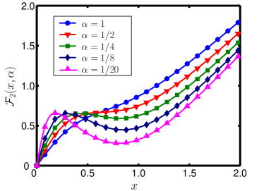
Figure 9: Nonlinear dependence of the dissipative current on the applied electric field $x=E/E_{0}$ at high-temperature $\hbar\omega_{c}\ll T$, for different values of the magnetic fields, $\alpha=2\pi/\omega_{c}\tau_{q}$.

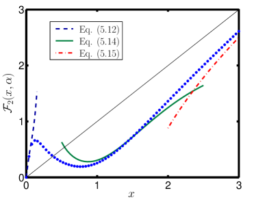
Figure 10: The plot shows three asymptotes of function ${\cal F}_{2}(x,\alpha)$ for $\alpha=1/40$: i) for small $x\ll 1$ [Eq. (115), dashed line]; ii) for $\sqrt{\alpha}\ll x\ll 1$ [Eq. (117), solid line]; iii) for large $x\gg 1$ [Eq. (118), dot-dashed line]. The dotted line represents function ${\cal F}_{2}(x,\alpha)$ at $\alpha=1/40$ calculated directly from Eq. (113).

VI Effect of microwave radiation on $dc$ transport

Consider the two-dimensional electron gas in a magnetic field $\omega_{c}\tau_{tr}\gg 1$, subjected to a monochromatic microwave radiation together with the $dc$ field

$$\mbox{\boldmath$E$}(t)=\mbox{\boldmath$E$}+\mbox{$\mathrm{R}e$}\mbox{\boldmath$E$}_{\omega}e^{-i\omega t},$$ (119)

where $\mbox{\boldmath$E$}_{\omega}$ is a complex vector in the plane of two-dimensional electron gas.

For the strong magnetic field such as the filling factor is small, $\nu\simeq 1$, the effect of microwave radiation was considered in detail in Ref. Ryzhii, , and the linear response for the short range disordered was analyzed in Ref. Durst, . Our goal is to extend these studies to the small angle impurity scattering and to the non-linear $dc$ response. The first direction will make the theory more adequate for the description of the experiments Zudov1 ; Zudov2 ; Mani ; Zudov4 , whereas the second development provides the microscopic grounds of the theory of zero-resistance state Andreev . The latter issue is analyzed in further details in the subsequent section.

To characterize the microwave power in dimensionless units, we introduce

$${\cal P}=\frac{\omega_{c}^{2}\left(\omega_{c}^{2}+\omega^{2}-2\omega\omega_{c}\cos 2\beta\right)}{2\left(\omega^{2}-\omega_{c}^{2}\right)^{2}}\left(\frac{\omega_{c}}{\pi\omega}\right)^{2}\frac{\mbox{\boldmath$E$}_{\omega}\cdot\mbox{\boldmath$E$}_{\omega}^{*}}{E_{0}^{2}},$$ (120)

where characteristic field, $E_{0}$, is defined in Eq. (108).

The polarization of the microwave is described by the angle $\beta$ and the unit vector $e$ as prescribed by Eq. (95). We will introduce also the parameter

$$\gamma(\omega)=\arctan\left(\frac{\omega+\omega_{c}}{\omega-\omega_{c}}\tan\beta\right).$$ (121)

which describes an elliptic trajectory of a classical electron in the magnetic and microwave fields.

The only difference of Eq. (122) from Eq. (105) is the time dependence of the distribution function and the spectrum due to the oscillating microwave field. Working in the approximation of large Hall angle $\omega_{c}\tau_{tr}\gg 1$ and large temperature $T\gg\hbar\omega_{c}$, we once again solve Eq. (77a) with the collision term (80b). We obtain

$$\begin{split}&\delta f\left({\cal T}^{l}t,t;\varphi\right)=\frac{p_{F}(2\pi\tau_{tr})^{-1}}{\left(\partial_{t}+\omega_{c}\partial_{\varphi}\right)}\left[\lambda_{l}^{*}g^{R}_{l}(t,\varphi)C\left({\cal T}^{l}t,t;\varphi\right)\right]\\ &C\left(t_{1},t_{2};\varphi\right)=\frac{\partial}{\partial t_{2}}\left[\mbox{\boldmath$i$}(\varphi)\mbox{\boldmath$\zeta$}(t_{1},t_{2})h_{2}\left(\frac{\mbox{\boldmath$\zeta$}(t_{1},t_{2})\hat{\varepsilon}\mbox{\boldmath$i$}(\varphi)}{\xi}\right)\right],\end{split}$$ (122)

where $\mbox{\boldmath$\zeta$}(t_{1},t_{2})\equiv\mbox{\boldmath$\zeta$}(t_{1})-\mbox{\boldmath$\zeta$}(t_{2})$ with vector $\zeta$ defined in Eq. (3), and $\lambda$ is introduced in Eq. (67). Explicitly,

$$\begin{split}\frac{\mbox{\boldmath$\zeta$}(t_{1},t_{2})}{\xi}&=\frac{\omega_{c}(t_{2}-t_{1})\hat{\varepsilon}\mbox{\boldmath$E$}}{2\pi E_{0}}+\sqrt{{\cal P}}\sin\frac{\omega(t_{2}-t_{1})}{2}\\ &\times\mbox{$\mathrm{R}e$}\left[\hat{\varepsilon}\left(\mbox{\boldmath$e$}_{+}\cos\gamma+\mbox{\boldmath$e$}_{-}\sin\gamma\right)e^{\frac{-i\omega(t_{1}+t_{2})}{2}}\right]\end{split}$$

The spectrum of the system depends both on the microwave radiation and the applied electric field. From Eqs. (70), (71), and (73) we find similarly to Eq. (107)

$$\begin{split}g^{R}_{l}(t)&={\cal G}^{R}_{l}\left(t,t\right)={\cal G}^{R}_{l-1}\left(\hat{\cal T}^{-1}t,t\right),\\ {\cal G}^{R}_{l}\left(t,t_{1},\varphi\right)&=g^{R}_{l}(t,\varphi)-\frac{1}{\tau_{q}}\sum_{m=1}^{l}\int_{0}^{t-t_{1}}dt_{2}g^{R}_{m}(t_{2},\varphi+t_{2}\omega_{c}){\cal G}^{R}_{l-m}\left(t_{2},t,\varphi\right)h_{1}\left(Z_{l,m}(t_{2},t_{1})\right),\\ Z_{l,m}(t_{2},t_{1})&=\mbox{\boldmath$i$}(\varphi+t_{2}\omega_{c})\left[\frac{m\mbox{\boldmath$E$}}{E_{0}}+\sqrt{{\cal P}}\sin\frac{\pi m\omega}{\omega_{c}}\mbox{$\mathrm{R}e$}\left(\mbox{\boldmath$e$}_{+}\cos\gamma+\mbox{\boldmath$e$}_{-}\sin\gamma\right)e^{-i\omega(t_{1}+t_{2})}e^{\frac{i\pi(m-2l)\omega}{\omega_{c}}}\right],\end{split}$$ (123)

where $h_{1}$ is defined in Eq. (65), time shift operator is given by Eq. (68), field $E_{0}$ is defined in Eq. (108), dimensionless power of the microwave radiation ${\cal P}$ is given by Eq. (120), and the angle $\gamma$ is given by Eq. (121).

We substitute the electron distribution function Eq. (122) into Eq. (76b) and obtain the following expression for the $dc$ component of the electric current in terms of $g_{l}^{R}(t,\varphi)$, compare to Eq. (106):

$$\begin{split}&\mbox{\boldmath$j$}^{(d)}=\frac{2eN_{e}}{\omega_{c}\tau_{tr}}\int\limits_{0}^{2\pi}\frac{d\varphi}{2\pi}\mbox{\boldmath$i$}(\varphi)\Bigg{\{}\partial_{\varphi}^{-1}\langle C\left(t,t;\varphi\right)\rangle_{t}+2\sum_{l=1}^{\infty}|\lambda|^{2l}\Bigg{\langle}g^{R}_{l}\left(\hat{\cal T}^{l}t;\varphi\right)\left(\partial_{t}+\omega_{c}\partial_{\varphi}\right)^{-1}\left[g^{R}_{l}\left(\hat{\cal T}^{l}t;\varphi\right)C\left({\cal T}^{l}t,t;\varphi\right)\right]\Bigg{\rangle}_{t}\Bigg{\}},\end{split}$$ (124)

and $\langle\dots\rangle_{t}$ stand for the time averaging over the period of the microwave field.

Equation (124) together with the recursion relation Eq. (123) determines the electric current to all orders both in the microwave power ${\cal P}$ and $dc$ electric field ${\bf E}/E_{0}$. We remind that our consideration is valid for large filling factors $\nu\gg 1$, large Hall angle $\omega_{c}\tau_{tr}\gg 1$, large temperatures $T\gg\hbar\omega_{c}$, and under the conditions of the applicability of self-consistent Born approximation (41). Further simplifications are possible for certain limiting cases, which will be considered below.

VI.1 Weak magnetic field, $\omega_{c}\tau_{q}\ll 1$

In this case we can limit ourselves with only first non-trivial term in Eq. (124). Because $g_{1}=1$, further calculation is reduced to straightforward angular and time integration in Eq. (124). The regimes where the compact analytic results are available are listed below.

VI.1.1 Circular polarized microwave radiation

For the linear response in $dc$ electric field ${\bf E}$, we find

$$\mbox{\boldmath$j$}^{(d)}_{c}=\left(\frac{e^{2}N_{e}\mbox{\boldmath$E$}}{m_{e}\omega_{c}^{2}\tau_{tr}}\right){\cal F}_{3}\left({\cal P},\frac{\omega}{\omega_{c}},\frac{2\pi}{\omega_{c}\tau_{q}}\right),$$ (125)

where dimensionless microwave power is defined in Eq. (120) and

$$\begin{split}{\cal F}_{3}&({\cal P},w,\alpha)=1+\frac{e^{-\alpha}\left(2-{\cal P}\sin^{2}\pi w\right)}{\left(1+{\cal P}\sin^{2}\pi w\right)^{5/2}}\\ &-\frac{3\pi w}{2}{\cal P}e^{-\alpha}\sin 2\pi w\frac{\left(4-{\cal P}\sin^{2}\pi w\right)}{\left(1+{\cal P}\sin^{2}\pi w\right)^{7/2}}+{\cal O}(e^{-2\alpha}).\end{split}$$ (126)

At ${\cal P}=0$, Eq. (126) matches Eq. (91).

Structure of Eq. (126) deserves some additional discussion. The second term in brackets describes the effect of the microwave on the elastic scattering process. In the region of the applicability of the theory $\omega_{c}\tau_{q}\ll 1$, its value can never become larger than the first term and their sum is always positive. This follows from the fact that the elastic transport cross-section is positive by construction no matter what kind of renormalization it acquires. The third term is the photovoltaic effect discussed in Sec. II. Its sign depends on the frequency of the radiation $\omega$ and, remarkably, on the power of the microwave radiation. It is noteworthy, that this term may make the current flow opposite to the electric field even at small magnetic field due to the presence of possibly large factor $6\pi\omega/\omega_{c}$ in front. Finally, we emphasize non-monotonic dependence of the photovoltaic effect on the microwave power. The frequency dependence of the $dc$ resistivity at weak field is plotted in Fig. 11. The corrections to the Hall coefficient are small as $1/(\omega_{c}\tau_{tr})^{2}$ and will net considered here explicitly.

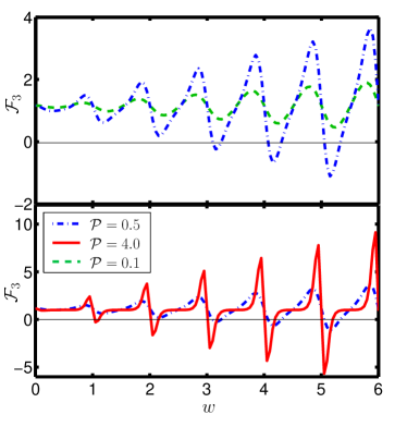
Figure 11: Frequency ($w=\omega/\omega_{c}$) dependence of ${\cal F}_{3}({\cal P},w,\alpha)$ at fixed value of the microwave power parameter ${\cal P}$ from Eq. (120) [notice, that it corresponds to the actual microwave power dependent on the frequency $\omega$] in the weak magnetic field $\omega_{c}\tau_{q}=0.8\pi$. The upper panel presents curves corresponding to the weak microwave field, ${\cal P}\lesssim 1$, whereas the solid curve in the lower panel corresponds to the strong microwave radiation ${\cal P}=4$. Curves are calculated for the circularly polarized microwave.

If the microwave power is small

$${\cal P}\sin^{2}\frac{\pi\omega}{\omega_{c}}\ll 1,$$

one can expand Eq. (126) up to the first order in ${\cal P}$. In this case, the whole non-linear $dc$ response affected by the microwave can be found, compare with Eq. (109)

$$\mbox{\boldmath$j$}^{(d)}_{c}=\frac{\bf E}{|\bf E|}\frac{e^{2}N_{e}E_{0}}{m_{e}\omega_{c}^{2}\tau_{tr}}{\cal F}_{4}\left(\frac{|\bf E|}{E_{0}},{\cal P},\frac{\omega}{\omega_{c}},\frac{2\pi}{\omega_{c}\tau_{q}}\right),$$ (127)

where

$$\begin{split}{\cal F}_{4}(x,{\cal P},w,\alpha\gg 1)&=x\Bigg{[}1+\frac{2\left(1-{2x^{2}}\right)e^{-\alpha}}{\left(1+{x^{2}}\right)^{5/2}}\\ &-3{\cal P}e^{-\alpha}\sin^{2}\pi w\frac{4-27x^{2}+7x^{4}}{2\left(1+{x^{2}}\right)^{9/2}}\\ &-3\pi w{\cal P}e^{-\alpha}\sin 2\pi w\frac{4-x^{2}}{2\left(1+x^{2}\right)^{7/2}}\\ &+{\cal O}({\cal P}^{2}e^{-\alpha})+{\cal O}(e^{-2\alpha})\Bigg{]}.\end{split}$$ (128)

Function ${\cal F}_{4}(x,{\cal P},w,\alpha)$ is plotted in Fig. 12. One can see, that at large electric field $x\gg 1$ the Ohm law is restored and the microwave radiation becomes irrelevant in accord with the conjecture of Ref. Andreev, . We will discuss consequences of negative values of ${\cal F}_{4}$ in Sec. VII.

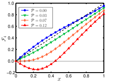
Figure 12: Non-linear dependence of ${\cal F}_{4}(x,{\cal P},w,\alpha)$ on the strength $x=|{\bf E}|/E_{0}$ of the $dc$ field for different values of power parameter ${\cal P}$ and for $\omega=7.25\omega_{c}$. Compare with Figs. 9 and 11. Curves are plotted for the regime of weak magnetic field $\omega_{c}\tau_{q}=\pi$ and for circularly polarized microwave.

At weak $dc$ field, $|E|\ll E_{0}$ one can keep only terms linear in $dc$ field in Eq. (127),

$$\begin{split}\mbox{\boldmath$j$}^{(d)}_{c}&=\left(\frac{e^{2}N_{e}\mbox{\boldmath$E$}}{m_{e}\omega_{c}^{2}\tau_{tr}}\right)\Bigg{\{}1+2e^{-\frac{2\pi}{\omega_{c}\tau_{q}}}\\ &-6{\cal P}e^{-\frac{2\pi}{\omega_{c}\tau_{q}}}\left(\sin^{2}\frac{\pi\omega}{\omega_{c}}+\frac{\pi\omega\sin\frac{2\pi\omega}{\omega_{c}}}{\omega_{c}}\right)\Bigg{\}}.\end{split}$$ (129)

It coincides with the corresponding expansion in Eq. (126).

VI.1.2 Arbitrary polarization of the microwave radiation

The compact results can be obtained for the first order expansion in ${\cal P}\sin^{2}\frac{\pi\omega}{\omega_{c}}\ll 1$. Polarization of the microwave is characterized by the parameter $\gamma$ from Eq. (121). We find

$$\mbox{\boldmath$j$}^{(d)}(\gamma)=\mbox{\boldmath$j$}^{(d)}_{c}+\delta\mbox{\boldmath$j$}_{a}\sin 2\gamma,$$ (130)

where $\mbox{\boldmath$j$}^{(d)}_{c}$ represents the isotropic component of the current and coincides with the current produced by circularly polarized microwave field, Eq. (127). The anisotropic component is given by

$$\begin{split}\delta\mbox{\boldmath$j$}_{a}&=\frac{e^{2}N_{e}E_{0}}{m_{e}\omega_{c}^{2}\tau_{tr}}\Bigg{\{}\frac{\mbox{\boldmath$E$}-2\mbox{\boldmath$e$}(\mbox{\boldmath$e$}\mbox{\boldmath$E$})}{|\mbox{\boldmath$E$}|}{\cal F}_{5}^{d}\left(\frac{|\mbox{\boldmath$E$}|}{E_{0}},{\cal P},\frac{\omega}{\omega_{c}},\frac{2\pi}{\omega_{c}\tau_{q}}\right)\\ &-\frac{\mbox{\boldmath$E$}}{|\mbox{\boldmath$E$}|}\frac{\mbox{\boldmath$E$}^{2}-2\left(\mbox{\boldmath$e$}\mbox{\boldmath$E$}\right)^{2}}{|\mbox{\boldmath$E$}|^{2}}{\cal F}_{5}^{q}\left(\frac{|\mbox{\boldmath$E$}|}{E_{0}},{\cal P},\frac{\omega}{\omega_{c}},\frac{2\pi}{\omega_{c}\tau_{q}}\right)\Bigg{\}},\end{split}$$ (131)

where functions for the dipole and quadruple angular harmonics are given by

$${\cal F}_{5}^{d}(x,{\cal P},w,\alpha)=\frac{3\pi w\sin 2\pi w}{\left(1+x^{2}\right)^{5/2}}+\frac{3(1-4x^{2})\sin^{2}\pi\omega}{\left(1+x^{2}\right)^{7/2}};$$

(132a)

$${\cal F}_{5}^{q}(x,{\cal P},w,\alpha)=\frac{15}{2}\left[\frac{\pi w\sin 2\pi w}{\left(1+x^{2}\right)^{7/2}}+\frac{(3-4x^{2})\sin^{2}{\pi\omega}}{\left(1+x^{2}\right)^{9/2}}\right]$$

for $${\cal P}\ll 1,\ \alpha\gg 1$$.

For the current linear in the $dc$ field and bilinear in the microwave field, Eq. (130) simplifies to

$$\begin{split}\delta\mbox{\boldmath$j$}_{a}&=\frac{3e^{2}N_{e}{\cal P}e^{-\frac{2\pi}{\omega_{c}\tau_{q}}}}{m_{e}\omega_{c}^{2}\tau_{tr}}\left[\mbox{\boldmath$E$}-2\mbox{\boldmath$e$}\left(\mbox{\boldmath$e$}\cdot\mbox{\boldmath$E$}\right)\right]\\ &\times\left(\frac{\pi\omega}{\omega_{c}}\sin\frac{2\pi\omega}{\omega_{c}}+\sin^{2}\frac{\pi\omega}{\omega_{c}}\right).\end{split}$$ (133)

We emphasize that the anisotropy of the electric current versus the applied electric field appears both in the linear and non-linear $dc$ transport.

In Fig. 13 we plot the $dc$ resistivity for the linear polarization, $\beta=\pi/4$, of microwave field for the cases $\mbox{\boldmath$E$}\|\mbox{\boldmath$e$}$ and $\mbox{\boldmath$E$}\bot\mbox{\boldmath$e$}$. One can see from Fig. 13 that the condition for the electric current to flow against the applied electric field $E$ depends on the polarization of the microwave field with respect to the direction of $E$.

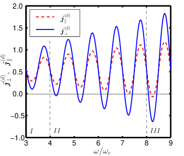
Figure 13: Dependence on microwave frequency of the electric current for a linear polarization of the microwave field: i) $\mbox{\boldmath$e$}\|\mbox{\boldmath$E$}$ (dashed line) and ii) $\mbox{\boldmath$e$}\bot\mbox{\boldmath$E$}$ (solid line). The curves are calculated for weak magnetic field $\omega_{c}\tau_{q}=\pi$ and weak power of microwave ${\cal P}=0.2$. The strength of the electric field is $|\mbox{\boldmath$E$}|=0.5E_{0}$. The plot shows that the possibility to form a current in the direction opposite to the electric field depends on the polarization of microwave field.

VI.2 Strong magnetic field, $\omega_{c}\tau_{q}\gg 1$

In this case, Eq. (123) can also be significantly simplified. We will limit ourselves with the first order expansion in microwave power ${\cal P}$.

First we analyze the first order correction in ${\cal P}$ to the spectral functions $g_{l}^{R}$ in Eq. (123). By inspection, one can see that this equation contains terms either slowly changing during the cyclotron period or oscillating with frequencies $n\omega$. The oscillating with frequency $2\omega$ term do not contribute at all to the final answer, whereas the term oscillating with frequency $\omega$ can be taken into account perturbatively. Thus, for the redefined spectral functions according Eq. (111), we obtain analogously to Eq. (112)

$$\tilde{g}^{R}_{l}(t,\varphi)=\tilde{g}^{R}_{l}+\mbox{$\mathrm{R}e$}\delta\tilde{g}_{l}(\varphi)e^{-i\omega t-i\frac{2\pi l\omega}{\omega_{c}}},$$ (134)

where the angle independent component $\tilde{g}^{R}_{l}$ satisfies the following recursion relation

$$\begin{split}\tilde{g}^{R}_{l+1}=&\tilde{g}^{R}_{l}\left[1-\frac{\pi}{\omega_{c}\tau_{q}}\right]\\ &-\frac{2\pi}{\omega_{c}\tau_{q}}\sum_{m=1}^{l}\frac{E_{0}\tilde{g}^{R}_{l-m}\tilde{g}^{R}_{m}}{\left(E_{0}^{2}+m^{2}E^{2}\right)^{1/2}}\Bigg{\{}1-{\cal P}\Xi_{1}(m)\Bigg{\}},\end{split}$$ (135)

and the angle dependent component $\delta g^{R}_{l+1}(\varphi)$ can be found from

$$\delta g^{R}_{l+1}(\varphi)=\delta g^{R}_{l}(\varphi)+\frac{2\pi\sqrt{\cal P}e^{\frac{2\pi i\omega\varphi}{\omega_{c}}}}{\omega_{c}\tau_{q}}\sum_{m=1}^{l}\Xi_{2}(m)g^{R}_{l-m}g^{R}_{m}.$$ (136)

The initial conditions for the recursion relations are $g^{R}_{0}=1,\ \delta g^{R}_{0}=0$. Above we introduced the short-hand notations

$$\begin{split}\Xi_{1}(m)&=\sin^{2}\frac{\pi m\omega}{\omega_{c}}E_{0}^{2}\\ &\times\frac{{2E_{0}^{2}}-{m^{2}\mbox{\boldmath$E$}^{2}}-3m^{2}\sin 2\gamma\left[2(\mbox{\boldmath$e$}\mbox{\boldmath$E$})^{2}-\mbox{\boldmath$E$}^{2}\right]}{4\left(E_{0}^{2}+m^{2}\mbox{\boldmath$E$}^{2}\right)^{2}}\end{split}$$ (137)

and

$$\begin{split}&\Xi_{2}(m)=\sin\frac{\pi m\omega}{\omega_{c}}E_{0}^{4}\int\limits_{0}^{2\pi}\frac{d\phi}{\pi}\exp\left(-\frac{2\pi i\omega\phi}{\omega_{c}}\right)\\ &\times\frac{\left[m\mbox{\boldmath$E$}\cdot\mbox{\boldmath$i$}(\phi)\right]\left[\left(\mbox{\boldmath$e$}_{+}\cos\gamma+\mbox{\boldmath$e$}_{-}\sin\gamma\right)\cdot\mbox{\boldmath$i$}(\phi)\right]}{\left(E_{0}^{2}+\left(m\mbox{\boldmath$i$}(\phi)\cdot\mbox{\boldmath$E$}\right)^{2}\right)^{2}},\end{split}$$ (138)

where $\gamma$ is given by Eq. (121).

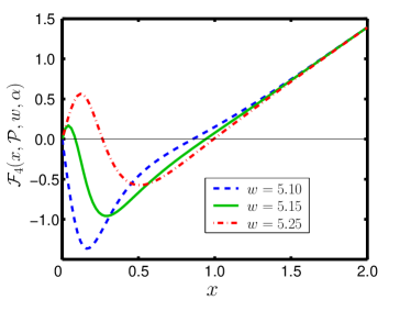
Figure 14: Nonlinear dependence of ${\cal F}_{4}$, Eq. (140), on the strength $x=|\mbox{\boldmath$E$}|/E_{0}$ of the $dc$ electric field at several values of the microwave frequency $w=\omega/\omega_{c}$ in strong magnetic field $\omega_{c}\tau_{q}=40\pi$ at ${\cal P}=0.05$.

One can see, that due to the oscillating factor $e^{\frac{2\pi i\omega\varphi}{\omega_{c}}}$ in Eq. (136) the contribution of this term is suppressed by additional factor of $\omega_{c}/\omega$ in comparison with contribution of $\Xi_{1}$ in Eq. (135). Nevertheless, even $\Xi_{1}$, which describes the effect of the microwave radiation on the density of states, is suppressed in comparison with photovoltaic effect by a factor of $\omega_{c}/\omega$. Thus, in the consideration of the transport at

$$\omega\gg\omega_{c},$$ (139)

we replace $\tilde{g}_{l}^{R}(t,\varphi)$, defined by Eq. (135), with $\tilde{g}_{l}^{R}(t,\varphi)$ obtained from Eq. (112). All the further formulas of this Section are valid in this high-frequency limit only.

We present the $dc$ current in the form of Eq. (130), where the polarization dependence is characterized by factor $\gamma$, Eq. (121). Keeping in mind condition (139), we obtain from Eqs. (122) and (124) the following expressions for the functions defined in Eqs. (127) and (131)

$$\begin{split}&{\cal F}_{4}(x,{\cal P}\ll 1,w\gg 1,\alpha\ll 1)\\ &\ \ ={\cal F}_{2}(x,\alpha)-\frac{3\pi xw{\cal P}}{2}\sum_{l=1}^{\infty}\frac{\left(4-l^{2}x^{2}\right)\sin(2\pi lw)}{(1+l^{2}x^{2})^{7/2}}\tilde{g}_{l}^{2}(x,\alpha),\end{split}$$ (140)

and

$${\cal F}_{5}^{d}(x,{\cal P},w,\alpha)={3\pi w}{\cal P}\sum_{l=1}^{\infty}\frac{l\sin 2\pi lw}{\left(1+l^{2}x^{2}\right)^{5/2}}\tilde{g}_{l}^{2}(x,\alpha);$$

(141a)

$${\cal F}_{5}^{q}(x,{\cal P},w,\alpha)=\frac{15\pi w}{2}{\cal P}\sum_{l=1}^{\infty}\frac{l^{3}\sin 2\pi lw}{\left(1+l^{2}x^{2}\right)^{7/2}}\tilde{g}_{l}^{2}(x,\alpha).$$

for ${\cal P}\ll 1,\ w\gg 1,\alpha\ll 1$ Here, the spectral functions $\tilde{g}_{l}$ are solutions of Eq. (112).

In Fig. 14 we present ${\cal F}_{4}(x,{\cal P},w,\alpha)$ as a function of the strength of the electric field $x=|\mbox{\boldmath$E$}|/E_{0}$ for several values of frequency $w=\omega/\omega_{c}$ at strong magnetic field, $\omega_{c}\tau_{q}=40\pi$. We observe that the effect of microwave field on $dc$ current is significant only in the non-linear region, $|\mbox{\boldmath$E$}|\lesssim E_{0}$. At stronger electric fields $|\mbox{\boldmath$E$}|\gg E_{0}$, the effect of microwave on the $dc$ current disappears, see Sec. II for a discussion.

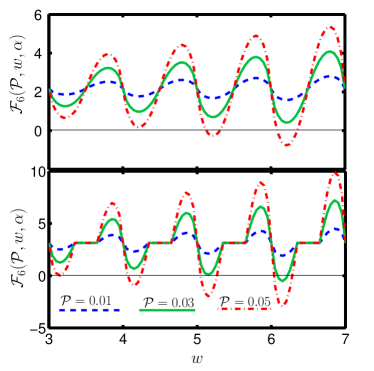
Figure 15: Dependence of ${\cal F}_{6}({\cal P},w,\alpha)$ on frequency $w=\omega/\omega_{c}$ for several values of ${\cal P}$. The upper panel represents the curves calculated for $\alpha=0.65$, and the lower panel shows the curves for $\alpha=0.30$; cf. Fig. 7.

We also calculate the $dc$ current linear in the $dc$ field $E$ and bilinear in the microwave field. For simplicity we consider only the isotropic component of the current, which survives at $\gamma=0$ in Eq. (130) and corresponds to the current produced by the circular polarization. In this case we use the spectral function $g_{l}(x,\alpha)$, given by Eq. (84) and obtain

$$\mbox{\boldmath$j$}_{c}^{(d)}=\frac{e^{2}N_{e}\mbox{\boldmath$E$}}{m_{e}\omega_{c}^{2}\tau_{tr}}{\cal F}_{6}({\cal P},w,\alpha),$$ (142)

where

$${\cal F}_{6}({\cal P},w,\alpha)=\lim_{x\to 0}\frac{{\cal F}_{4}(x,\dots)}{x}=\eta_{0}(\alpha)+\frac{3w{\cal P}}{2}\frac{\partial}{\partial w}{\cal F}_{1}(w,\alpha),$$ (143)

and functions $\eta_{0}(\alpha)$ and ${\cal F}_{1}(w,\alpha)$ are defined by Eqs. (90) and (96) respectively. Relation between the absorption spectrum and the microwave frequency dependence of the photovoltaic effect (143) was argued recently in Ref. HeandShe, on the basis of a “toy model”. Dependence of ${\cal F}_{6}({\cal P},w,\alpha)$ on frequency $w=\omega/\omega_{c}$ is shown in Fig. 15 for several values of ${\cal P}$. [Note that fixed ${\cal P}$ corresponds to the frequency dependence of the actual microwave power, see Eq. (120).]

At strong magnetic field we use Eqs. (92) and (99) to find the asymptotic form of function ${\cal F}_{6}({\cal P},w,\alpha)$ at $\alpha\ll 1$:

$${\cal F}_{6}({\cal P},w,\alpha)=\frac{16}{3\pi\sqrt{\alpha}}\left[1+\frac{3\pi}{2}\frac{{\cal P}w}{\sqrt{\alpha}}\sum_{k}{\cal H}_{2}\left(\frac{\pi|w-k|}{\sqrt{\alpha}}\right)\right],$$ (144)

where for $|x|\leq 2$

$${\cal H}_{2}(x)=\frac{3x}{8}\Bigg{\{}(2+x)E\left(\frac{2-x}{2+x}\right)-4K\left(\frac{2-x}{2+x}\right)\Bigg{\}},$$

and ${\cal H}_{2}(x)=0$ otherwise, see also discussion in the last paragraph of Sec. IV.1. Function ${\cal H}_{2}(x)$ has the minimum at $x_{min}\approx 0.834$, where ${\cal H}_{2}(x_{min})\approx 0.726$. Correspondingly, function ${\cal F}_{6}({\cal P},w,\alpha)$ becomes negative if the microwave power ${\cal P}$ exceeds ${\cal P}_{min}\approx 0.29\sqrt{\alpha}/w$ (here $\alpha\lesssim 1$ and $w\gtrsim 1$). This expression demonstrates that at strong magnetic fields, $\alpha\lesssim 1$, already a weak microwave is sufficient to create a state with zero-bias negative resistance.

VII Formation of inhomogeneous phases and current in domains

Results of the previous section qualitatively consistent with the conclusions of Ref. Ryzhii, ; Ryzhii1, ; Durst, indicate that there is a region in the parameter space where the linear dissipative conductivity becomes negative. According to Ref. Andreev, , spatially homogeneous state of such system is unstable and break itself into the domains characterized by zero dissipative resistivity and conductivity and by the classical Hall resistivity, see Fig. 16. In the analysis of such state one can ask two main questions: (i) what the spatial structure of the domain wall and the boundary conditions fixing the position and the size of the domains are; (ii) what the values of the current and the electric field inside domains are; the value of electric field can be found by the local probe measurement.

First question has to be answered by analyzing spatially inhomogeneous problem by taking into account the gradient term in Eq. (80b) and the Poisson equation; this question is left for future study. Here, we use the results of Sec. VI to address the second question.

To clarify further consideration, let us discuss the relation between applied current and voltage in more details. In all of the above analysis we assumed that the electric field $E$ is applied and the current $j$ is measured, the current has both the dissipative and Hall components; the corrections to the Hall coefficient are small as $1/(\omega_{c}^{2}\tau_{tr}^{2})$. Restoring the Hall current we write the expression for the total $dc$ current up to the terms ${\cal O}(\omega_{c}^{-2}\tau_{tr}^{-2})$

$$\mbox{\boldmath$j$}=\left(\frac{e^{2}N_{e}E_{0}}{m_{e}\omega_{c}^{2}\tau_{tr}}\right)\hat{\cal F}\left(\frac{\mbox{\boldmath$E$}}{E_{0}},{\cal P},\frac{\omega}{\omega_{c}},\frac{2\pi}{\omega_{c}\tau_{q}}\right)\frac{\mbox{\boldmath$E$}}{|\mbox{\boldmath$E$}|}-\frac{1}{\rho_{xy}}\hat{\varepsilon}\mbox{\boldmath$E$},$$ (145a)

where $\rho_{xy}$ is the classical Hall coefficient, see Eq. (93), and $\hat{\cal F}$ is the tensor defined for different situations in Eqs. (109), (127), and (131). [Tensor structure appears due to the microwave radiation with polarization other than circular, see Eqs. (130) – (133), (141). ] Microwave power is characterized by Eq. (120) and the field $E_{0}$ is given by Eq. (108). This relation is convenient to use for the Corbino disk measurement scheme. For the Hall bar geometry Eq. (145a) can be easily inverted

$$\mbox{\boldmath$E$}=-{j_{0}}{\rho_{D}}\hat{\varepsilon}\hat{\cal F}\left(\frac{\mbox{\boldmath$j$}}{j_{0}},{\cal P},\frac{\omega}{\omega_{c}},\frac{2\pi}{\omega_{c}\tau_{q}}\right)\frac{\hat{\varepsilon}\mbox{\boldmath$j$}}{|\mbox{\boldmath$j$}|}+{\rho_{xy}}\hat{\varepsilon}\mbox{\boldmath$j$},$$ (145b)

where $\hat{\varepsilon}^{2}=-1$, $\rho_{D}$ is the classical Drude resistivity (89), and

$$j_{0}=\frac{E_{0}}{\rho_{xy}}=eN_{e}\frac{\xi\omega_{c}}{2\pi}$$ (146)

is the electric current scale for non-linear effects. Equations (145) shows that both Hall bar and Corbino measurements should exhibit the similar non-linear properties, as will be discussed below.

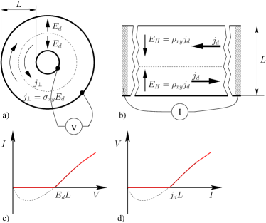
Figure 16: Domain structureAndreev for the Corbino (a) and Hall bar (b) geometries. For the Hall geometry, the applied current $I<j_{d}L$ is accommodated by the shift of the domain wall without any voltage drop, $V_{x}=0$. At $I>j_{0}L$ ($V>E_{d}$) for the Hall bar (Corbino) geometry domain structure is destroyed and the state with finite dissipation is stable (c). Note, that the construction (b) does not describe the current pattern near the leads.

We mainly focus our consideration on the circular polarization of microwave radiation; non-circular polarization is briefly discussed in the end of this section. Then, tensor $\hat{\cal F}$ from Eqs. (145) is reduced to scalar and the condition of the local stability of the state takes the formAndreev

$$j_{d}=xj_{0};\quad E_{d}=xE_{0};$$ (147a)

where $$x$$ is the solution of

$${\cal F}\left(x,{\cal P},\frac{\omega}{\omega_{c}},\frac{2\pi}{\omega_{c}\tau_{q}}\right)=0;\quad\partial_{x}{\cal F}\left(x,{\cal P},\frac{\omega}{\omega_{c}},\frac{2\pi}{\omega_{c}\tau_{q}}\right)>0.$$ (147b)

All the further analysis is reduced to the substituting of appropriate limit of the function (127) into the stability condition (147).

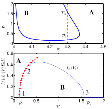
Figure 17: Upper panel: Phase diagram of a 2DEG in weak magnetic field ($\alpha=2$) in ${\cal P}-w=\frac{\omega}{\omega_{c}}$ coordinates [$I=0$ ($V=0$) for the Hall bar (Corbino) geometries]. Region (A) is the dissipative state; region (B) is the zero resistance (conductance) state. Lower panel: Phase diagram for $\omega=4.3\omega_{c}$ (dashed line on the upper panel) in ${\cal P}\!-\!{I}$ coordinates for the Hall bar (${\cal P}\!-\!{V}$ for the Corbino) geometries. The zero resistance (conductance) state exists if the current through the Hall bar (voltage drop between edges of the Corbino disk) does not exceed the critical value $I_{c}$ ($V_{c}$). The same curve defines the value of the spontaneous current $j_{d}=I_{c}/L$ (electric field $E_{d}=V_{c}/L$) in domains. The line labelled by “+” is the numerical solution of Eq. (150) and the line “2-3” is a schematic interpolation beyond the linear expansion in microwave power. Points ${\cal P}_{u,l}$ are the same as in the upper panel.

The regime of the weak magnetic field $\alpha=\frac{2\pi}{\omega_{c}\tau_{q}}\gg 1$ is simplest. According to Eq. (125), the zero current state is stable if ${\cal F}_{3}>0$, thus, the equation

$${\cal F}_{3}\left({\cal P},\frac{\omega}{\omega_{c}},\alpha\right)=0$$ (148)

gives the boundary between dissipative and zero resistance state (ZRS) for the Hall bar geometry or zero conductance state (ZCS) for the Corbino disk geometry in ${\cal P}\!-\!\omega$ plane, where ${\cal F}_{3}\left({\cal P},\frac{\omega}{\omega_{c}},\alpha\gg 1\right)$ is given by Eq. (126). The curve given by Eq. (148) is plotted in the upper panel of Fig. 17. For $w=\frac{\omega}{\omega_{c}}\gg 1$ the analytic estimates for the “phase boundary” lines are

$${\cal P}_{l} \simeq \frac{e^{\alpha}}{6\pi w\sin 2\pi w},\quad{\cal P}_{l}\ll 1;$$ (149a)

$${\cal P}_{u} \simeq \frac{4}{\sin^{2}\pi w}-5^{7/2}{\cal P}_{l},\quad{\cal P}_{u}\gg 1.$$ (149b)

The zero resistance state is impossible not only at too low microwave power but also at excessive microwave power (reentrance transition). Indeed, a weak microwave radiation does not produce strong enough photovoltaic current to compensate the dissipative current. On the other hand, as we discussed in Sec. II, strong microwave radiation suppresses the electron returns to the same impurity and thus destroys the non-linear effects.

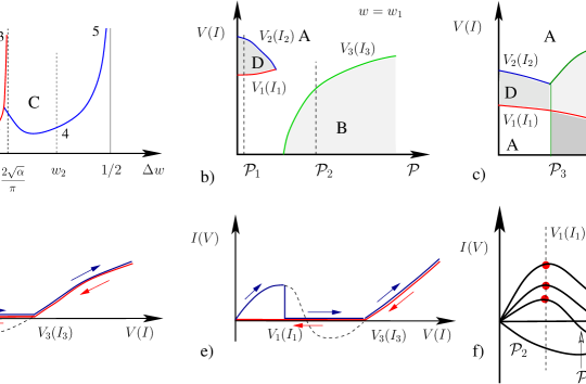
Figure 18: (a) Phase diagram of a 2DEG in strong magnetic field ($\alpha\ll 1$) in ${\cal P}-w=\frac{\omega}{\omega_{c}}$ coordinates [$I=0$ ($V=0$) for the Hall bar (Corbino) geometries]. The dissipative (A), the zero resistance (conductance) state (B) and the coexistence regions (C) are shown. (b,c) Phase diagrams for $\omega/\omega_{c}=w_{1}$ and $\omega/\omega_{c}=w_{2}$ (vertical dashed lines on the upper plane) in ${\cal P}\!-\!{I}$ coordinates for the Hall bar (${\cal P}\!-\!{V}$ for the Corbino) geometries. Lines $V_{3}(I_{3})$ also describe the current in domains as functions of the microwave power. The dissipative instability region is denoted by D. (d,e) The $I-V$, ($V-I$) characteristics for the Hall bar (Corbino disk) geometries at ${\cal P}={\cal P}_{2}$ and ${\cal P}={\cal P}_{4}$ respectively; (f) Relation of the position of the border lines to the results of Fig. 14.

At microwave power within the zero-resistance region Eq. (147b) has the solution at $x\neq 0$

$${\cal F}_{4}\left(x,{\cal P},\frac{\omega}{\omega_{c}},\frac{2\pi}{\omega_{c}\tau_{q}}\right)=0.$$ (150)

For the low microwave power response ${\cal F}_{4}$ is given by Eq. (127).

Phase boundary given by Eq. (150) is shown on the lower panel of Fig. 17 by the $1-2-3$ curve. In the vicinity of the lower boundary (segment $1-2$) and at $\omega\gg\omega_{c}$ we have

$$\begin{pmatrix}j_{d}\\ \\ E_{d}\end{pmatrix}=\begin{pmatrix}j_{0}\\ \\ E_{0}\end{pmatrix}\sqrt{\frac{4\left({\cal P}-{\cal P}_{l}\right)}{15{\cal P}_{l}}},$$ (151)

where ${\cal P}_{l}$ is given by Eq. (149a). As the power increases, the current in domains reaches maximum and then decreases. This non-monotonic behavior is schematically shown by the $1-2-3$ line in the lower panel of Fig. 17. The corresponding segment ($2-3$) may be obtained from calculations outlined in Sec. VI.1.1 beyond the bilinear response in the microwave field, which was not done in the present paper. [Based on the results presented in Sec. VI.1.1, only point $3$ of this segment is known.] However, there is no reason to expect any singular behavior of this curve.

The lower panel of Fig. 17 may be also used as a phase diagram in ${\cal P}\ -\ I$ plane, where $I=jL$ is the total current through the Hall bar of width $L$ or in ${\cal P}\ -\ V$ plane for the Corbino geometry, see Fig. 16.

We now turn to the discussion of the strong magnetic field regime $\omega_{c}\tau_{q}\gg 1$. Naively, one would expect that increase of the magnetic field would change the phase diagram of Fig. 17 only quantitatively by rearranging the boundary line. However, this expectation is not correct. We start from the phase diagram on ${\cal P}\!-\!w$ plane, Fig. 18a. The condition for the boundary between the dissipative and ZRS (ZCS) (148) is modified as

$${\cal F}_{6}\left({\cal P},\frac{\omega}{\omega_{c}},\alpha\right)=0,$$ (152)

where ${\cal F}_{6}$ is given by Eqs. (143) and (144). Solution of Eq. (152) gives the line $1-2-3$ in Fig. 18a. On can see that the region of the instability shrinks with increasing of the magnetic field. It is not the end of the story though. According to Fig. 14, see curves for $w=5.15$ and $w=5.25$, the state with positive zero-field resistance but with dissipative electric field antiparallel to the electric current at some finite current is possible. The boundary line (curve $3-2-4-5$ in Fig. 18a) for such state is given by, see also Eq. (147b)

$${\cal F}_{4}\left(x_{*},{\cal P},\frac{\omega}{\omega_{c}},\frac{2\pi}{\omega_{c}\tau_{q}}\right)=0;$$

$$\partial_{x}{\cal F}_{4}\left(x_{*},{\cal P},\frac{\omega}{\omega_{c}},\frac{2\pi}{\omega_{c}\tau_{q}}\right)=0,$$ (153)

where ${\cal F}_{4}$ is given by Eq. (140). The solution of Eq. (153) is shown as the line $2-4-5$ in Fig. 18a. Therefore, the phase diagram becomes more complicated. The region of the ZRS (ZCS) has the same properties as its counterpart for the weak field. On the other hand, in the coexistence region (C), see Fig. 18a,c, both the homogeneous dissipative state with zero current and the domain structure of the ZRS (ZCS) are locally stable. We believe that such bistability can cause the hysteretic behavior of the $I-V$ characteristic of the sample, see Fig. 18(e).

The aforementioned complication translates into the qualitative change in the phase diagrams in ${\cal P}\!-\!{V}$ (${\cal P}\!-\!{I}$) coordinates, see Fig. 18 (b,c) in comparison with the lower panel of Fig. 17. Equations for the lines on Fig. 18(b,c) are

$$\begin{matrix}\partial_{x}{\cal F}_{4}\left(x,{\cal P},\frac{\omega}{\omega_{c}},\frac{2\pi}{\omega_{c}\tau_{q}}\right)=0;&&{\rm Lines}\ \ \ V_{1,2}\ (I_{1,2})\\ {\cal F}_{4}\left(x,{\cal P},\frac{\omega}{\omega_{c}},\frac{2\pi}{\omega_{c}\tau_{q}}\right)=0;&&{\rm Line}\ \ \ V_{3}\ (I_{3}),\end{matrix}$$

and $V=xLE_{0}$ ($I=xLj_{0}$). The physical meaning of those lines is illustrated on Fig. 18f.

The region D in Fig. 18 (b,c) represents the state with negative differential conductance (for Corbino geometry). In this case, the homogeneous state is unstable, whereas the zero-resistance state is not possible. The instability of the homogeneous state, see Fig. 19 leads to the formation of the domain structure with the charge distribution similar to the Gunn domainGunn . This structure will be moving from the boundary to the boundary with the velocity $\xi\omega_{c}{\cal F}^{*}/(2\pi)$, thus the domain will be annihilated on the contact with the other one formed on the opposite contact; so that the current pattern will be oscillating in time rather than stationary.

Figure 19: The schematic picture of the current distribution in the instability region D for the Corbino geometry.

Finally, let us discuss the role of the anisotropy of the dissipative conductivity tensor in the formation of zero-resistance (conductance) state for the linear polarization of microwave. Here, two situations are possible, (i) both main components of the linear resistivity tensor are negative though different; (ii)the main components of the linear resistivity tensor are of different signs, see Fig. 13. Study of the regime (i) can be reduced to the previously studied case by rescaling of the coordinate, currents and field, such that equations $\mbox{\boldmath$\nabla$}\cdot\mbox{\boldmath$j$}=0$, $\mbox{\boldmath$\nabla$}\times\mbox{\boldmath$E$}=0$ are kept intact. It does not change the state of Ref. Andreev, qualitatively, though extra singularities may be needed to accommodate the change in the boundary conditions. For case (ii), the homogeneous state can be shown to be unstable, whereas the domain structure with closed current loops would violate the condition $\oint\mbox{\boldmath$E$}\cdot d{\bf l}=0$, because on such contour there must be regions of positive resistance. The details of current pattern for this case requires the further investigation, we believe, however, that the stationary solution for this case is not possible and domains oscillating in time will be formed.

VIII Conclusions

In this paper, we derived the kinetic equation within the self consistent Born approximation for large filling factors. The obtained equation are written in terms of the Green functions integrated in the phase space in the direction perpendicular to the Fermi surface similarly to the Eilenberger equation for normal metals and superconductors. Our system of equations takes into account the effect of electric and magnetic fields on the elastic scattering process, i.e. on both the spectral function and the electron distribution function.

Armed with the quantum kinetic equation for the limit of large Hall angle, we described the following phenomena: (i) $dc$ and $ac$ magnetoresistance in the linear response; (ii) non-linear $dc$ current-voltage characteristic; (iii) influence of oscillating microwave electric field on $dc$ current. It is important to emphasize that the non-trivial effects of the theory are described in terms of only two free parameters, time $\tau_{q}$ which can be extracted for the Shubnikov–de Haas oscillations, and the characteristic electric field $E_{0}$ from Eq. (108). The major problem of the presented paper is the lack of the consideration of the inelastic processes and consequently, effects related to the form of electron distribution function. The treatment of inelastic processes will be presented in ref. inelastic, .

We conclude by mentioning another consequence of the proposed in Ref. Andreev, domain mechanism of zero resistance (ZRS) and zero conductance states (ZRC). Namely, according to our finding, the zero dissipative current represent the interplay of two effects: elastic scattering off impurities and the photovoltaic effect; electric field in the domain is found from the condition that these two effects compensate each other on average. However, those processes are statistically independent. Consequently, this statistical independence of two processes may be revealed through the current noise in the ZRS or ZCS, which is not expected to have any singularity in this regime. The analysis of this noise can be performed by slight modification of the equations derived in the present paper in the spirit of e.g. Ref.  Agam, and left as a subject for the future research.

References

- (1) See T. Ando, A.B. Fowler, and F. Stern, Rev. Mod. Phys, 54, 437 (1982) for general review.
- (2) See The Quantum Hall Effect, R.E. Prange and S.M. Girvin (eds.), 2nd ed. (1990) for general review.
- (3) M.A. Zudov, R.R. Du, J.A. Simmons, and J.L. Reno; cond-mat/9711149; Phys. Rev. B 64, 201311(R) (2001).
- (4) R. Mani, J.H. Smet, K. von Klitzing, V. Narayanamurti, W.B. Johnson, and V. Umansky, Nature, 420, 646 (2002).
- (5) M. A. Zudov, R. R. Du, L. N. Pfeiffer, and K. W. West, Phys. Rev. Lett. 90, 046807 (2003).
- (6) R.G. Mani, J.H. Smet, K. von Klitzing, V. Narayanamurti, W.B. Johnson, and V. Umansky, cond-mat/0303034.
- (7) C.L. Yang, M.A. Zudov, T.A. Knuuttila, R.R. Du, L.N. Pfeiffer, and K.W. West, cond-mat/0303472.
- (8) S.I. Dorozhkin, JETP Lett. 77, 577 (2003) [Pis’ma ZhETF 77, 681 (2003)], cond-mat/0304604.
- (9) V.I. Ryzhii, Fiz. Tverd. Tela, 11, 2577 (1969); [Sov. Phys. Solid State, 11, 2078, (1970)].
- (10) V.I. Ryzhii, R.A. Suris, and B.S. Shchamkhalova, Fiz. Tekh. Poluprovodn. 20, 2078, (1986) [Sov. Phys. Semiconductors, 20, 1289 (1986)].
- (11) Adam C. Durst, Subir Sachdev, N. Read, and S.M. Girvin, Phys. Rev. Lett. 91, 086803 (2003).
- (12) A.V. Andreev, I.L. Aleiner, and A.J. Millis, Phys. Rev. Lett. 91, 056803 (2003).
- (13) For review, see e.g. E. Schöll. Nonlinear Spatio-Temporal Dynamics and Chaos in Semiconductors, (Cambrdige University Press, 2001).
- (14) A.L. Zakharov, Zh. Eksp. Teor. Fiz. 38, 665 (1960) [Sov. Phys. JETP, 11, 478 (1960)].
- (15) M.I. D’yakonov, Pis’ma Zh. Eksp. Teor. Fiz. 39, 158 (1984) [JETP Lett., 39, 185 (1984)]; M.I. D’yakonov and A.S. Furman, Zh. Eksp. Teor. Fiz. 87, 2063 (1984) [Sov. Phys. JETP, 60, 1191 (1984)].
- (16) P.I. Liao, A.M. Glass, and L.M. Humphrey, Phys. Rev. B, 22, 2276 (1980); S.A. Basun, A.A. Kaplyanskii, and S.P. Feofilov, Pis’ma Zh. Eksp. Teor. Fiz. 37, 492 (1983) [JETP Lett., 37, 586 (1983)].
- (17) P.W. Anderson and W.F. Brinkman, cond-mat/0302129.
- (18) Junren Shi and X.C. Xie, Phys. Rev. Lett. 91, 086801 (2003).
- (19) F.S. Bergeret, B. Huckestein, A.F. Volkov, Phys. Rev. B 67, 241303 (2003).
- (20) S.A. Mikhailov, cond-mat/0303130; Since this paper lacks any real analysis of the kinetic of electrons near the edge, we do not classify it as a sound theoretical prediction, and can not discuss the relation to our results. Simplest counterexample is the parabolic confinement potential when the assertions of cond-mat/0303130 are not consistent with the Kohn theorem.
- (21) A. A. Koulakov and M. E. Raikh, cond-mat/0302465.
- (22) P. H. Rivera and P. A. Schulz, cond-mat/0305019.
- (23) I.A. Dmitriev, A.D. Mirlin, and D.G. Polyakov, cond-mat/0304529.
- (24) I.A. Dmitriev, M.G. Vavilov, I.L. Aleiner, A.D. Mirlin, and D.G. Polyakov, cond-mat/0310668.
- (25) E.M. Baskin, L.I. Magarill, and M.V. Entin, Zh. Exsp. Teor. Fiz, 75, 723 (1978). [Sov. Phys. JETP, 48, 365 (1978)].
- (26) For a review, see V.I. Belinicher and B.I. Sturman, Usp. Fiz. Nauk 130, 415 (1980) [Sov. Phys. Usp. 23, 199 (1980)].
- (27) T. Ando and Y. Uemura, J. Phys. Soc. Jpn. 36, 959 (1974).
- (28) M.E. Raikh and T.V. Shahbazyan, Phys. Rev. B 47, 1522 (1993).
- (29) V.I. Ryzhii, R.A. Suris, and B.S. Shchamkhalova, Fiz. Tekh. Poluprovodn. 20, 1404, (1986) [Sov. Phys. Semiconductors, 20, 883 (1986)].
- (30) A. D. Mirlin, J. Wilke, F. Evers, D. G. Polyakov, and P. Wölfle Phys. Rev. Lett. 83, 2801 (1999).
- (31) I.L. Aleiner, B.L. Altshuler, and A.V. Andreev (unpublished).
- (32) L.V. Keldysh, Zh. Eksp. Teor. Fiz. 47, 1945 (1964) [Sov. Phys. JETP 20, 1018 (1964)]; we use the Green function parametization of Ref. LO77, .
- (33) A.I. Larkin and Y.N. Ovchinnikov, Zh. Eksp. Teor. Fiz., 73, 299 (1977) [Sov. Phys. JETP, 46, 155 (1977)].
- (34) G. Eilenberger, Z. Phys. Bd. 214, 195 (1968).
- (35) A.I. Larkin and Y.N. Ovchinnikov, Zh. Eksp. Teor. Fiz., 55, 2262 (1968) [Sov. Phys. JETP, 28, 1200 (1969)].
- (36) F. Wegner, Z. Phys. B, 35, 207 (1979).
- (37) P. Carra, J.T. Chalker, K.A. Benedict, Ann. Phys. NY, 194, 1 (1989).
- (38) B.L. Altshuler, A.G. Aronov, and D.E. Khmelnitskii, Solid State Commun. 39, 619 (1981).
- (39) I.S. Gradshteyn and I.M. Ryzhik. Tables of Integrals, Series, and Products, 5th ed, (Academic Press, 1994).
- (40) T. Ando, J. Phys. Soc. Jpn. 37 1233, (1974); 37, 622 (1974); 36, 1521 (1974).
- (41) B. Laikhtman and E.L. Altshuler, Ann. Phys. NY, 232, 332 (1994).
- (42) K.B. Efetov and V.G. Marikhin, Phys. Rev. B, 40, 12126 (1989).
- (43) O. Agam, I.L. Aleiner, and A.I. Larkin, Phys. Rev. Lett, 85, 3153 (2000).