[

Theoretical analysis of continuously driven dissipative solid-state qubits

Abstract

We study a realistic model for driven qubits using the numerical solution of the Bloch-Redfield equation as well as analytical approximations using a high-frequency scheme. Unlike in idealized rotating-wave models suitable for NMR or quantum optics, we study a driving term which neither is orthogonal to the static term nor leaves the adiabatic energy value constant. We investigate the underlying dynamics and analyze the spectroscopy peaks obtained in recent experiments. We show, that unlike in the rotating-wave case, this system exhibits nonlinear driving effects. We study the width of spectroscopy peaks and show, how a full analysis of the parameters of the system can be performed by comparing the first and second resonance. We outline the limitations of the NMR linewidth formula at low temperature and show, that spectrocopic peaks experience a strong shift which goes much beyond the Bloch-Siegert shift of the Eigenfrequency.

]

Coherent manipulation of quantum states is a well established technique in atomic and molecular physics. In these fields, one works with “clean” generic quantum systems which can be very well decoupled from their environments. Moreover, it is possible to apply external fields in a way such that strong symmetry relations between the static and the time-dependent part of the Hamiltonian apply and the resulting dynamics is very simple and can be treated analytically. In solid-state systems, the situation is different. Not only do they contain a macroscopic number of degrees of freedom which form a heat bath decohering the quantum states to be controlled, but also is the choice of controllable parameters much more restricted. A quantum-mechanical two state system (TSS) realized in a mesoscopic circuit can be identified with a (pseudo)spin, however, in that case the different components of the spin may correspond to physically distinct observables such as e.g. magnetic flux and electric charge [1]. This naturally limits the possibilities of controlling arbitrary parameters of the pseudospin. Hence, in order to describe the direct control of quantum states in mesoscopic devices, concepts from NMR or quantum optics cannot be directly applied but have to be carefully adapted. In particular, as decoherence is usually rather strong in condensed matter systems, one can attempt to drive the system rather strongly in order to have the operation time for a quantum gate, usually set by the Rabi frequency, as short as possible.

We concentrate on the case of a persistent current quantum bit[2, 3, 4] driven through the magnetic flux through the loop and damped predominantly by flux noise [5] with Gaussian statistics. This setup is accurately described by the driven[6, 7] spin-boson model[8]

$$H=\frac{\epsilon(t)}{2}\hat{\sigma}_{z}-\frac{\Delta}{2}\hat{\sigma}_{x}+\hat{\sigma}_{z}\sum_{i}c_{i}x_{i}+\sum_{i}\left(\frac{\hat{p}_{i}^{2}}{2m_{i}}+\frac{1}{2}m_{i}\omega_{i}^{2}x_{i}^{2}\right)$$ (1)

where $\epsilon(t)=\epsilon_{0}+s\cos\Omega t$ and the oscillator bath is assumed to be ohmic with a spectral density $J(\omega)=\frac{\pi}{2}\sum_{i}\frac{c_{i}^{2}}{m_{i}\omega_{i}}\delta(\omega-\omega_{i})=\alpha\omega e^{-\omega/\omega_{c}}$. The connection of $J(\omega)$ to the setup parameters is detailed in [5]. The static energy splitting of the peudospin is $\nu=\sqrt{\epsilon_{0}^{2}+\Delta^{2}}$. This model is also applicable to other Josephson qubits and other realizations [8, 9]. In particular, the strong driving regime we are going to elaborate on has recently been realized in several setups [10, 11, 12]. We study the effective dynamics of the pseudospin having traced out the bath in the limit of weak damping, $\alpha\ll 1$, which is appropriate for quantum computation. This is done using the Bloch-Redfield equation[13]. The resulting equation is of Markovian form in the sense that it only contains the density matrix at a single time, however, it is derived in such a way, that the free coherent evolution during the interaction with the bath is fully taken into account such that the resulting equation is numerically equivalent to a fully non-Markovian path-integral scheme [7, 9] and only memory terms beyond the Born approximation are dropped. The explicit form of the equations for this situation as well as the formulas for the rates correspond to those given in [7]. We compare our numerical results to analytical formulae derived in the framework of a high-frequency approximation[14] which involves averaging over the driving field and has nonetheless shown to give a good estimate for the system dynamics even close to resonances[7].

Initial experiments on quantum bits such as Ref. [3] do not monitor the real-time dynamics of the system as in Ref. [4], because the read-out is much slower than the decoherence, i.e. the dephasing time $\tau_{\phi}$ is too short. In order to optimize the experimental setup, it is important to measure both $\tau_{\phi}$ and the relaxation time $\tau_{R}$, even and in particular if they are insufficient. In the standard NMR-case, this is done by studying the width of the resonance [15]. We will detail, a somewhat modified analysis can be performed for solid-state qubits and what are its limitations. We discuss both situations[3, 4]. Our results thus help to analyze the decoherence as observed in Refs. [3, 4], and outline the possibilities and limitations of driving the system in the nonlinear regime.

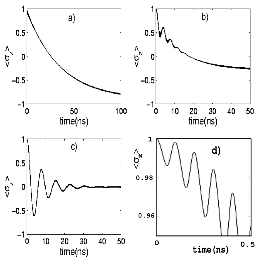
FIG. 1.: $\langle\sigma_{z}\rangle(t)$ at fixed frequency $\Omega/2\pi=6.6$GHz for different bias points. a) Off-resonance, $\nu/2\pi=2.9$GHz, incoherent decay towards thermal equilibrium; c) on-resonance, $\nu/2\pi=6.6$GHz, Rabi oscillations decaying on the scale of a dephasing time $\tau_{\phi}$ towards a dynamical equilibrium state; b) close to the resonance, $\nu/2\pi=6.4$ GHz, combination of decoherence and relaxation; d) short-time dynamics highlighting the fast oscillating component, see text.

We have numerically solved the driven Bloch-Redfield equation. The real-time dynamics is illustrated in fig. 1.

The dynamics shows distinct features on different time scales. As expected, there are clear Rabi oscillations on the scale of the effective driving strength (see below). In quantum computing applications, these would be used for the implementation of a Hadamard gate. On top of this, there are fast components: The dominating one oscillates with the driving frequency, which originates in the fact that the driving is not perpendicular to the static field. A weaker one, which oscillates at twice the driving frequency, comes from the counter-rotating term perpendicular to the static field. These oscillations can lead to errors of the Hadamard gate. On a longer time scale, the Rabi oscillations decay. The time scales will be discussed later on. In general, if one is not exactly on resonance, these oscillations are combined with nonoscillatory decay, see fig. 1 a) and b). At very long times, the system assumes a quasistationary value $P_{\infty}$.

Corresponding to the situation of a spectroscopy experiment, we now turn to the analysis of the quasi-stationary state which is established after a long time $t\gg\tau_{\phi},\tau_{R},\omega_{R}^{-1}$. We compare our full numerical solutions with analytical expressions we have obtained from the high-frequency approximation of Refs. [7, 14]. As a result of this approach, the TSS is mapped onto a coupled ensemble of TSSs corresponding to the original system emitting or absorbing $n$ photons from the driving field during the tunneling. The energy bias of these individual systems is $\epsilon_{n}=\epsilon_{0}-n\Omega$ and the tunnel matrix element

$$\Delta_{n}=\Delta J_{n}(s/\Omega)$$ (2)

where the $J_{n}$ are Bessel functions. At low driving fields, we can approximate $\Delta_{n}=\frac{\Delta}{n!}(s/2\Omega)^{n}$ as we would expect from the expansion of a perturbation series in the driving strength. The $\Delta_{n}$ can hence be viewed as $n$-photon Rabi frequencies. This implies, that the usual single-photon frequency gets replaced by $\Delta_{1}\simeq s\Delta/\nu$, which can be interpreted as only the projection of the driving field onto the direction in pseudospin space orthogonal to the static Hamiltonian. In order to obtain the solid curves in fig. 2 the secular equations for the Eigenfrequencies have been solved, taking into account an appropriate number of terms [16]. The dynamical two state systems are characterized by individual dynamical dephasing rates $\Gamma_{\phi,n}$ and a common relaxation rate $\Gamma_{r}$ [7]. On the n-th resonance, $\Gamma_{\phi,n}$ can be very low, much lower than off-resonance, as can be seen in figure 1, and largely exceed the intrinsic dephasing time. This has been observed in Refs. [1, 4].

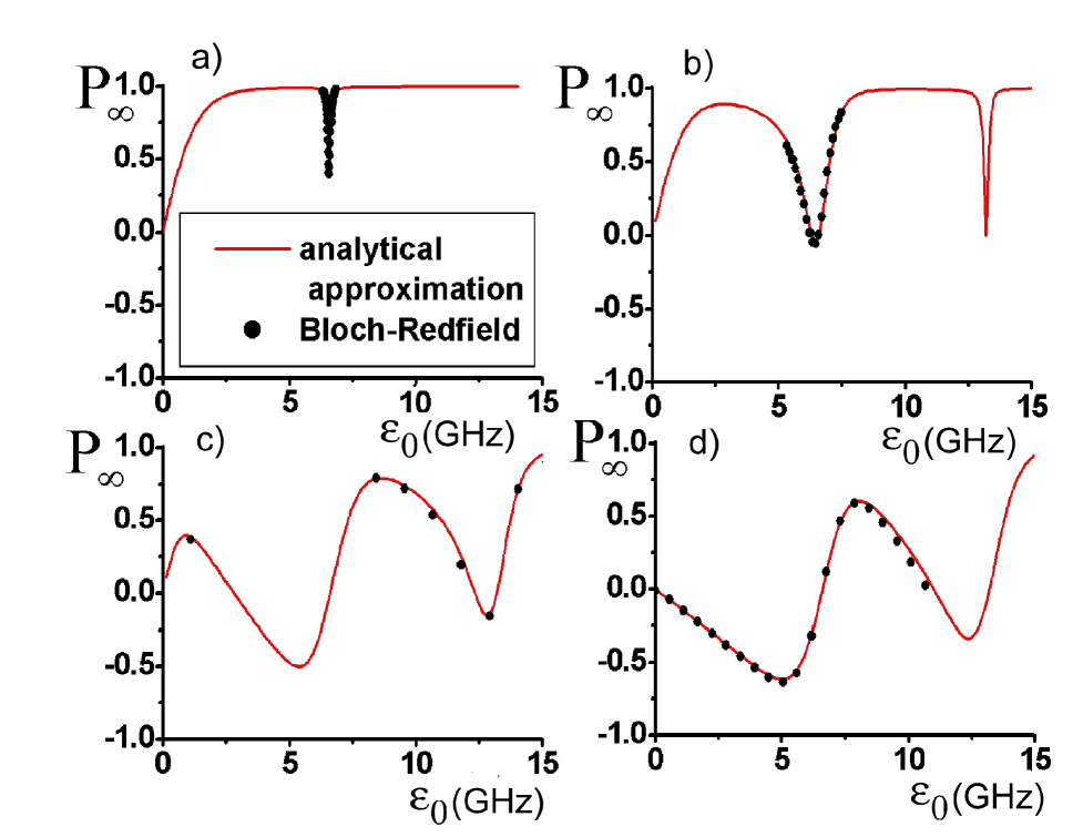
FIG. 2.: $\langle\sigma_{z}\rangle$ in the long-time limit at fixed frequency $\Omega/2\pi=6.6$GHz as a function of the energy bias $\epsilon_{0}$ for different values of the driving strength $s/\Omega=0.034,0.43,1.7,2.4$ (a to d). From b to d, nonlinear resonances can be identified. d already shows negative values at small positive $\epsilon_{0}$, which can be identified as the coherent destruction of zero-photon tunneling. Further peaks occur at even higher bias.

Figure 2 shows numerical and analytical results for $P_{\infty}=\lim_{t\rightarrow\infty}\langle\sigma_{z}\rangle$ at a fixed frequency $\Omega/2\pi=6.6$GHz as a function of the energy bias $\epsilon_{0}$. This corresponds to a realistic experimental situation [3]. In fig. 2 a), taken at weak driving field, only the regular resonance corresponding to the transition between the two Eigenstates driven by absorbing a single photon can be seen. At somewhat stronger driving, fig. 2 b), this peak grows wider and a second resonance appears, corresponding to the simultaneous absorption of two photons. At higher fields, fig. 2 c), these peaks grow and start to dominate over the background. They also turn asymmetric. This trend culminates in the situation shown in fig. 2 d). In that case, $P_{\infty}$ does not grow to positive values at small positive $\epsilon_{0}$, but it gets negative and then directly approaches the first resonance. The reason for this behavior can be identified within the high-frequency approximation: The lowest order-tunnel frequency $\Delta_{0}=\Delta J_{0}(s/\Omega)$ vanishes at this particular driving strength. Indeed, comparing figs. 2 a) and d) one can see, that the step which is at $\epsilon_{0}=0$ in case a) is shifted to $\epsilon_{0}\simeq\Omega$ in case d). This phenomenon, the coherent desctruction of tunneling [6] relies on destructive interference of the dressed state [17] formed by the TSS and a cloud of photons from the driving field. This interpretation is supported by the dynamics of $\langle\sigma_{z}\rangle(t)$. As seen in fig. 3, which shows the dynamics at the degeneracy point for different driving strengths, the zero-photon tunneling is slowed down and brought to a standstill. If that strong driving can be applied to solid-state qubits, it would provide an alternative for controlling $\Delta_{0}$ by a cw microwave field instead of an additional magnetic flux as proposed in Ref. [2].

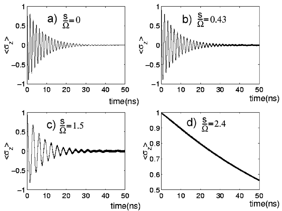
FIG. 3.: $\langle\sigma_{z}\rangle$ at strong driving with high frequency, $\Omega/2\pi=6.6$ GHz (where $\Delta/2\pi=660$ MHz) By increasing the driving strength, the tunneling is slowed down and brought to a standstill.

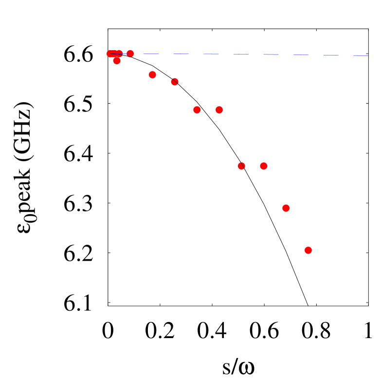
FIG. 4.: Shift of the spectroscopy peak as a function of the driving strength for $\omega/2\pi=6.6$GHz and $\Delta/2\pi$=660 MHz. We compare to the usual Bloch-Siegert shift formula (dashed) and the formula derived in the text (solid).

At very weak driving, the peak position corresponds to the qubit eigenfrequency, $\Omega=\nu$. This is not reliably predicted by the high-frequency approximation. At stronger driving, the peak gets shifted. Closer inspection as in figure 4 shows, that this shift goes much beyond the usual Bloch-Siegert shift [6] of the dynamical Eigenfrequency, in fact, one can show that the position of the peak in steady state and the Eigenfrequency do not conincide. The former is given by balancing of rates and it can be shown that in lowest order gets shifted by[16] $\delta\epsilon_{\rm peak}\simeq s^{2}/8\Omega^{2}$ whereas the Bloch-Siegert shift for our case is $\delta\epsilon_{\rm BS}\simeq\Delta^{2}s^{2}/(16\Omega^{3})$. As a more general conclusion, already at modest not-too-weak driving, the resonance positions do not necessarily reflect the Eigenfrequencies of the system.

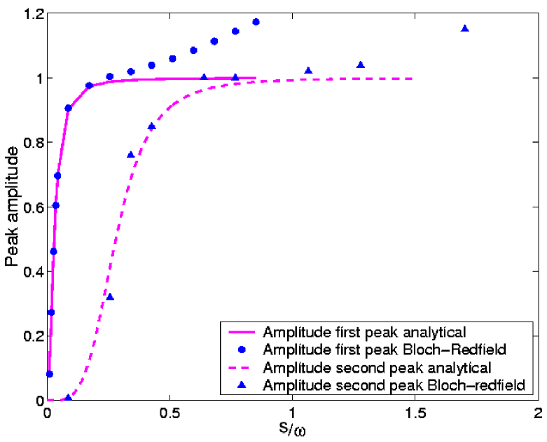
FIG. 5.: Heights of the two lowest resonances as a function of the driving strength $s$ at $\nu/2\pi=6.6$ GHz, $\Delta/2\pi=660$ MHz, $\Omega/2\pi=6.6$ GHz The solid and dashed lines are extrapolated NMR formulae.

In fig. 5, the height of the two lowest order peaks is shown. It can be seen, that, from the low-driving side, they saturate as soon as their effective Rabi frequency $\Delta_{n}$ exceeds $1/\sqrt{T_{r}T_{\phi}}$. At very high driving, the peaks show an inversion of population.

For the optimization of qubit setups on the way to coherent dynamics, it is important to characterize its coherence properties from the spectroscopic data. In NMR, this is done from the linewidth given by

$$\delta\Omega=2\sqrt{\tau_{\phi}^{-2}+\omega_{R}^{2}\tau_{R}/\tau_{\phi}}$$ (3)

where $\omega_{R}$ is the Rabi frequency at resonance, which coincides with the strength of the driving field. A generalization of this formula to our case has to take into account low temperatures and the different driving situation. Moreover, $\omega_{R}$ is usually not directly known to sufficient precision, because the driving strength depends on the attenuation of the applied fields on their way to the sample and the efficiency of the coupling [3, 5].

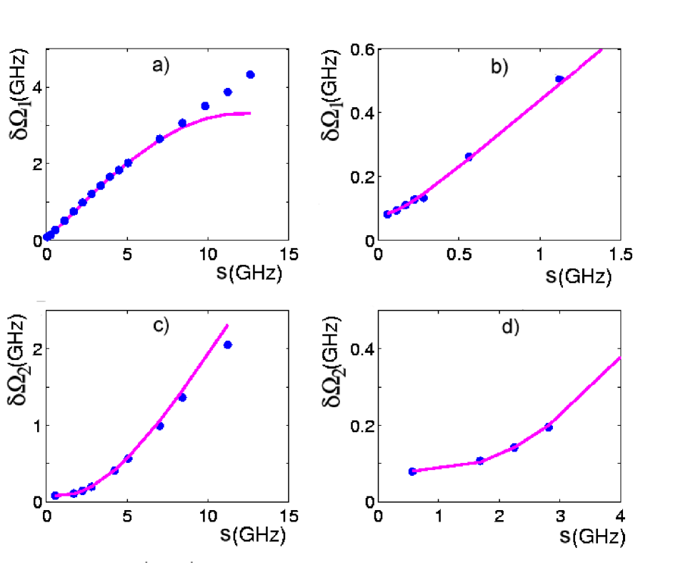
FIG. 6.: Widths of the two lowest resonances as a function of the driving strength $s$ at $\Delta/2\pi=660$ MHz $\Omega/2\pi=6.6$ GHz. The solid line corresponds to the extrapolated NMR formula discussed in the text.

Our analysis suggests the generalization of eq. 3 is given by

$$\delta\Omega_{n}=2\sqrt{\tau_{\phi}^{-2}+\Delta_{n}^{2}\tau_{R}/\tau_{\phi}}\quad n=\pm 1,\pm 2\dots$$ (4)

where $\delta\Omega_{n}$ is the width (in frequency) of the $n$-photon resonance and $\Delta_{n}$ is the effective Rabi frequency defined above. At low powers $s<\Omega$, they are given by the rates from the undriven ohmic case

$$\tau_{\rm R}^{-1}=\alpha\frac{\Delta^{2}}{2\nu}\coth\left(\frac{\hbar\nu}{2k_{B}T}\right)\quad\tau_{\rm\phi}^{-1}=(2\tau_{R})^{-1}+2\pi\alpha\frac{k_{B}T}{\hbar}\frac{\epsilon_{0}^{2}}{\nu^{2}}.$$ (5)

This result is confirmed by our numerical simulations fig.  6. We can essentially identify three regimes: A saturation broadening regime at low powers, where $\delta\Omega_{n}\simeq 2\tau_{\rm\phi}^{-1}$, a saturated regime, $\delta\Omega_{n}\simeq 2\Delta_{n}\sqrt{\tau_{R}/\tau_{\phi}}$ and a nonlinear regime, where the numerical curve deviates from eq. 4 due to the fact, that the high Rabi frequency shifts the relevant energy scales and modifies the timescales given in eq. 5. Note, that in this regime, the general curve of $P_{\infty}$ is greatly deformed (see fig. 2) and the width of a peak becomes ambiguous.

This result allows to measure essentially all interesting parameters of the system experimentally. By extrapolating the level separation at the degeneracy point (as it was done in [3]), one obtains $\Delta$. By tracking the resonance positions at weak driving, one can evaluate $\epsilon_{0}$ as a function of the external control parameter (in [3] this would be the magnetic flux). By driving in the saturated regime, the widths of the first and second peak become, according to eq. 4 $\delta\Omega_{1/2}=2\Delta_{1/2}\sqrt{\tau_{R}/\tau_{\phi}}$, hence by taking their ratio we find the effective driving strength from $\Delta_{2}/\Delta_{1}=J_{1}(s/\Omega)/J_{0}(s/\Omega)\simeq s/2$ and by tracking the slope of the first resonance we find the ratio $\tau_{r}/\tau_{\phi}$. Finally, examining the saturation broadening regime of the first resonance gives the absolute value of $\tau_{\phi}$.

In conclusion, we have numerically and analytically analyzed the spin-boson system, which e.g. represents a SQUID-qubit, in the weak damping regime, driven by continuous fields. As compared to the more familiar situation in NMR, this system is both different in the character of the driving and the low temperature governing the dissipation. We have shown, that the key features of this system, Rabi-oscillations, and saturation of the linewidth, persist qualitatively as has been experimentally confirmed [4]. They are however altered on a quantitative level, such as an unanticipatedly strong shift of the position of the resonance peak, and also supplemented by new phenomena such as higher-harmonics generation, oscillations of $\langle\sigma_{z}\rangle$ on the scale of the driving field, and coherent desctruction of tunneling. We have finally outlined a scheme how to determine all relevant parameters (tunnel splitting, energy dispersion, driving strength, dephasing and relaxation time) of a quantum bit solely through spectroscopy.

We thank M. Grifoni, C.H. van der Wal, A.C.J. ter Haar, C.J.P.M. Harmans, J. von Delft and I. Goychuk for discussions. Work supported by the EU through TMR “Supnan” and IST “Squbit”. FKW acknowledges support by the ARO under contract-Nr. P-43385-PH-QC.

REFERENCES

- [1] D. Vion et al., Science 296, 886 (2002).
- [2] J.E. Mooij et al., Science 285, 1036 (1999).
- [3] C.H. van der Wal et al., Science 290, 773 (2000).
- [4] I. Chiorescu, Y. Nakamura, C.J.P.M. Harmans, and J.E. Mooij, Science 299, 1869 (2003).
- [5] C.H. van der Wal et al., Eur. Phys. J. B 31, 111 (2003). T.P. Orlando et al., Physica C 368, 294 (2002).
- [6] P. Hänggi and M. Grifoni, Phys. Rep. 304, 229 (1998).
- [7] L. Hartmann at al., Phys. Rev. E 61, 4687 (2000).
- [8] A.J. Leggett et al., Rev. Mod. Phys. 59, 1 (1987).
- [9] U. Weiss, Quantum Dissipatice Systems, 2nd ed., (World Scientific, Singapore, 1999).
- [10] A.C.J. ter Haar et al., private communication.
- [11] A. Wallraff et al., cond-mat/0206227.
- [12] Y. Nakamura, Yu.A. Pashkin, and J.S. Tsai, Phys. Rev. Lett. 87, 246601 (2001).
- [13] P.N. Argyres and P.L. Kelley, Phys. Rev. 134, A98 (1964).
- [14] M. Grifoni, M. Sassetti, and U. Weiss, Phys. Rev. E 53, R2033 (1996).
- [15] A. Abragam, The principles of Nuclear magnetism (Oxford University Press, Glasgow, 1961).
- [16] for details see M.C. Goorden, Master’s thesis, TU Delft (2002); available on qt.tn.tudelft.nl
- [17] M. Thorwart, L. Hartmann, I. Goychuk, and P. Hänggi, J. Mod. Opt. 47, 2905 (2000).