slow switching in a population of delayed pulse-coupled oscillators

Abstract

We show that peculiar collective dynamics called slow switching arises in a population of leaky integrate-and-fire oscillators with delayed, all-to-all pulse-couplings. By considering the stability of cluster states and symmetry possessed by our model, we argue that saddle connections between a pair of the two-cluster states are formed under general conditions. Slow switching appears as a result of the system’s approach to the saddle connections. It is also argued that such saddle connections easy to arise near the bifurcation point where the state of perfect synchrony loses stability. We develop an asymptotic theory to reduce the model into a simpler form, with which an analytical study of cluster states becomes possible.

I introduction

Studies on collective motion of coupled oscillators have attracted considerable attention over the last few decadeswinfree67 ; kuramoto84 ; synchronization . It is commonly seen that a population of autonomous elements performs certain biological functions by behaving collectivelyfromneuron . It has in fact been pointed out that collective motion is crucial to information processing and transmission in living organismsbinding .

In the brain, the neurons are exclusively coupled through chemical synapses, i.e., the neurons communicate by pulses of transmittermethods . Chemical synapses commonly form dense and complex networks. For mathematical modeling of neuronal networks, homogeneous all-to-all (or, global) coupling is often adopted. Although the global coupling may be a little too idealistic, the corresponding networks share a lot of properties in common with systems with complex and dense networks.

In the present paper, we consider a population of neural oscillators with delayed, all-to-all pulse-coupling. The oscillator we use is called the leaky integrate-and-fire (LIF) model. There are a large amount of papers concerning LIF in physics and neuroscience, e.g., see mirollo90 ; kuramoto91 ; sakai99 . This is because LIF is a quite simple model still capturing some essential characteristics of neuronal dynamics, i.e., it represents an integrator with relaxation, and resets after it fires. Though our population model is commonly used, (e.g., see abbott93 ), its collective dynamics does not seem to have been studied so carefully. We are particularly concerned with peculiar collective dynamics called slow switchinghansel93 ; kori01 . The study of collective dynamics in the original form of the model is not easy to handle because the coupling involves a long term memory. We thus develop an asymptotic theory and reduce our model into a form without memory, by which an analytical study of collective dynamics becomes possible.

II model

The population model we consider consists of $N$ identical elements with delayed, all-to-all pulse-coupling. The dynamics of each elements is described by a single variable $v_{i}$ ($i=1,2,\ldots,N$) which corresponds to the membrane potential of a neuron. The equation for $v_{i}$ is given by

$$\frac{d}{dt}v_{i}(t)=a-v_{i}+\frac{K}{N}(b-v_{i})E(t).$$ (1)

The parameter $a$ is the so-called resting potential to which $v_{i}$ relaxes when the coupling is absent. It is assumed that when $v_{i}$ reaches a threshold value which is set to $1$, it is instantaneously reset to zero. This event is interpreted as a spiking event. The dynamics is thus called LIF. When a neuron spikes, it emits a pulse toward each neuron coupled to it, and the latter receives the pulse with some delay called a synaptic delay. The coupling is assumed to be homogeneous and all-to-all, so that its effect can be represented by one global variable $E$, given by

$$E(t)=\sum_{j=1}^{N}\sum_{\rm spikes}e(t-t_{j}^{\rm spikes}-\tau).$$ (2)

Here, ${t_{j}^{\rm spikes}}$ represents a series of times at which the $j$-th neuron spikes and $\sum_{\rm spikes}$ denotes a summation over the series of such spikes; $\tau$ is the synaptic delay, and $e(t)$ is a pulse function, given by

$$e(t)=\frac{\alpha\beta}{\beta-\alpha}(e^{-\alpha t}-e^{-\beta t})\Theta(t),$$ (3)

where $\Theta(t)$ is the Heaviside function; $\alpha$ and $\beta$ are constants satisfying $\beta>\alpha$. In the limit $\beta\to\alpha$, $e(t)$ becomes $\alpha^{2}te^{-\alpha t}$, which is called the alpha functionmethods . $b$ is called the reversal potential to which $v_{i}$ relaxes when $E(t)$ is positive, i.e., while the neuron receives the pulses. $K$ is a positive constant characterizing the strength of the coupling. The coupling assumed above is characteristic to the synaptic coupling. The coupling become excitatory (EPSP) if $b>1$, and inhibitory (IPSP) if $b\leq 0$.

If $a\leq 1$, LIF becomes an excitable neuron, while if $a>1$, it repeats periodic spikes, namely, it represents a neural oscillator. We assume $a>1$ throughout the present paper, and call each element an oscillator. Then, we can define a variable $\psi_{i}$ varying smoothly with time, which turns out useful in the following discussion. We call $\psi_{i}$ the phase of the $i$-th oscillator, and define it by

$$\psi_{i}=\int_{0}^{v_{i}}\frac{dv}{a-v}=\ln\left(\frac{a}{a-v_{i}}\right),$$ (4)

which varies between $0$ and the intrinsic period of oscillation $T$ given by

$$T=\ln\left(\frac{a}{a-1}\right).$$ (5)

Note that $\psi_{i}$ satisfies $d\psi_{i}/dt=1$ in the absence of coupling.

III numerical results

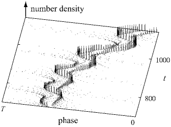
Figure 1: Slow switching phenomenon viewed through the number density of the oscillators as a function of phase. In order to get a better view, we work with a comoving frame of reference. The parameter values are $a=1.03$ ($T\simeq 3.5$), $b=2.0,\alpha^{-1}=0.3,\beta\to\alpha,\tau=0.2,K=0.1$ and $N=100$.

By numerically integrating our model under random initial distributions of $v_{i}$, we find various types of collective behavior. Among them, we are particularly interested in the slow switching phenomenon, which can arise when $b>a$ and $N\geq 4$. As displayed in Fig. 1, the whole population, which was initially distributed almost uniformly, splits into two subpopulations, each of which converges almost to a point cluster. However, after some time the phase-advanced cluster starts to scatter. Then, this scattered group starts to converge again as it comes behind the preexisting cluster. In this way, the preexisting cluster becomes a phase-advanced cluster. After some time, again, this phase-advanced cluster begins to scatter, and a similar process repeats again and again. In other words, the system switches back and forth between a pair of two-cluster states. For larger times, the system comes closer to each of well-defined two-cluster states and stays near the state longer. Theoretically, these switchings repeats indefinitely, although in numerical integrations the system converges at one of the two-cluster states in a finite time and stops switching due to numerical round-off errorskori01 .

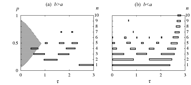
Figure 7: Phase diagrams of cluster states, where $\tau$ is chosen as a control parameter. The parameter values are the same as in Fig. 2 with (a)$b>a$ and (b)$b<a$, respectively. For given $p$ and $\tau$ inside the gray region, $\gamma$ is larger than one, i.e., the heteroclinic loop between $(p,\Delta)$ and $(p,-\Delta^{\prime})$ is attracting. Each rectangle placed at $n$ indicates the region of $\tau$ within which the symmetric $n$-cluster state is stable. In (b), stable symmetric $n$-cluster states with $n>10$ also exist (not shown).

The slow switching phenomenon occurs within a broad range of parameter values provided that $K$ is small, and the time constants $\alpha^{-1},\beta^{-1}$ and $\tau$ are small compared with $T$. For larger $\alpha^{-1},\beta^{-1}$ and $\tau$, the slow switching phenomenon becomes less probable, and the appearance of steady multi-cluster states becomes more probable instead. For $b<a$, we find no two-cluster states involving slow switching, while steady multi-cluster states are observed in most cases. The corresponding phase diagram will be presented in Sec. VII (see Fig. 7).

IV weak coupling limit

Our model given by Eq. (1) is relatively simple, still it would be difficult to get some insight into its collective dynamics analytically. Fortunately, however, our main results given in Sec. III do not change qualitatively in the weak coupling limit, i.e., $K\to 0$. In this limit, our model is reduced to a much simpler form with which we can study the existence and stability of various cluster states analytically. Derivation of the reduced model is given as follows.

Substituting $v_{i}=a(1-e^{-\psi_{i}})$ into Eq. (1), we obtain

$$\frac{d}{dt}\psi_{i}(t)=1+\frac{K}{N}\sum_{j=1}^{N}\sum_{\rm spikes}Z(\psi_{i})e(t-t_{j}^{\rm spikes}-\tau),$$ (6)

where

$$Z(\psi_{i})=\frac{b-a}{a}e^{\psi_{i}}+1.$$ (7)

It is convenient in the following calculation to redefine $Z$ as a $T$-periodic function, or, $Z(\psi_{i}+nT)=Z(\psi_{i})$ ($n=\pm 1,\pm 2,\cdots$). Note that sudden drop of $Z(x)$ at $x=0$ is due to our rule employed, i.e., the membrane potential is instantaneously reset at $v_{i}=1$. We also define a residual phase $\Psi_{i}$ by

$$\Psi_{i}=\psi_{i}-t.$$ (8)

Substituting Eq. (8) into Eq. (6), we obtain

$$\frac{d}{dt}\Psi_{i}(t)=\frac{K}{N}\sum_{j=1}^{N}\sum_{\rm spikes}Z(\Psi_{i}+t)e(t-t_{j}^{\rm spikes}-\tau).$$ (9)

We now assume that $K$ is sufficiently small so that the r.h.s of Eq. (9) is sufficiently smaller than the intrinsic frequency $T^{-1}$. This allow us to make averaging of the r.h.s of Eq. (9) over the period $T$. The zeroth order approximation with respect to the smallness of $K$, which corresponds to the free oscillations, is given by

$$\Psi_{i}(t)=\rm const.$$ (10)

and

$$t_{j}^{\rm spikes}=t_{j}-nT,\quad(n=0,1,2,\ldots),$$ (11)

where $t_{j}$ is the latest time at which the $j$-th neuron spikes. In the first order approximation, we may time-average Eq. (9) over the range between $t-T$ and $t$ using Eqs. (10) and (11):

$$\frac{d}{dt}\Psi_{i}(t) = \frac{K}{N}\sum_{j=1}^{N}\frac{1}{T}\int_{t-T}^{t}\sum_{n=0}^{\infty}Z(\Psi_{i}(t)+\lambda)e(\lambda-t_{j}+nT-\tau)d\lambda$$ (12)

$$= \frac{K}{N}\sum_{j=1}^{N}\frac{1}{T}\int_{0}^{\infty}Z(\Psi_{i}(t)+t_{j}+\tau+\lambda^{\prime})e(\lambda^{\prime})d\lambda^{\prime}$$ (13)

$$= \frac{K}{T}+\frac{K(b-a)}{Na}\sum_{j=1}^{N}\Gamma\bigr{(}\Psi_{i}(t)+t_{j}+\tau\bigl{)},$$ (14)

where

$$\Gamma(x)=\frac{\alpha\beta}{\beta-\alpha}\bigl{\{}H_{\alpha,T}(x)-H_{\beta,T}(x)\bigr{\}},$$ (15)

$$H_{\alpha,T}(x) = \frac{1}{T}\int_{0}^{\infty}\exp[{(x+\lambda)\ {\rm mod}\ T}]\exp[{-\alpha\lambda}]d\lambda$$ (16)

$$= \frac{(e^{T}-1)\exp[{\alpha(x\ {\rm mod}\ T)}]-(e^{\alpha T}-1)\exp[{x\ {\rm mod}\ T}]}{T(1-\alpha)(e^{\alpha T}-1)}.$$

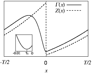
Figure 2: The solid line shows the coupling function $\Gamma(x)$ for $a=1.05$ ($T\simeq 3.0$), $\alpha^{-1}=0.2$ and $\beta\to\alpha$. The minimum appears at $x=\tau_{c}$ which is a small negative. For comparison, the shape of $Z(x)$ is also displayed with the broken line.

Note that $\Gamma(x)$ and $H_{\alpha,T}(x)$ are $T$-periodic functions. Figure 2 illustrates a typical shape of the coupling function given by Eq. (15). Furthermore, using the identity

$$\Psi_{j}(t_{j})=\psi_{j}(t_{j})-t_{j}=-t_{j},$$ (17)

and the zeroth order approximation $\Psi_{j}(t_{j})=\Psi_{j}(t)$, we may replace $t_{j}$ by $-\Psi_{j}(t)$ in Eq. (14) in the first order approximation. Thus, we finally obtain

$$\frac{d}{dt}\psi_{i}(t)=\omega+\frac{K^{\prime}}{N}\sum_{j=1}^{N}\Gamma\bigr{(}\psi_{i}(t)-\psi_{j}(t)+\tau\bigl{)},$$ (18)

where $\omega=1+K/T$ and $K^{\prime}=K(b-a)/a$. Equation (18) is the standard form of the phase model. Note that the error involved in Eq. (11) may look to diverge as $n\to\infty$, still the final error vanishes in the first order approximation due to the decay of $e(t)$. It should be noted that the reduced model is free from memory effects, but the effect of delay has been converted to a phase shift in the coupling function. Similar form of the phase model is generally obtained in delayed coupled oscillators when the coupling is sufficiently weakkori01 . Hereafter, we ignore the degree of freedom associated with the dynamics of the center of mass (or, mean phase) which can be decoupled in the phase model.

Important parameters of our phase model given by Eq. (18) with Eq. (15) are $T,\alpha,\beta,\tau$ and the sign of $K^{\prime}$ (i.e., the sign of $b-a$). The reason is the following. We may take $|K^{\prime}|=1$ by properly rescaling of $t$ and $\omega$, while its sign is crucial because the local stability of any solution depends on it. $\omega$ gives the frequency of steady rotation of the whole system, which is irrelevant to collective dynamics. We choose $T$ as an independent parameter by which $a$ becomes dependent through Eq. (5). It is remarkable that our coupling function is independent of $b$. In fact, change in $b$ causes no qualitative change in our result as far as the sign of $b-a$ remains the same. Interestingly, even if we replace the term $b-v_{i}$ by a constant $c$ in Eq. (1), i.e.,

$$\frac{d}{dt}v_{i}(t)=a-v_{i}+\frac{Kc}{N}E(t),$$ (19)

then we can reduce this model similarly and obtain the same coupling function as in Eq.(15). We have checked that Eq. (19) actually reproduces qualitatively the same results as those given in Sec. III. In that case, negative $c$ corresponds to the case $b<a$ in Eq. (1).

In the following section, we assume $b>a$ and $\beta\to\alpha$ unless stated otherwise.

V two-oscillator system

In this section, we study a two-oscillator system, or, $N=2$. Although the two-oscillator system is not directly related to the main subject of the present paper, one may learn some basic properties of our phase model from this simple case. Defining $\Delta=\psi_{1}-\psi_{2}$, we obtain

$$\frac{d\Delta}{dt}=\frac{K^{\prime}}{2}\bigl{(}\Gamma(\Delta+\tau)-\Gamma(-\Delta+\tau)\bigr{)}\equiv G_{\tau}(\Delta).$$ (20)

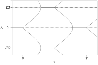
Figure 3: Bifurcation diagram of a two-oscillator system. Solid and dotted lines respectively represent stable and unstable branches, where $b>a$ is assumed. The stability property is reversed if $b<a$.

Phase locking solutions are obtained by putting $d\Delta/dt=0$, and the associated eigenvalues are given by $dG_{\tau}/d\Delta$. Figure 3 shows a bifurcation diagram of the phase locking solutions, in which we take $\tau$ as a control parameter. We find that for small $\tau$ the trivial solutions $\Delta=0$ (in-phase locking) and $T/2$ (anti-phase locking) are unstable, while there are a pair of stable branches of non-trivial solutions. The point $\tau=0$ is close to the bifurcation point where the in-phase state loses stability. The bifurcation occurs at $\tau=\tau_{\rm c}$, where $\tau_{\rm c}$ corresponds to the minimum of $\Gamma(x)$ (see Fig. 2). Because $\tau_{\rm c}$ is negative, the in-phase state cannot be stable for small or vanishing delays (while it can be stable for delays comparable to $T$ due to the $T$-periodic nature of our phase model). $\tau_{\rm c}$ is extremely small, which is due to the sudden drop of $Z(x)$ at $x=0$ and the particular rule employed in our model, i.e., a neuron is assumed to spike and reset simultaneously. The width of the stable branches of the trivial solutions is the same as that of the decreasing part of $\Gamma(x)$. Owing to the peculiar shape of $Z(x)$, the width is of the same order as the width of $e(t)$, which is $O(\alpha^{-1})$. The stability of the in-phase state is identical with that of the state of perfect synchrony.

In terms of the original model, we now present a qualitative interpretation of why the in-phase locking state is unstable for small or vanishing delays. We consider the dynamics of two neurons which are initially very close in phase. The effect of a pulse on the phase $\psi_{i}$ is larger for smaller $dv_{i}/dt$. $dv_{i}/dt$ is monotonously decreasing except when it is reset (which reflects on the property of $Z(x)$ that it is increasing except $x=0$). Thus, the neuron with larger $v_{i}$ makes a larger jump in phase when it receives a pulse, by which the phase difference between the two neurons becomes larger when they receive a pulse. On the other hand, the situation becomes different if two neurons lie before and after the resetting point, i.e., if the phase-advanced neuron has smaller $v_{i}$. In that case, the phase difference becomes smaller when they receive a pulse. According to our dynamical rule, however, resetting and spiking occur simultaneously, so that they receive pulses when the phase-advanced neuron has larger $v_{i}$. Therefore, the in-phase state becomes inevitably unstable even without delay. If we want to obtain a stable in-phase state for small delays, we should employ a rule such that a neuron spikes before it is reset, which would be more physiologically plausible than the rule employed here.

VI local stability analysis for a large population

The trivial in-phase solution and the non-trivial solutions of the two-oscillator system correspond respectively to the state of perfect synchrony and two-cluster states when we go over to a large population. In this section, we study local stability of the two-cluster states. Although non-trivial solutions are stable for small or vanishing delays in the two-oscillator system, the corresponding two-cluster states turn out unstable.

We consider a steadily oscillating two-cluster state in which the two clusters consist of $Np$ and $N(1-p)$ oscillators, respectively. The oscillators inside each cluster are completely phase-synchronized, and the phase-difference between the clusters is constant in time, which is denoted by $\Delta$. From Eq. (18), the phase difference obeys the equation

$$\frac{d\Delta}{dt}=K^{\prime}\left\{(2p-1)\Gamma(\tau)+(1-p)\Gamma(\Delta+\tau)+p\Gamma(-\Delta+\tau)\right\}.$$ (21)

When $\Delta$ is constant, we obtain a relation between $p$ and $\Delta$ as

$$(2p-1)\Gamma(\tau)+(1-p)\Gamma(\Delta+\tau)+p\Gamma(-\Delta+\tau)=0.$$ (22)

We designate a two-cluster state satisfying Eq. (22) as $(p,\Delta)$. The eigenvalues of the stability matrix are calculated as

$$\lambda_{1}=K^{\prime}\{p\Gamma^{\prime}(\tau)+(1-p)\Gamma^{\prime}(\Delta+\tau)\},$$ (23)

$$\lambda_{2}=K^{\prime}\{(1-p)\Gamma^{\prime}(\tau)+p\Gamma^{\prime}(-\Delta+\tau)\},$$ (24)

$$\lambda_{3}=K^{\prime}\{(1-p)\Gamma^{\prime}(\Delta+\tau)+p\Gamma^{\prime}(-\Delta+\tau)\},$$ (25)

where $\Gamma^{\prime}(x)$ means $(d/dx)\Gamma(x)$. The multiplicities of $\lambda_{1},\lambda_{2}$ and $\lambda_{3}$ are $Np-1$,$N(1-p)-1$ and $1$, respectively. $\lambda_{1}$ and $\lambda_{2}$ correspond to fluctuations in phase of the two oscillators inside the phase-advanced and phase-retarded cluster, respectively. $\lambda_{3}$ corresponds to fluctuations in the phase difference $\Delta$ between the clusters.

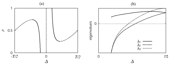
Figure 4: (a)Relation between $p$ and $\Delta$ associated with two-cluster states. (b)Eigenvalues of two-cluster states as a function of $\Delta$. In (a), the solid and dotted lines correspond to the two-cluster state of negative and positive $\lambda_{3}$, respectively.

Substituting Eq. (15) into Eq. (22), we obtain a relation between $p$ and $\Delta$, the corresponding curve being shown in Fig. 4(a). By using this relation, the eigenvalues of $(p,\Delta)$ can be obtained, which are displayed in Fig. 4(b) as a function of $\Delta$. It is found that no two-cluster states are stable, and there is a set of $(p,\Delta)$ for which $\lambda_{1}>0$ and $\lambda_{2},\lambda_{3}<0$. Positive $\lambda_{1}$ means that the two-cluster state is unstable with respect to perturbations inside a phase-advanced cluster. On the other hand, $\lambda_{2},\lambda_{3}<0$ means that it is stable against perturbations inside a phase-retarded cluster as far as the perfect phase-synchrony of the phase-advanced cluster is maintained. Within a certain range of $p$, there are pairs of two-cluster states represented by $(p,\Delta)$ and $(p,\Delta^{\prime})$ with the same stability property, and they appear as the solid lines in Fig 4(a). In the next section, we explain how a heteroclinic loop between the $(p,\Delta)$ and $(p,\Delta^{\prime})$ is stably formed in our model.

Similarly to the discussion in Sec. V, the stability property mentioned above can also be understood in terms of the original model. Every neuron inside the phase-advanced cluster always receives pulses when its membrane potential is increasing. Then, the phase-difference between two neurons inside the cluster, if any, always increases, so that the phase-advanced cluster is inevitably unstable. On the other hand, the neurons inside the phase-retarded cluster can receive pulses (emitted by the phase-advanced cluster) during their resetting. Then, the phase-differences between neurons inside the phase-retarded cluster, if any, become smaller, so that the phase-retarded cluster can be stable.

VII heteroclinic loop

We first note that there is a particular symmetry of our model which turns out crucial to the persistent formation of the heteroclinic loop. The symmetry is given by

$$\left.\frac{d}{dt}\{v_{i}(t)-v_{j}(t)\}\right|_{v_{i}(t)=v_{j}(t)}=0\quad\mbox{for any $i$ and $j$}.$$ (26)

Due to this symmetry, the units which have the same membrane potential at a given time behave identically thereafter. In other words, once a point cluster is formed, it remain a point cluster forever.

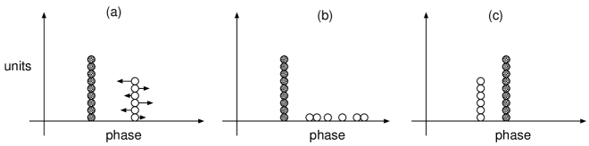
Figure 5: Schematic representation of a saddle connection between a pair of two cluster states, starting with the two-cluster state A (a) ending up with the other two-cluster state B (c).

We assume that a pair of two-cluster states (called A and B) exists and has the same stability property as that discussed in Sec. VI, i.e., the phase-advanced cluster is unstable, and the phase-retarded clusters is stable. Suppose that our system is in a two-cluster state A initially. When the oscillators inside the phase-advanced cluster are perturbed while the phase-retarded cluster is kept unperturbed [see Fig. 5(a)], the former begins to disintegrate while the latter remains a point cluster. Then, the group of dispersed oscillators and the point cluster coexist in the system [see Fig. 5(b)]. We know, however, that in the presence of a point cluster, there exists a stable two-cluster state in which the existing point cluster is phase-advanced. From this fact, the dispersed oscillators are expected to converge to form a point cluster coming behind the preexisting point cluster. In this way, the system relaxes to another two-cluster state B [see Fig. 5(c)]. From the above statement, it is implied that in our high-dimensional phase space there exists a saddle connection from the state A to the state B. The existence of a saddle connection from the state B to the state A can be argued similarly. A heteroclinic loop is thus formed between the pair of the two cluster states A and B.

In terms of the phase model, the above argument can be reinterpreted in a little more precise language. In the phase model given by Eq. (18), a symmetry property similar to Eq. (26) also holds:

$$\left.\frac{d}{dt}\{\psi_{i}(t)-\psi_{j}(t)\}\right|_{\psi_{i}(t)=\psi_{j}(t)}=0\quad\mbox{for any $i$ and $j$}.$$ (27)

Our argument will be based on the following assumptions:

• $(p,\Delta)$ with $\lambda_{1}>0$ and $\lambda_{2},\lambda_{3}<0$ exits,

• $(p,\Delta^{\prime})$ with $\lambda^{\prime}_{2}>0$ and $\lambda^{\prime}_{1},\lambda^{\prime}_{3}<0$ exits,

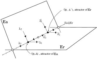
Figure 6: Schematic representation of the structure of a heteroclinic loop. $(p,\Delta)$ and $(p,\Delta^{\prime})$ become attractors in the invariant subspaces $E_{a}$ and $E_{r}$, respectively.

where we define $\Delta>0$ and $\Delta^{\prime}<0$, and $\lambda_{i}$ and $\lambda^{\prime}_{i}$ ($i=1,2,3$) are the eigenvalues of $(p,\Delta)$ and $(p,\Delta^{\prime})$, respectively. Note that if $p=0.5$, the two clusters in question are identical, or $\Delta^{\prime}=\Delta$, so that (a) and (b) are identical. Figure 6 illustrates a schematic presentation of the $N-1$ dimensional phase space structure, where we ignore the degree of freedom associated with the dynamics of the center of mass. $E_{a}$ and $E_{r}$ are identical with the subspaces where the phase-advance and phase-retarded clusters of $(p,\Delta)$ remain point clusters, respectively. By considering the direction of eigenvectors, one can easily confirm that $E_{a}$ and $E_{r}$ are identical with the stable subspaces of $(p,\Delta)$ and $(p,\Delta^{\prime})$, respectively. Furthermore, because $E_{a}$ and $E_{r}$ are invariant subspaces due to the symmetry given by Eq. (27), $(p,\Delta)$ and $(p,\Delta^{\prime})$ are attractors within $E_{a}$ and $E_{r}$, respectively. Thus, a heteroclinic loop between $(p,\Delta)$ and $(p,\Delta^{\prime})$ should necessarily exits. The saddle connections in question are stably formed through the invariant subspaces which exist for the symmetry of equations of motion given by Eq. (27). The heteroclinic loop is thus robust against small perturbations to the system unless the symmetry is broken.

Whether the resulting heteroclinic loop is attracting or not depends on the following quantity:

$$\gamma\equiv\frac{\lambda_{2}\lambda^{\prime}_{1}}{\lambda_{1}\lambda^{\prime}_{2}}.$$ (28)

It was argued in Ref. hansel93 that if $\gamma>1$, the system can approach the heteroclinic loop and come to move along it. In that case, the time interval during which the system is trapped to in the vicinity of one of the two-cluster states increases exponentially with time. Substituting the eigenvalues obtained from Eqs. (23) and (24) using Eq. (15) into Eq. (28), we find that the heteroclinic loops within a certain range of $p$ are in fact attracting for small $\alpha^{-1},\beta^{-1}$ and $\tau$. Phase diagrams of the heteroclinic loops and symmetric multi-cluster states is shown in Fig. 7, where we choose $\tau$ as a control parameter (see appendix for the stability of the symmetric multi-cluster states).

VIII near the bifurcation point

In this section, we concentrate on the vicinity of the bifurcation point where the state of perfect synchrony loses stability. As noted in Sec. V, the bifurcation occurs at $\tau=\tau_{\rm c}$. Then, for small $x-\tau_{\rm c}$, the coupling function can be expanded as

$$\Gamma(x)=c_{0}+c_{2}(x-\tau_{\rm c})^{2}-c_{3}(x-\tau_{\rm c})^{3}+O((x-\tau_{\rm c})^{4}).$$ (29)

Suppose that $c_{2}$ and $c_{3}$ are positive. We further put $c_{3}=1$ by properly rescaling $K^{\prime}$ in Eq. (18). In order to find possible two-cluster states, we solve Eq. (22) using Eq. (29). We then obtain three solutions for $\Delta$ as a function of $p$ and $\tau$. One is the trivial solution $\Delta=0$ (the perfect synchrony), and the others are given by

$$\Delta=\frac{(1-2p)(c_{2}-3\tilde{\tau})}{2}\pm\sqrt{\frac{(1-2p)^{2}(c_{2}-3\tilde{\tau})^{2}}{4}+2c_{2}\tilde{\tau}},$$ (30)

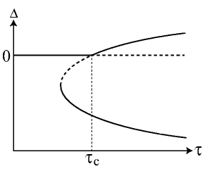
Figure 8: Bifurcation diagram around $\tau=\tau_{c}$. A heteroclinic loop is formed between a pair of the solid branches for $\tau>\tau_{c}$.

where $\tilde{\tau}\equiv\tau-\tau_{\rm c}$. Note that the expression above using the approximate $\Gamma$ given by Eq. (29) is valid only for small $\Delta$, which is actually the case if $p$ is close to $1/2$ and $\tilde{\tau}$ is small. Substituting the expressions in Eq. (30) into Eqs. (23)-(25), we obtain eigenvalues associated with the two-cluster states. The resulting bifurcation diagram for given $p$ is shown in Fig. 8. The solid and broken lines give the branches of negative and positive $\lambda_{3}$, respectively. Two solid branches exist for $\tau>0$, which are represented by $(p,\Delta)$ and $(p,\Delta^{\prime})$ with $\Delta>0$ and $\Delta^{\prime}<0$. One can easily confirm that the eigenvalues of these states satisfy $\lambda_{1},\lambda^{\prime}_{2}>0$ and $\lambda_{2},\lambda_{3},\lambda^{\prime}_{1},\lambda^{\prime}_{3}<0$ for arbitrary $p$ and small $\tilde{\tau}$, which agree with the condition for the existence of a heteroclinic loop. The quantity $\gamma$ defined by Eq. (28) can also be calculated and turns out to be larger than $1$. Thus, all the local stability conditions for the existence of an attracting heteroclinic loop are generally satisfied just above the bifurcation point provided $c_{3}>0$.

It is also possible that a heteroclinic loop is formed when $c_{3}<0$. In that case, it is expected to arise subcritically, so that both the heteroclinic loop and the state of perfect synchrony may be stable over some region of negative $\tilde{\tau}$. In fact, we found that such bistability arises in a population of the Morris-Leccar oscillatorsmorris81 with the same coupling form as in Eq. (1), and an analysis by means of the phase dynamics actually shows that $c_{3}$ is negative. To confirm the corresponding bifurcation structure, we have to consider higher orders of $x-\tau_{\rm c}$ in the coupling function. The details of this issue are omitted here.

IX conclusions and discussion

We have discussed the slow switching phenomenon in a population of delayed pulse-coupled oscillators. We found that the phenomenon is caused by the formation of an attracting heteroclinic loop between a pair of two-cluster states. A particular stability property of the two-cluster states and a certain symmetry of our model are responsible for its formation. Our original model given by Eq. (1) is reduced to the standard phase model in the weak coupling limit, by which we succeeded in studying the stability of the two-cluster states analytically, and confirming the structure of the heteroclinic loop. It was also argued that under the mild condition of the coupling function all the local stability conditions for the existence of an attracting heteroclinic loop are generally satisfied just above the bifurcation point.

The physical mechanism of the formation of a heteroclinic loop we describe in Sec. VII does not depend on the nature of elements (e.g., phase oscillator, limit-cycle oscillator, excitable elements, chaotic elements) and couplings (e.g., diffusive coupling, pulse coupling). It is expected, therefore, that a heteroclinic loop arises in a wide class of models of coupled elements.

Appendix A

According to Ref.okuda93 , we summarize here the existence and the stability analysis of symmetric multi-cluster states in the phase model given by Eq. (18). In the symmetric $n$-cluster state, it is assumed that each cluster consists of $N/n$ oscillators. We denote the phase of cluster $k$ as $\phi_{k}$ ($k=0,1,\ldots,n-1$). There always exists the following solution:

$$\phi_{k}=\Omega t+\frac{Tk}{n},$$ (31)

with

$$\Omega=\frac{K^{\prime}}{n}\sum_{k=0}^{n-1}\Gamma\left(\frac{Tk}{n}+\tau\right),$$ (32)

which corresponds to the state in which the $n$ clusters are equally separated in phase and rotate at a constant frequency $\Omega$. The associated eigenvalues are calculated as

$$\lambda_{\rm intra}=\frac{K^{\prime}}{n}\sum_{k=0}^{n-1}\Gamma^{\prime}\left(\frac{Tk}{n}+\tau\right),$$ (33)

$$\lambda_{\rm inter}^{p}=\frac{K^{\prime}}{n}\sum_{k=0}^{n-1}\Gamma^{\prime}\left(\frac{Tk}{n}+\tau\right)(1-\exp[-iTkp/n]).$$ (34)

$\lambda_{\rm intra}$ is a intra-cluster eigenvalue with multiplicity of $N-n$. $\lambda_{\rm inter}^{p}$ (p=1,…,n-1) are associated with inter-cluster fluctuations. If all of these eigenvalues have negative real part, the symmetric $n$-cluster state is stable.

References

- (1) A. T. Winfree, J. Theor. Biol. 16, 15 (1967); The Geometry of Biological Time (Springer, New York, 1980).
- (2) Y. Kuramoto, Chemical Oscillation, Waves, and Turbulence (Springer, New York, 1984).
- (3) A. Pikovsky, M. Rosenblum, and J. Kurths, Synchronization (Cambridge University Press, 2001).
- (4) e.g., J. Nicholls, A. Martin, and B. Wallace, From neuron to brain. 3rd ed. (Sinauer Associates, c1992).
- (5) see, e.g., A. Treisman, Curr. Opin. Neurobiol. 6, 171 (1996), K. R. Delaney et.al., Proc. Natl. Acad. Sci. USA 91, 669 (1994)
- (6) Methods in Neuronal Modeling. 2nd ed. edited by C. Koch and I. Segev (MIT Press, 1998)
- (7) R.E. Mirollo and S.H. Strogatz, SIAM J. Appl. Math. 50, 1645 (1990)
- (8) Y. Kuramoto, Physica D 50, 15 (1991)
- (9) Y. Sakai, S. Funahashi and S. Shinomoto, Neural Networks 12, 1181 (1999)
- (10) L. F. Abbott and Carl van Vreeswijk Phys. Rev. E. 48, 1483 (1993).
- (11) D. Hansel, G. Mato, and C. Meunier, Phys. Rev. E 48, 3470 (1993).
- (12) H. Kori and Y. Kuramoto, Phys. Rev. E 63, 046214 (2001).
- (13) K. Okuda, Physica D 63, 424 (1993).
- (14) C. Morris and H. Lecar, Biophys. J. 35, 193 (1981).