Limits of sympathetic cooling of fermions by zero temperature bosons due to particle losses

Abstract

It has been suggested by Timmermans [Phys. Rev. Lett. 87, 240403 (2001)] that loss of fermions in a degenerate system causes strong heating. We address the fundamental limit imposed by this loss on the temperature that may be obtained by sympathetic cooling of fermions by bosons. Both a quantum Boltzmann equation and a quantum Boltzmann master equation are used to study the evolution of the occupation number distribution. It is shown that, in the thermodynamic limit, the Fermi gas cools to a minimal temperature $k_{{\rm B}}T/\mu\propto(\gamma_{{\rm loss}}/\gamma_{{\rm coll}})^{0.44}$, where $\gamma_{{\rm loss}}$ is a constant loss rate, $\gamma_{{\rm coll}}$ is the bare fermion–boson collision rate not including the reduction due to Fermi statistics, and $\mu\sim k_{{\rm B}}T_{{\rm F}}$ is the chemical potential. It is demonstrated that, beyond the thermodynamic limit, the discrete nature of the momentum spectrum of the system can block cooling. The unusual non-thermal nature of the number distribution is illustrated from several points of view: the Fermi surface is distorted, and in the region of zero momentum the number distribution can descend to values significantly less than unity. Our model explicitly depends on a constant evaporation rate, the value of which can strongly affect the minimum temperature.

I Introduction

Evaporative cooling has proven able to obtain degenerate Fermi systems jin3 ; truscott1 ; schreck1 ; granade2002 ; roati2002 ; ohara1 ; hadzibabic2002 ; hadzibabic2003 . As polarized fermions cannot undergo s-wave collisions, it is necessary to sympathetically cool with another species or spin state. In contrast to the case of bosons ketterle1 , it has been suggested that Fermi systems are highly sensitive to loss timmermans2 . In this article, we will investigate this question for the case of sympathetic cooling by an ideal zero temperature Bose gas, in order to identify the fundamental limit imposed by loss. Sympathetic cooling via a degenerate Bose gas is indeed used in several present experiments truscott1 ; schreck1 ; roati2002 ; hadzibabic2003 . The lowest experimentally obtained temperature to date is $T/T_{\mathrm{F}}\sim 0.05$ hadzibabic2003 , where $T_{\mathrm{F}}$ is the Fermi temperature.

Various theoretical groups have considered improved cooling schemes holland1 , including optimizing the evaporation rate wouters2002 , using different trapping frequencies onofrio1 ; presilla2003 , or using laser rather than evaporative cooling santos1999b ; idziaszek2001 ; idziaszek2003 . We will restrict our investigation to a simple model of sympathetic cooling of a gas in a box, in which it will be shown that a minimum temperature arises naturally as a result of loss of particles. The discrete nature of the energy spectrum of the system can also be a limiting factor. It will be demonstrated, from several points of view, that the occupation number distribution is non-thermal in a non-trivial sense. “Temperature” and “chemical potential” will therefore be defined based on the total number and energy of the fermions, rather than on the equilibrium nature, or lack thereof, of their distribution.

Our presentation is organized as follows. In Sec. II, we physically motivate our idealized model in the context of present experiments. In Sec. III a quantum Boltzmann equation is derived under the assumption that the density operator is gaussian in the fermionic field, which permits the use of Wick’s theorem, to study the evolution of the mean number distribution and the temperature. In Sec. IV this equation is investigated numerically in a discrete system and both numerically and analytically in the thermodynamic limit. In Sec. V the probability distribution of the occupation numbers is examined without the assumption of Wick’s theorem: a quantum Boltzmann master equation gardiner1997 ; jaksch1997 based on the secular approximation cohentannoudji1 ; cirac1996 is derived and simulated via Monte Carlo methods. Finally, in Sec. VI we conclude.

II A Model for Sympathetic Cooling

In order to understand the limits of sympathetic cooling imposed by particle loss, we use an idealized theoretical model. This model contains the following assumptions. Firstly, the bosons form a perfect reservoir: they are non-interacting, at zero temperature, are not significantly reduced in number during the total observation time, and when excited to non-zero momentum states are removed from the system by evaporation. Secondly, the Fermi gas is non-interacting: the fermions are all in the same spin state so that there is no s-wave contribution to their interactions, and, in the low temperature regime which will be considered, the p-wave contribution is negligible. Thirdly, fermion–boson interactions are modeled by a contact potential proportional to the s-wave scattering length. Fourthly, the system is enclosed in a three-dimensional box with periodic boundary conditions with sides of length $L_{x},L_{y},L_{z}$: the volume shall be denoted as $L^{3}\equiv L_{x}L_{y}L_{z}$. Fifthly, the evolution of the system is described by discrete evaporation time steps of duration $t_{e}$, the end points of which represent a full removal of the bosonic particles in the modes with non-zero momentum: $1/t_{e}$ may be interpreted as the evaporation rate. Sixthly, a constant fermion loss rate is introduced.

In present experiments it is commonly assumed that the Fermi and Bose gases are cooled down while remaining thermalized at a finite and common temperature. This requires a sufficiently large collision rate between bosons and fermions as well as between bosons, in comparison to the evaporation rate. In our model, each time an excited boson is created by interaction with the Fermi gas it is removed sufficiently rapidly so that, even if an interacting Bose gas was considered, the bosons would not have time to thermalize. Consequently, the Fermi and Bose gases are never at the same temperature. It is in fact advantageous to maintain the Bose gas at a temperature much smaller than that of the Fermi gas: it is only in this case that all collisions between fermions and bosons are efficient, in the sense that they decrease the energy of the fermions and therefore lead to cooling.

In this respect, our model is not intended to closely represent current experiments; rather, the goal of this study is to explore the fundamental cooling limits due to loss in an ideal system. However, we note that in an actual experiment the regime considered in our model may be obtained if thermalization of the bosons is avoided by a sufficiently strong evaporation rate. We also note that cooling of fermions by a nearly pure condensate was realized in a recent experiment hadzibabic2003 .

III The Quantum Boltzmann Equation

Consider the Hamiltonian $H=H_{0}+V$, where $H_{0}$ is the kinetic energy of the Fermi-Bose mixture and $V$ is the interaction energy, such that

$$H_{0}\equiv\sum_{\mathbf{k}}\frac{\hbar^{2}k^{2}}{2m_{\mathrm{F}}}\hat{c}_{\mathbf{k}}^{\dagger}\hat{c}_{\mathbf{k}}+\sum_{\mathbf{q}}\frac{\hbar^{2}q^{2}}{2m_{\mathrm{B}}}\hat{b}_{\mathbf{q}}^{\dagger}\hat{b}_{\mathbf{q}}\,,$$ (1)

$$V\equiv\frac{g(t)}{L^{3}}\sum_{\mathbf{k}^{\prime},\mathbf{k},\mathbf{q}^{\prime}\neq\mathbf{q}}\hat{b}^{\dagger}_{\mathbf{q}^{\prime}}\hat{b}_{\mathbf{q}}\hat{c}^{\dagger}_{\mathbf{k}^{\prime}}\hat{c}_{\mathbf{k}}\delta_{\mathbf{k}^{\prime}+\mathbf{q}^{\prime},\mathbf{k}+\mathbf{q}}\,,$$ (2)

$$g(t)\equiv g_{0}\sin^{2}(t\pi/t_{e})\,,$$ (3)

where $\hat{c}^{\dagger}$ ($\hat{b}^{\dagger}$) refers to the creation operator, subject to the usual Fermi (Bose) commutator relations, for a single fermion (boson) of momentum $\mathbf{k}$ ($\mathbf{q}$). The coefficient $g_{0}\equiv 2\pi\hbar^{2}a_{s}/m_{r}$, $a_{s}$ is the s-wave scattering length for fermion–boson interactions, and $m_{r}$ is the reduced mass. The choice of a continuous time dependence for the interaction potential in Eq. ( 3) avoids strong non-adiabatic effects. In contrast, an abrupt switching on and off of the interaction potential is a source of heating, leading in particular to divergence of the mean kinetic energy in the rate equations to follow. A Feshbach resonance could be used to achieve a time-dependent coupling of the form suggested by Eq. (17) vogels1 ; Inguscio . Note that the case $\mathbf{q}=\mathbf{q}^{\prime}$ has been discarded in Eq. (2), as it gives a contribution $gN_{\mathrm{B}}N_{\mathrm{F}}/L^{3}$ which has no effect on the dynamics.

In order to apply perturbation theory, it is required that $t_{e}$ be sufficiently small. For example, in the thermodynamic limit in the Fermi degenerate regime, it is necessary that

$$t_{e}\gamma_{{\rm coll}}T/T_{\mathrm{F}}\ll 1\,,$$ (4)

where

$$\gamma_{{\rm coll}}\equiv\frac{3}{8}\sigma n_{\mathrm{B}}v_{\mathrm{F}}\,,\,$$ (5)

$\sigma\equiv 4\pi a_{s}^{2}$ is the cross section for scattering between a boson and a fermion, $n_{\mathrm{B}}$ is the bosonic density, and $v_{\mathrm{F}}$ is the Fermi velocity, where $v_{\mathrm{F}}\equiv\hbar(6\pi n_{\mathrm{F}})^{1/3}/m_{\mathrm{F}}$ in this spin-polarized system, with $n_{\mathrm{F}}$ the density of fermions. The factor of $T/T_{\mathrm{F}}$ in Eq. (4) is due to Pauli blocking. The factor of 3/8 in Eq. (5) has been included to account for the reduced interaction strength due to the choice of the temporal profile of $g(t)$. Note that $\gamma_{{\rm coll}}$ is time-dependent for a non-zero loss rate, since the density of fermions decreases. Consider the number operator

$$\zeta\equiv\hat{c}_{\mathbf{k}}^{\dagger}\hat{c}_{\mathbf{k}}\,.$$ (6)

The mean value of $\zeta$ at time $(n+1)t_{e}$ may be written

$$\langle\zeta\rangle[(n+1)t_{e}]=\mathrm{Tr}[\tilde{\rho}(nt_{e})\Lambda(nt_{e})]\,,$$ (7)

where

$$\Lambda(t)\equiv\tilde{U}^{\dagger}[(n+1)t_{e}\leftarrow t]\,\zeta\,\tilde{U}[(n+1)t_{e}\leftarrow t]\,,$$ (8)

and $\tilde{\rho}(nt_{e})$ and $\tilde{U}$ are the density operator and the evolution operator in the interaction picture. The operator $\Lambda$ satisfies the equation of motion

$$i\hbar\frac{d}{dt}\Lambda=[\tilde{V}(t),\Lambda(t)]\,,$$ (9)

with the “final” condition $\Lambda[(n+1)t_{e}]=\zeta$. This is equivalent to the integral equation

$$\Lambda(t)=\zeta+\int_{t}^{(n+1)t_{e}}\frac{d\tau}{i\hbar}[\Lambda(\tau),\tilde{V}(\tau)]\,.$$ (10)

A perturbative development of $\Lambda$ may then be obtained by iteration of Eq. (10) in powers of $V$ as follows:

$$\Lambda(nt_{e})\simeq\zeta+\int_{nt_{e}}^{(n+1)t_{e}}\frac{dt}{i\hbar}[\zeta,\tilde{V}(t)]$$

$$+\int_{nt_{e}}^{(n+1)t_{e}}\frac{dt^{\prime}}{i\hbar}\int_{t^{\prime}}^{(n+1)t_{e}}\frac{dt}{i\hbar}[[\zeta,\tilde{V}(t)],\tilde{V}(t^{\prime})]\,.$$ (11)

One must then calculate the expectation value of $\Lambda(nt_{e})$ with respect to the state of the system after the evaporation step at time $nt_{e}$, which is defined in the interaction picture by

$$\tilde{\rho}(nt_{e})=\tilde{\rho}_{\mathrm{F}}(nt_{e}^{-})\otimes|N_{\mathrm{B}}:\mathbf{q}=\mathbf{0}\rangle\langle N_{\mathrm{B}}:\mathbf{q}=\mathbf{0}|\,,$$ (12)

$$\tilde{\rho}_{\mathrm{F}}(nt_{e}^{-})\equiv{\rm Tr}_{\mathrm{B}}[\tilde{\rho}(nt_{e}^{-})]\,.$$ (13)

The fact that, after evaporation, all remaining bosons are in $\mathbf{q}=\mathbf{0}$ was used. Note that the number of bosons has been assumed to remain approximately constant during the evaporation process, in keeping with the assumption of a perfect reservoir. Depletion of the reservoir can only decrease the cooling efficiency.

The mean occupation number of the single particle state with momentum $\mathbf{k}$ is defined as

$$N_{n}(\mathbf{k})=\mathrm{Tr}[\hat{c}^{\dagger}_{\mathbf{k}}\hat{c}_{\mathbf{k}}\tilde{\rho}(nt_{e})]\,.$$ (14)

As shown in App. A, the time development of Eq. (11) plus the use of an approximate Wick factorization leads to an approximate rate equation for the occupation numbers which iteratively describes the development of the system in evaporation steps of period $t_{e}$:

$$N_{n+1}(\mathbf{k}) = (1-\gamma_{{\rm loss}}\,t_{e})N_{n}(\mathbf{k})$$ (15)

$$+\sum_{\mathbf{k}^{\prime}}\mathcal{P}(\mathbf{k}^{\prime}\rightarrow\mathbf{k})N_{n}(\mathbf{k}^{\prime})[1-N_{n}(\mathbf{k})]$$

$$-\sum_{\mathbf{k}^{\prime}}\mathcal{P}(\mathbf{k}\rightarrow\mathbf{k}^{\prime})[1-N_{n}(\mathbf{k}^{\prime})]N_{n}(\mathbf{k})\,,$$

where

$$\mathcal{P}(\mathbf{k}\rightarrow\mathbf{k}^{\prime})\equiv\frac{N_{\mathrm{B}}}{\hbar^{2}L^{6}}|g(\omega)|^{2}\,,$$ (16)

$$g(\omega) \equiv \int_{0}^{t_{e}}dt\,g(t)\exp(i\omega t)=\frac{e^{\frac{i}{2}\omega t_{e}}g_{0}\sin\left(\frac{t_{e}\omega}{2}\right)}{\omega\left[1-\left(\frac{\omega t_{e}}{2\pi}\right)^{2}\right]}\,,$$ (17)

$$\hbar\omega \equiv \frac{\hbar^{2}k^{\prime 2}}{2m_{\mathrm{F}}}+\frac{\hbar^{2}(\mathbf{k}-\mathbf{k}^{\prime})^{2}}{2m_{\mathrm{B}}}-\frac{\hbar^{2}k^{2}}{2m_{\mathrm{F}}}\,,$$ (18)

and the integer $n$ is the previous number of iterations. In the right-hand side of Eq. (15), the second term represents the sum of probabilities of moving a fermion into state $\mathbf{k}$ while the third term is the sum of probabilities of moving a fermion out of state $\mathbf{k}$. A loss term with a constant rate has also been introduced, under the assumption $\gamma_{{\rm loss}}t_{e}\ll 1$. This describes, for example, collisions with background gas particles present in experiments. Equation (15) is the central result of this section and the basis of further study in this article. Its validity is subject to the necessary condition that the probability of departure from mode $\mathbf{k}$ after an evaporation cycle is

$$\sum_{\mathbf{k}^{\prime}\neq\mathbf{k}}\mathcal{P}(\mathbf{k}\rightarrow\mathbf{k}^{\prime})[1-N_{n}(\mathbf{k}^{\prime})]\ll 1\,,$$ (19)

for all populated levels $\mathbf{k}$. A similar condition must hold for the probability of arrival.

When $t$ is expressed in units of $\gamma_{\mathrm{coll}}^{-1}$, the evolution of $N_{n}(\mathbf{k})$ is ultimately governed by three continuous dimensionless parameters, $\gamma_{\mathrm{loss}}/\gamma_{\mathrm{coll}}$, $t_{e}E_{\mathrm{F}}(0)/\hbar$, and $\hbar\pi t_{e}/(m_{\mathrm{F}}L^{2})$, as well as the ratio of masses $\alpha\equiv m_{\mathrm{B}}/m{\mathrm{F}}$, which is fixed for a particular experiment. As the goal of this work is to study the ultimate limits of sympathetic cooling, the minimum temperature in units of the chemical potential shall be studied as a function of these parameters. Temperature and chemical potential are defined with respect to the total number of fermions and the total energy, as given by the standard sums over $\mathbf{k}$ of $N_{n}(\mathbf{k})$ and $(\hbar^{2}k^{2}/2m_{\mathrm{F}})N_{n}(\mathbf{k})$ landau3 , respectively, not with respect to the equilibrium nature, or lack thereof, of the number distribution.

One may ask if there are higher order effects on Eq. (15) which are important. The third order term of Eq. (11) has a vanishing contribution; however, the fourth order term contains several physical effects. Firstly, it contains a correction to the Born approximation for the scattering of a single fermion with a single boson; this correction is small provided that $k_{\mathrm{F}}a\ll 1$. This is equivalent to the weakly interacting regime, since $k_{\mathrm{F}}\propto n_{\mathrm{F}}^{1/3}$. Secondly, a boson may interact with a fermion and leave the condensate, undergo a subsequent interaction with a second fermion, and enter a final momentum state $\mathbf{q}^{\prime\prime}$. There are then two possibilities: if $\mathbf{q}^{\prime\prime}=\mathbf{0}$, bosonic stimulation occurs, and the contribution is proportional to $[n_{\mathrm{B}}|g(\omega)|^{2}]^{2}$; in contrast, the sum over all final states $\mathbf{q}^{\prime\prime}\neq\mathbf{0}$ has a contribution proportional to $n_{\mathrm{F}}n_{\mathrm{B}}|g(\omega)|^{4}$. The former, which represents effective interactions between fermions mediated by the bosonic reservoir, has been studied elsewhere albus1 , and is here neglected. The latter is smaller than the former by a factor of $N_{\mathrm{F}}/N_{\mathrm{B}}\ll 1$.

IV Study of the Quantum Boltzmann Equation

In the following, Eq. (15) is studied with three different approaches. In Sec. IV.1 the evolution is investigated in a discrete system via numerical integration. In Sec. IV.2 the thermodynamic limit is taken and a second numerical study is made. Finally, in Sec. IV.3 the thermodynamic limit is treated approximately and analytically under the assumption of an equilibrium Fermi distribution.

IV.1 Time Evolution for a Finite System

We first consider the evolution of a discrete, finite system which evolves according to Eq. (15). There are two distinct regimes of $t_{e}$. When the half-width $2\pi/t_{e}$ of the function $g(\omega)$ in Eq. (17) is large compared to the spacing $\delta E$ between the values of $\hbar\omega$ in (15), the discrete nature of the spectrum of the system does not play a significant role: this we term the continuous regime. A calculation of a typical $\delta E$ is presented in App. B. Using the result of this calculation, the continuous regime may be defined explicitly by

$$\frac{\delta E\,\,t_{e}}{2\pi\hbar}\simeq\frac{8}{3}\left(\frac{E_{F}t_{e}}{\hbar N_{F}}\right)\frac{(\alpha+1)^{2}}{4\alpha^{2}}\ll 1\,\,$$ (20)

where $\alpha$ is the mass ratio $m_{B}/m_{F}$. If, in addition, $N(\mathbf{k})$ varies slowly with respect to the momentum level spacing, one may furthermore take the thermodynamic limit, as shall be elucidated in Sec. IV.2. For $\delta E\,\,t_{e}/2\pi\hbar\gg 1$, $g(\omega)$ is no longer well-resolved and the discreteness plays a strong role: this we term the discrete regime.

Figure 1 shows a study of Eq. (15) under variation of the two central parameters $\gamma_{\mathrm{loss}}/\gamma_{\mathrm{coll}}(0)$ and $t_{e}E_{\mathrm{F}}(0)/\hbar$ for the case of a ⁷Li – ⁶Li mixture, as in Refs. schreck1 ; truscott1 . Typical experimental values of $\gamma_{\mathrm{loss}}/\gamma_{\mathrm{coll}}(0)$ are $8/3\times 10^{-2}$ [Fig. 1(a)] to $8/3\times 10^{-3}$ [Fig. 1(b)]. The value $\gamma_{\mathrm{loss}}/\gamma_{\mathrm{coll}}(0)=8/3\times 10^{-4}$ [Fig. 1(c)], which could be reached by using a Feshbach resonance vogels1 ; Inguscio to augment the scattering length $a_{s}$ and thus the collision rate $\gamma_{\mathrm{coll}}\propto a_{s}^{2}$, was simulated as well. Simulations of $N_{\mathrm{F}}=10^{2}$ (dashed curve) and $N_{\mathrm{F}}=10^{3}$ (long dashed curve) fermions were performed in a nearly cubic box with incommensurable sides; for computational reasons, a cube was used for $N_{\mathrm{F}}=10^{4}$ (dot-dashed curve). One clearly observes the continuous regime to the left hand side of each plot, where the temperature is dominated by the evaporation rate, as explained in Sec. IV.2. The optimal temperature is achieved in the vicinity of $t_{e}E_{\mathrm{F}}/\hbar\sim 10^{2}$. Towards the right hand side of each plot, the minimum temperature rises due to the blocking of cooling by the discrete nature of the spectrum; this effect weakens for larger numbers of atoms for a given value of $E_{\mathrm{F}}t_{e}$ as is apparent in Eq. (20). One may observe the blocking in Eq. (17), where, for values of the energy difference $\hbar\omega\gg\hbar/t_{e}$, $g(\omega)$ becomes small and the interaction is effectively reduced. Finally, for values of $t_{e}E_{\mathrm{F}}/\hbar>10^{4}$ perturbation theory is no longer applicable, as $\gamma_{\mathrm{coll}}\hbar/E_{\mathrm{F}}(0)=8/3\times 10^{-5}$ was chosen, in keeping with typical experimental conditions typical .

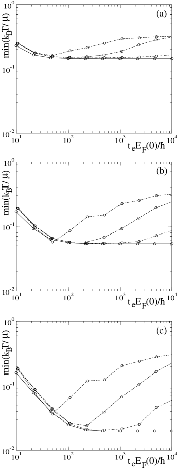
Figure 1: Shown is the minimum value of $k_{\mathrm{B}}T/\mu$ as a function of the time step $t_{e}E_{\mathrm{F}}/\hbar$ for a ⁷Li – ⁶Li mixture and $\hbar\gamma_{\mathrm{coll}}/E_{\mathrm{F}}(0)=\frac{3}{8}\times 10^{-5}$. The ratio $\gamma_{\mathrm{loss}}/\gamma_{\mathrm{coll}}(0)$ is $8/3\times 10^{-2}$, $8/3\times 10^{-3}$, and $8/3\times 10^{-4}$ in panels (a), (b), and (c), respectively. The case of a finite system, Eq. (15), is shown for $10^{2}$ (dashed line), $10^{3}$ (long dashed line), and $10^{4}$ (dot-dashed line) fermions, and the thermodynamic limit, Eq. (23), is shown as a solid line. For the finite system, to the right side of the plot, in the discrete regime, the cooling is blocked; to the left, in the continuous regime, the minimum temperature is dominated by the evaporation rate, according to Eq. (25), and rises as $t_{e}E_{\mathrm{F}}/\hbar$ decreases. The data obtained in the thermodynamic limit are independent of $t_{e}$ except where the evaporation-limited temperature is larger than the loss-limited temperature. Note that the actual data points are represented by open circles fig1note .

Figure 2 shows the effect of $t_{e}$ on the occupation number distribution in energy space. In the continuous regime the distribution clearly depends on energy alone, so that in the thermodynamic limit $N(\mathbf{k})=N(k)$. The distribution is not, however, an equilibrium one, as is more easily observed in the thermodynamic limit (see below). In contrast, in the discrete regime the distribution is fully $\mathbf{k}$-dependent. Careful observation of the figure shows regular holes in the energy spectrum: this is a natural result of the quantization of the box. We note that, in all regimes investigated, the essential feature of a Fermi surface, though distorted, persists.

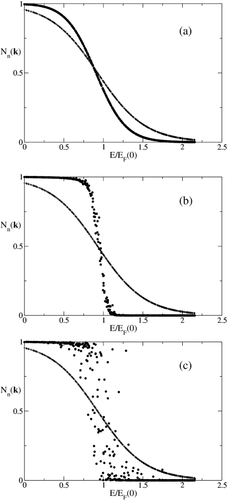
Figure 2: Shown is the mean occupation number for $N_{\mathrm{F}}=1000$ ⁶Li atoms in contact with a ⁷Li reservoir in a finite system. The initial state (plus symbols) is a thermal distribution of $k_{\mathrm{B}}T/\mu=0.324$; $\hbar\gamma_{\mathrm{coll}}/E_{\mathrm{F}}(0)=\frac{3}{8}\times 10^{-5}$. After an evolution time (solid circles) such that $k_{\mathrm{B}}T/\mu$ passes through a minimum according to Eq. (15) with the parameters $\gamma_{\mathrm{loss}}/\gamma_{\mathrm{coll}}(0)=8/3\times 10^{-3}$ and (a) $t_{e}E_{\mathrm{F}}/\hbar=10^{2}$ (continuous regime) (b) $t_{e}E_{\mathrm{F}}/\hbar=10^{3}$, and (c) $t_{e}E_{\mathrm{F}}/\hbar=10^{4}$ (discrete regime), it is clear that in the continuous regime the distribution, though non-thermal, depends only on $|\mathbf{k}|$. In contrast, in the discrete regime the distribution is fully $\mathbf{k}$-dependent.

IV.2 Time Evolution in the Thermodynamic Limit

Figure 3: Time evolution of the number distribution of a Fermi gas sympathetically cooled by a perfect Bose reservoir for two experimentally important cases in the thermodynamic limit: (a) ⁷Li – ⁶Li and (b) ²³Na – ⁶Li. Shown are the initial state of $(k_{\mathrm{B}}T/\mu)(0)=0.7$ (thin line), the state at which the temperature reaches a minimum (thicker line), and a later stage where the gas has heated (thickest line). The hole in the distribution near $k=0$ is particularly evident in panel (b), where the loss processes balance evaporative cooling, as described by Eq. (27). Here $[\gamma_{\mathrm{loss}}/\gamma_{\mathrm{coll}}(0),(k_{\mathrm{B}}T/\mu)_{\mathrm{min}}]=[8.27\times 10^{-3},0.081]$, and $[1.25\times 10^{-2},0.089]$ for panels (a) and (b), respectively, and $\hbar\gamma_{\mathrm{coll}}/E_{\mathrm{F}}(0)=\frac{3}{8}\times 10^{-5}$.

In the thermodynamic limit, as defined explicitly in Sec. IV.1, the sums in Eq. (15) may be approximated using the standard continuum limit

$$\sum_{\mathbf{k}}\rightarrow L^{3}\int\frac{d\mathbf{k}}{(2\pi)^{3}}\,.$$ (21)

As illustrated in Fig. 2, in this limit

$$N(\mathbf{k})=N(k)\,.$$ (22)

The continuum iterative equation for the time evolution may then be written as

$$N_{n+1}(k)=(1-\gamma_{{\rm loss}}\,t_{e})N_{n}(k)+\frac{n_{\mathrm{B}}}{\hbar^{2}}\int_{0}^{+\infty}dk^{\prime}\,k^{\prime 2}$$

$$\times\left\{N_{n}(k)[1-N_{n}(k^{\prime})]\int_{-1}^{+1}du|g(\omega)|^{2}-(k\leftrightarrow k^{\prime})\right\}\,,$$ (23)

where $g(\omega)$ and $\omega$ are defined as in Eqs. (17) and (18) with

$$\mathbf{k}\cdot\mathbf{k}^{\prime}=kk^{\prime}u\,.$$ (24)

Two effects limiting the choice of $t_{e}$ are implicit in Eq. (23). The first, which appears when $t_{e}$ is small, is the width of the interaction function $g(\omega)$: as $k_{\mathrm{B}}T$ approaches the width $4\pi\hbar/t_{e}$ in the course of cooling, the sharp decrease in $N_{n}(k)$ from unity to zero, typical of a Fermi or Fermi-like distribution, is no longer resolved, and the transfer of momentum from fermions to bosons ceases to have any effect on the temperature. This gives an absolute minimum temperature of

$$T_{\mathrm{min}}^{\mathrm{evap}}\sim\frac{\hbar}{t_{e}}\,.$$ (25)

The superscript “evap” refers to the fact that $1/t_{e}$ is the evaporation rate. The second effect, which occurs in the limit of large $t_{e}$, is the validity of perturbation theory, according to Eq. (4). Since this limitation is imposed by our use of perturbation theory it is not fundamental to sympathetic cooling technicalities . Therefore, in practice, within the context of our model, one should choose an evaporation rate such that

$$\frac{T_{\mathrm{F}}}{T}\ll t_{e}E_{\mathrm{F}}/\hbar\ll\frac{T_{\mathrm{F}}}{T}\frac{E_{\mathrm{F}}}{\gamma_{{\rm coll}}\hbar}\,.\,$$ (26)

We have verified that the results are independent of values of $t_{e}$ which satisfy Eq. (26), as illustrated by the plateau in Fig. 1.

It is convenient to begin with $N_{0}(k)$ in the form of a Fermi distribution (though other initial distributions were studied, with the same qualitative results). In the following simulations, $k_{\mathrm{B}}T/\mu=0.7$ was taken as a starting condition. In Fig. 3 is shown the evolution of the occupation number distribution resulting from Eq. (23) with a choice of $t_{e}$ satisfying Eq. (26) and $\gamma_{\mathrm{loss}}/\gamma_{\mathrm{coll}}(0)=8.27\times 10^{-3}$ and $1.25\times 10^{-2}$ for the experimentally relevant cases of ⁶Li–⁷Li and ⁶Li–²³Na, as shown in panels (a) and (b), respectively. Close inspection of the figure shows that the distribution is non-equilibrium: the thermal tail is missing, and, as can be seen by making a fit to a Fermi distribution (not shown), the rise from $N_{n}(k)=0.5$ towards unity with decreasing $k$ is less sharp than that of a Fermi distribution with the same total energy and number of fermions. There is also a hole near $k=0$, which is difficult to see in Fig. 3(a) but appears strongly in Fig. 3(b). One may observe the existence of this latter feature directly from Eq. (23) as follows.

The evolution of $N_{n}(k=0)$ may be approximated by assuming that $N_{n}(k)$ varies slowly near the origin, which allows one to replace $N_{n}(k^{\prime})$ with $N_{n}(0)$ in Eq. (23). The condition that the value of $N_{n}(0)$ increase is then

$$\frac{\gamma_{{\rm loss}}}{\gamma_{{\rm coll}}} \lesssim \frac{4C}{3\pi}[1-N(0)]\left(\frac{\hbar}{\alpha E_{F}t_{e}}\right)^{1/2}(1+\alpha^{2})$$ (27)

$$\times\left[\frac{1}{|1-\alpha|^{3/2}}-\frac{1}{(1+\alpha)^{3/2}}\right]\,,$$

where $\alpha\equiv m_{\mathrm{B}}/m_{\mathrm{F}}$ and $C\equiv 1.860266\ldots$. It is therefore directly apparent that for sufficient loss rates the number distribution has a hole at $k=0$. Moreover, since a factor of $[1-N_{n}(0)]$ enters into the condition, the number distribution never reaches unity at $k=0$ and the distribution is never a Fermi distribution. It was observed numerically that this feature extends up to a finite $k$, the width of which varies dynamically and increases as $m_{\mathrm{B}}/m_{\mathrm{F}}$ takes a value largely different from unity. The deepest point occurs at $k=0$, and the maximum in time of $N_{n}(0)$ is given by replacing the less than or about equal to sign with an equal sign in Eq. (27). The evolution of the hole for a ²³Na–⁶Li mixture is particularly apparent, since $\alpha\simeq 23/6$ is far from unity, which reduces the value of the right hand side of Eq. (27) for a fixed value of $N_{n}(0)$, as illustrated in Fig. 3(b).

The effect of the choice of $\gamma_{\mathrm{loss}}/\gamma_{\mathrm{coll}}$ on the minimal temperature is shown in Fig. 4. The power laws

$$\,\left(\frac{k_{\mathrm{B}}T}{\mu}\right)_{\mathrm{min}}=0.659\left(\frac{\gamma_{\mathrm{loss}}}{\gamma_{\mathrm{coll}}}\right)^{0.436}+5.6\times 10^{-4}$$ (28)

$$\left(\frac{k_{\mathrm{B}}T}{\mu}\right)_{\mathrm{min}}=0.621\left(\frac{\gamma_{\mathrm{loss}}}{\gamma_{\mathrm{coll}}}\right)^{0.445}+7.34\times 10^{-8}$$ (29)

for ⁷Na–⁶Li and ²³Na–⁶Li, respectively, were found over the range $8/3\times 10^{-5}\leq\gamma_{\mathrm{loss}}/\gamma_{\mathrm{coll}}\leq 8/3\times 10^{-2}$. Note that the constant offsets in the above are negligible over the fit domain. Although the distributions shown in Fig. 3 are not Fermi distributions, the step-like feature makes a temperature and chemical potential, as defined by the total number of particles and the total energy, a meaningful measure of the shape of $N_{n}(k)$. Moreover, as $N_{\mathrm{F}}^{\mathrm{tot}}$ and $E_{\mathrm{F}}^{\mathrm{tot}}$ are weighted by $k^{2}$ and $k^{4}$ respectively, the hole near $k=0$ has little effect on them.

Figure 4: The numerically determined maximum Fermi degeneracy as a function of loss rate for ⁷Li – ⁶Li (open circles) and ²³Na – ⁶Li (black diamonds) mixtures in the thermodynamic limit, according to the quantum Boltzmann equation. One finds $(k_{\mathrm{B}}T/\mu)_{\mathrm{min}}\propto(\gamma_{\mathrm{loss}}/\gamma_{\mathrm{coll}}(0))^{0.44}$. The dashed line shows the analytic prediction of $(k_{\mathrm{B}}T/\mu)_{\mathrm{min}}\propto(\gamma_{\mathrm{loss}}/\gamma_{\mathrm{coll}}(0))^{1/3}$ based on the assumption of a Fermi distribution. The difference is due to the non-thermal nature of the quasi-static mean occupation number distribution, an example of which is illustrated in Fig. 3. Here $\hbar\gamma_{\mathrm{coll}}/E_{\mathrm{F}}(0)=\frac{3}{8}\times 10^{-5}.$

Figure 5: Time evolution of the degeneracy in the thermodynamic limit as determined by numerical evolution of Eq. (23) (solid line), and the analytical prediction of Eq. (37) (dashed line) based on a Fermi ansatz. The parameters are $\gamma_{\mathrm{loss}}/\gamma_{\mathrm{coll}}(0)=8.27\times 10^{-3}$, $(k_{\mathrm{B}}T/\mu)(0)=0.7$, $t_{e}E_{\mathrm{F}}(0)\hbar=10^{3}$, and $\hbar\gamma_{\mathrm{coll}}/E_{\mathrm{F}}(0)=\frac{3}{8}\times 10^{-5}$.

Finally, Fig. 5 illustrates the time evolution of $k_{\mathrm{B}}T/\mu$ for the parameters $\gamma_{\mathrm{loss}}/\gamma_{\mathrm{coll}}(0)=8.27\times 10^{-3}$ and $t_{e}E_{\mathrm{F}}(0)\hbar=10^{3}$. The figure is divided into three time regions which show three phases of the evolution: cooling, the achievment of a minimal $k_{\mathrm{B}}T/\mu$, and heating. These three regions were observed in all simulations for which $\gamma_{\mathrm{loss}}/\gamma_{\mathrm{coll}}\ll 1$, and were independent of $t_{e}E_{F}/\hbar$ within the constraints of Eq. (26).

IV.3 Analytical Prediction of the Degeneracy for a Fermi Distribution Ansatz

The following concerns the thermodynamic limit alone. In the limit in which

$$\hbar/t_{e}\ll k_{\mathrm{B}}T\,,\,$$ (30)

one may use the approximation

$$|g(\omega)|^{2}\sim\frac{3\pi}{4}g_{0}^{2}t_{e}\delta(\omega)\,,$$ (31)

where $\delta(\omega)$ is a Dirac delta distribution. Substituting Eq. (31) into Eq. (23), and defining time continuously according to

$$\dot{N}(k,t)\equiv\frac{N_{n+1}-N_{n}}{t_{e}}\,,\,$$ (32)

the iterative rate equation reduces to a first order partial integro-differential equation with an integration over $k^{\prime}$ alone:

$$\dot{N}(k,t)=-\gamma_{{\rm loss}}N(k,t)+\frac{3}{8}\,\frac{n_{\mathrm{B}}g_{0}^{2}m_{\mathrm{B}}}{2\pi\hbar^{3}}$$

$$\times\left\{\int_{k}^{\left|\frac{1+\alpha}{1-\alpha}\right|k}dk^{\prime}\,\frac{k^{\prime}}{k}N(k^{\prime},t)[1-N(k,t)]\right.$$

$$-\left.\int_{\left|\frac{1-\alpha}{1+\alpha}\right|k}^{k}dk^{\prime}\,\frac{k^{\prime}}{k}[1-N(k^{\prime},t)]N(k,t)\right\}\,,$$ (33)

where $\alpha\equiv m_{\mathrm{B}}/m_{\mathrm{F}}$. Here the functional form of the limits of integration was determined by integration of the delta distribution over the solid angle. Note that in the limit in which $k\rightarrow 0$, $\dot{N}(k)=-\gamma_{{\rm loss}}N_{n}(k)$, provided that $m_{\mathrm{F}}\neq m_{\mathrm{B}}$. In the limit as $m_{\mathrm{B}}\rightarrow m_{\mathrm{F}}\equiv m$, the limits of integration of Eq. (33) simplify to $[k,\infty]$ and $[0,k]$, respectively. In this case the $1/k$ in the integrand is not regulated and the expression diverges as $k\rightarrow 0$, save in the case where $[1-N(k)]\rightarrow 0$.

An analytical model of the time evolution of the temperature can be developed based on a Fermi distribution ansatz, namely,

$$N_{a}(k,t)\equiv\frac{1}{\exp\left\{\left[\frac{\hbar^{2}k^{2}}{2m}-\mu(t)\right]/k_{\mathrm{B}}T(t)\right\}+1}\,.\,$$ (34)

For simplicity, the case $m\equiv m_{\mathrm{F}}=m_{\mathrm{B}}$ is considered. Two equations for the unknowns $T(t)$ and $\mu(t)$ are obtained by multiplying Eq. (33) by $k^{0}$ and $k^{2}$ and integrating over $\mathbf{k}$:

$$\frac{d}{dt}N_{\mathrm{F}}^{\mathrm{tot}}(t) = -\gamma_{\mathrm{loss}}N_{\mathrm{F}}^{\mathrm{tot}}\,,\,$$ (35)

$$\frac{d}{dt}E_{\mathrm{F}}^{\mathrm{tot}}(t) = \frac{L^{3}}{(2\pi)^{3}}\int d^{3}k\frac{\hbar^{2}k^{2}}{2m}\dot{N}(k,t)\,,\,$$ (36)

where $N_{\mathrm{F}}^{\mathrm{tot}}$ and $E_{\mathrm{F}}^{\mathrm{tot}}$ are the total number of fermions and total energy of the fermions, respectively. In the degenerate regime where $k_{\mathrm{B}}T/\mu\ll 1$, one may obtain an approximate evolution of $k_{\mathrm{B}}T/\mu$ from Eqs. (35) and (36). One neglects terms of order $\exp(-\mu/k_{\mathrm{B}}T)$ in the right hand side of Eq. (36) and uses the low temperature expansions of $N_{\mathrm{F}}^{\mathrm{tot}}$ and $E_{\mathrm{F}}^{\mathrm{tot}}$ landau3 . Details are given in App. C. One finds

$$\frac{d}{dt}\left(\frac{k_{\mathrm{B}}T}{\mu}\right)^{2}=\frac{8}{5\pi^{2}}\gamma_{\mathrm{loss}}-\frac{12\zeta(3)}{\pi^{2}}\gamma_{\mathrm{coll}}(t)\,\left(\frac{k_{\mathrm{B}}T}{\mu}\right)^{3}\,,\,$$ (37)

which clearly shows the separate contributions of heating due to losses and cooling due to elastic collisions. The fact that the cooling term is proportional to $T^{3}$ has a simple physical interpretation. Each collisional process occurs at a rate $\gamma_{\mathrm{coll}}k_{\mathrm{B}}T/\mu$ due to Pauli blocking. It involves a fraction $k_{\mathrm{B}}T/\mu$ of the total number of fermions. The energy transferred to a boson per collisional event is of order $k_{\mathrm{B}}T$. Therefore the collisional term in $dE/dt$ is proportional to $T^{3}$, from which follows Eq. (37).

In the limit $\gamma_{\mathrm{loss}}/\gamma_{\mathrm{coll}}\ll 1$, which is in fact the experimental case, one may distinguish three different stages in the evolution of $k_{\mathrm{B}}T/\mu$. In the first stage, cooling dominates and it decreases according to the power law

$$\left(\frac{k_{\mathrm{B}}T}{\mu}\right)(t)\sim\frac{1}{6\zeta(3)\pi^{-2}\gamma_{\mathrm{coll}}(0)\,t+(\mu/k_{\mathrm{B}}T)(0)}\,.\,$$ (38)

Note that, in the case where $\gamma_{\mathrm{loss}}=0$, Eq. (38) holds indefinitely. In the second stage, after a time $t_{\mathrm{min}}$, $k_{\mathrm{B}}T/\mu$ arrives at a minima, given by

$$\left(\frac{k_{\mathrm{B}}T}{\mu}\right)_{\mathrm{min}}=\left[\frac{2}{15\zeta(3)}\frac{\gamma_{\mathrm{loss}}}{\gamma_{\mathrm{coll}}(0)}\right]^{1/3}\,,\,$$ (39)

$$t_{\mathrm{min}}\simeq[\gamma_{\mathrm{coll}}(0)]^{-2/3}\gamma_{\mathrm{loss}}^{-1/3}\,.\,$$ (40)

Note that $\gamma_{\mathrm{loss}}t_{\mathrm{min}}\ll 1$, so that a very small fraction of the atoms have been lost when $k_{\mathrm{B}}T/\mu$ achieves its minimum. In the third stage, heating manifests as an adiabatic increase in $k_{\mathrm{B}}T/\mu$, obtained by neglecting $d(k_{\mathrm{B}}T/\mu)^{2}/dt$ in Eq. (33) and thereby replacing $\gamma_{\mathrm{coll}}(0)$ by $\gamma_{\mathrm{coll}}(t)=\gamma_{\mathrm{coll}}(0)\exp(-\gamma_{\mathrm{loss}}t/3)$ in Eq. (39). The evolution of $k_{\mathrm{B}}T/\mu$ continues to increase adiabatically up till a characteristic time given by

$$t_{\mathrm{nonadiabatic}}\sim\frac{3}{\gamma_{\mathrm{loss}}}\ln\left(\frac{\gamma_{\mathrm{coll}}}{\gamma_{\mathrm{loss}}}\right)\,.$$ (41)

Note that, at this evolution time, $k_{\mathrm{B}}T/\mu$ is on the order of unity, and the above analytical treatment ceases to be applicable.

The number $\Delta N_{\mathrm{B}}$ of bosons lost from the reservoir during the first and second stages of cooling, i.e., up till the time at which the minimum $k_{\mathrm{B}}T/\mu$ is achieved, may be estimated simply from Eq. (38). One integrates the rate of production of excited bosons $\propto N_{\mathrm{F}}(0)(k_{\mathrm{B}}T/\mu)^{2}\gamma_{\mathrm{coll}}(0)$ over time, and finds the approximate relation

$$\Delta N_{\mathrm{B}}\propto N_{\mathrm{F}}(0)\left(\frac{k_{\mathrm{B}}T}{\mu}\right)(0).$$ (42)

This corresponds to the initial number of fermions active in the cooling process.

In Fig. 4 is shown the minimum temperature as a function of loss rate. The difference between the analytical prediction of Eq. (39) (dashed line) and the numerical results of Eq. (23) (solid line) highlight the non-equilibrium nature of the actual mean occupation number distribution. However, the qualitative features are the same for both the analytical model and the numerical simulation. Figure 5 shows the evolution for the parameters $\gamma_{\mathrm{loss}}/\gamma_{\mathrm{coll}}(0)=8.27\times 10^{-3}$ and $(k_{\mathrm{B}}T/\mu)(0)=0.7$. The three stages of cooling, achievement of a minimum temperature, and heating, are clearly observable. As $\gamma_{\mathrm{loss}}/\gamma_{\mathrm{coll}}(0)\ll 1$, the time scale of the first stage is small compared to the third stage.

V Beyond the Boltzmann approximation: the Master Equation

The quantum Boltzmann equation is a closed equation obtained after use of Wick’s theorem to replace the mean value of occupation numbers with the product of their mean values. Such an approximation applies when the probability distribution of the density operator is nearly Gaussian gardiner1997 ; jaksch1997 , and neglects correlations between modes. In the following, the exact probability distribution of the occupation number shall be treated by deriving a master equation for the fermion density operator in the limit of weak coupling. Specifically, $g_{0}$ must be small enough so that the probability to have more than one boson excited out of the condensate during $t_{e}$ is negligible. In the Fock basis, the density operator is characterized both by ‘populations’ and ‘coherences’, that is, by the diagonal and off-diagonal matrix elements, respectively. Subsequently, the secular approximation will be used to derive an equation for the evolution of the distribution probability of the occupation numbers. This approximation applies in the regime in which the evolution rate of the populations is much smaller than the Bohr frequency of the coherences cohentannoudji1 , which allows one to derive closed equations for the populations.

V.1 Derivation of the Quantum Boltzmann Master Equation

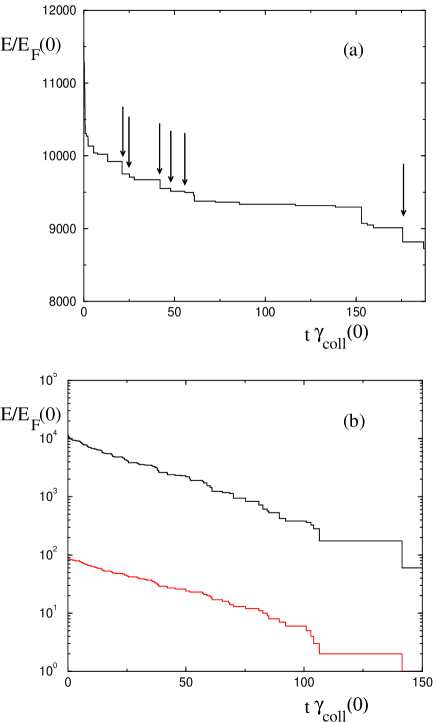
Figure 6: Evolution of the total energy of the fermions for a finite system for one Monte-Carlo realization of the exact occupation number distribution under the secular approximation (see text) according to Eq. (57). (a) $\gamma_{\mathrm{loss}}/\gamma_{\mathrm{coll}}(0)=8/3\times 10^{-4}$: the loss events (in this case 6) are marked by arrows. Clearly cooling dominates the decrease in the energy at early times while loss plays a stronger role at later times. (b) $\gamma_{\mathrm{loss}}/\gamma_{\mathrm{coll}}(0)=8/3\times 10^{-2}$: The upper curve shows the evolution of the energy, and the lower curve shows the evolution of the number of atoms. At early times, the slope of the energy is compounded of the effect of cooling and a trivial decrease of the Fermi energy $\propto\exp(-2\gamma_{\mathrm{loss}}t/3)$ due to atom loss. In both (a) and (b), $(k_{\mathrm{B}}T/\mu)(0)=0.324$, $N_{\mathrm{F}}(0)=100$, $t_{e}E_{\mathrm{F}}/\hbar=10^{3}$.

Figure 7: The numerically determined maximum Fermi degeneracy as a function of loss rate for $N=100$ (dashed line) and $N=1000$ (solid line) ⁶Li fermions in contact with ⁷Li (open circles) or ²³Na (black diamonds), according to the quantum master Boltzmann equation. The value of $t_{e}E_{\mathrm{F}}/\hbar$ which gives the minimal temperature has been chosen. Arrows indicate the long term cooling limits for $\gamma_{\mathrm{loss}}=0$ for ⁷Li–⁶Li and ²³Na–⁶Li mixes, respectively. The minimal temperature is much higher in comparison to that predicted by the quantum Boltzmann equation in the thermodynamic limit, as was shown in Fig. 4 (note scale change).

Just after a measurement of state of the bosons, but before excited bosons have been removed from the system via evaporation, the fermion density operator may be written

$$\tilde{\rho}_{\mathrm{F}}[(n+1)t_{e}]=\langle N_{\mathrm{B}}:\mathbf{0}|\tilde{\rho}[(n+1)t_{e}]|N_{\mathrm{B}}:\mathbf{0}\rangle$$

$$+\sum_{\mathbf{q}\neq\mathbf{0}}\langle N_{\mathrm{B}}-1:\mathbf{0};1:\mathbf{q}|\tilde{\rho}[(n+1)t_{e}]|N_{\mathrm{B}}-1:\mathbf{0};1:\mathbf{q}\rangle\,,$$ (43)

where a sum over bosonic Fock states has been taken. By choosing $g_{0}$ sufficiently small one may indeed neglect the possibility of exciting more than one boson out of the condensate. The first term in Eq. (43) represents zero excited bosons, and the second term a single excited boson of momentum $\hbar\mathbf{q}$. The combined bosonic and fermionic density operator $\tilde{\rho}[(n+1)t_{e}]$ is given by the action on Eq. (12) of the evolution operator $\tilde{U}(nt_{e})$ from time $nt_{e}$ to time $(n+1)t_{e}$:

$$\tilde{\rho}[(n+1)t_{e}]=$$ (44)

$$\tilde{U}(nt_{e})\left[\tilde{\rho}_{\mathrm{F}}(nt_{e}^{-})\otimes|N_{\mathrm{B}}:\mathbf{q}=\mathbf{0}\rangle\langle N_{\mathrm{B}}:\mathbf{q}=\mathbf{0}|\right]\tilde{U}^{\dagger}(nt_{e})\,.$$

One then expands the evolution operator $\tilde{U}(nt_{e})$ to second order in the interaction potential $V$ using standard time-dependent perturbation theory, which results in the second order expansion of Eq. (44), and thus Eq. (43).

One obtains the following operators which act on the fermions alone:

$$C_{\mathbf{q}}(nt_{e}) \equiv \int_{nt_{e}}^{(n+1)t_{e}}\frac{dt^{\prime}}{i\hbar}$$ (45)

$$\langle N_{\mathrm{B}}-1:\mathbf{0},1:\mathbf{q}|\tilde{V}(t^{\prime})|N_{\mathrm{B}}:\mathbf{0}\rangle\,,$$

$$A(nt_{e}) \equiv \int_{nt_{e}}^{(n+1)t_{e}}\frac{dt^{\prime}}{i\hbar}\int_{nt_{e}}^{t^{\prime}}\frac{dt^{\prime\prime}}{i\hbar}$$ (46)

$$\langle N_{\mathrm{B}}:\mathbf{0}|\tilde{V}(t^{\prime})\tilde{V}(t^{\prime\prime})|N_{\mathrm{B}}:\mathbf{0}\rangle\,.$$

$C_{\mathbf{q}}$ may be written explicitly as

$$C_{\mathbf{q}}(nt_{e})=\frac{\sqrt{N_{\mathrm{B}}}}{i\hbar}\sum_{\mathbf{k}}g(\omega)e^{i\omega nt_{e}}c^{\dagger}_{\mathbf{k}-\mathbf{q}}c_{\mathbf{k}}\,,$$ (47)

$$\omega\equiv\frac{\hbar(\mathbf{k}-\mathbf{q})^{2}}{2m_{\mathrm{F}}}+\frac{\hbar q^{2}}{2m_{\mathrm{B}}}-\frac{\hbar k^{2}}{2m_{\mathrm{F}}}\,.$$ (48)

The explicit form of $A$ is more complicated, but may be derived by substituting Eq. (2) into Eq. (46). $C_{\mathbf{q}}$ originates from the second term of Eq. (43) in which one boson is excited. It originates from a first order perturbative expansion of $\tilde{U}$, but appears in two factors of Eq. (44) and therefore gives a contribution of order $g_{0}^{2}$ in the evolution of the density operator. $A$ originates from the first term in Eq. (43) with the evolution operator expanded to second order in $g_{0}$. It contains, in particular, an effective interaction between fermions mediated by the bosons. This results in the master equation for the fermionic density operator

$$\tilde{\rho}_{\mathrm{F}}[(n+1)t_{e}]=\tilde{\rho}_{\mathrm{F}}(nt_{e})+A(nt_{e})\tilde{\rho}_{\mathrm{F}}(nt_{e})$$

$$+\tilde{\rho}_{\mathrm{F}}(nt_{e})A^{\dagger}(nt_{e})+\sum_{\mathbf{q}\neq\mathbf{0}}C_{\mathbf{q}}(nt_{e})\tilde{\rho}_{\mathrm{F}}(nt_{e})C^{\dagger}_{\mathbf{q}}(nt_{e})\,.$$ (49)

We now proceed to apply the secular approximation cohentannoudji1 . To illustrate the details, the contribution of $C_{\mathbf{q}}$ is described explicitly. Evaluating the last term in Eq. (49),

$$[C_{\mathbf{q}}\tilde{\rho}_{\mathrm{F}}C^{\dagger}_{\mathbf{q}}](nt_{e})=\frac{N_{\mathrm{B}}}{\hbar^{2}}\sum_{\mathbf{k}_{1},\mathbf{k}_{2}}e^{i(\omega_{1}-\omega_{2})nt_{e}}$$

$$g(\omega_{1})g^{*}(\omega_{2})c^{\dagger}_{\mathbf{k}_{1}-\mathbf{q}}c_{\mathbf{k}_{1}}\tilde{\rho}_{\mathrm{F}}(nt_{e})c^{\dagger}_{\mathbf{k}_{2}}c_{\mathbf{k}_{2}-\mathbf{q}}\,,$$ (50)

where $\omega_{1,2}$ is defined as in Eq. (48), with $\mathbf{k}$ replaced by $\mathbf{k}_{1,2}$. The typical evolution rate $\gamma_{\mathrm{evolve}}$ of the fermionic density operator is proportional to $g_{0}^{2}$. In contrast, the Bohr frequencies $\omega_{1}-\omega_{2}$ do not depend on $g_{0}$. Therefore the oscillating exponential in Eq. (50) may be neglected for sufficiently small $g_{0}$, as its effects averages to zero when averaged during $1/\gamma_{\mathrm{evolve}}$. An estimate for $\gamma_{\mathrm{evolve}}$ may be made based on the assumption of a thermal distribution in the thermodynamic limit, as defined by Eq. (20):

$$\gamma_{\mathrm{evolve}}=\frac{\delta N_{\mathrm{B}}}{t_{e}}\simeq\gamma_{\mathrm{coll}}N_{\mathrm{F}}\left(\frac{T}{T_{\mathrm{F}}}\right)^{2}\,,$$ (51)

where $\delta N_{\mathrm{B}}\ll 1$ is the mean number of excited bosons during one cycle of duration $t_{e}$. The minimal Bohr frequencies are given by

$$\mathrm{min}(|\omega_{1}-\omega_{2}|)\simeq\frac{1}{\hbar\rho(E_{\mathrm{F}})}=\left(\frac{2\pi}{L}\right)^{3}\frac{\hbar}{4\pi mk_{\mathrm{F}}}\,,$$ (52)

where $\rho(E_{\mathrm{F}})$ is the density of states at the Fermi surface. Therefore the condition for validity of the secular approximation is

$$\frac{\hbar\gamma_{\mathrm{coll}}}{E_{\mathrm{F}}}N_{\mathrm{F}}^{2}\left(\frac{T}{T_{\mathrm{F}}}\right)^{2}\ll 1\,,$$ (53)

for which, in Eq. (50), one keeps only the terms with $\omega_{1}=\omega_{2}$. Assuming the box lengths squared to be incommensurable, one finds

$$q_{\alpha}=0\>\>\>\mathrm{or}\>\>\>k_{1\alpha}=k_{2\alpha}\,,$$ (54)

for each $\alpha\in\{x,y,z\}$. The former case, which corresponds to the excitation of a boson in the plane orthogonal to $\alpha$, we neglect. The existence of this solution is a consequence of the separability of the degrees of motion along $x,y,z$ in the box. One could consider an alternate model for the box in which this separability is lifted to justify its being neglected santos1999b . There therefore remains the sole condition $\mathbf{k}_{1}=\mathbf{k}_{2}$.

Having applied the secular approximation, if $\tilde{\rho}_{\mathrm{F}}$ is initially a statistical mixture of Fock states, then it remains one for all times. Defining the occupation number probability distribution $Q_{n}(\{n_{\mathbf{k}}\})$ by

$$\tilde{\rho}_{\mathrm{F}}(nt_{e})=\sum_{\{n_{\mathbf{k}}\}}Q_{n}(\{n_{\mathbf{k}}\})|\{n_{\mathbf{k}}\}\rangle\langle\{n_{\mathbf{k}}\}|\,,\,$$ (55)

where

$$|\{n_{\mathbf{k}}\}\rangle\equiv\prod_{\mathbf{k}}\left(\hat{c}_{\mathbf{k}}^{\dagger}\right)^{n_{\mathbf{k}}}|\mathrm{vac}\rangle\,,\,$$ (56)

and each $n_{\mathbf{k}}\in\{0,1\}$, one obtains the equation of motion for $Q$:

$$Q_{n+1}(\{n_{\mathbf{k}}\})-Q_{n}(\{n_{\mathbf{k}}\})=\sum_{\mathbf{k_{1}}\neq\mathbf{k_{2}}}\frac{N_{\mathrm{B}}|g(\omega)|^{2}}{\hbar^{2}L^{6}}\left\{-n_{\mathbf{k_{1}}}(1-n_{\mathbf{k_{2}}})Q_{n}(\{n_{\mathbf{k}}\})+n_{\mathbf{k_{2}}}(1-n_{\mathbf{k_{1}}})Q_{n}(\{n_{\mathbf{k}}+\delta_{\mathbf{k},\mathbf{k_{1}}}-\delta_{\mathbf{k},\mathbf{k_{2}}}\})\right\}$$

$$-\left(\sum_{\mathbf{k_{0}}}\gamma_{\mathrm{loss}}t_{e}n_{\mathbf{k_{0}}}\right)Q(\{n_{\mathbf{k}}\})+\left[\sum_{\mathbf{k_{0}}}\gamma_{\mathrm{loss}}t_{e}(1-n_{\mathbf{k_{0}}})\right]Q(\{n_{\mathbf{k}}+\delta_{\mathbf{k},\mathbf{k_{0}}}\})\,,\,$$ (57)

with

$$\hbar\omega\equiv\frac{\hbar^{2}k_{2}^{2}}{2m_{\mathrm{F}}}+\frac{\hbar^{2}(\mathbf{k_{1}}-\mathbf{k_{2}})^{2}}{2m_{\mathrm{B}}}-\frac{\hbar^{2}k_{1}^{2}}{2m_{\mathrm{F}}}\,.\,$$ (58)

Here the loss term has been added in by hand under the assumption that $\gamma_{\mathrm{loss}}t_{e}N_{\mathrm{F}}\ll 1$. The condition that the number of bosons excited during $t_{e}$ be much smaller than unity may be written

$$\sum_{\mathbf{k_{1}},\mathbf{k_{2}}}\mathcal{P}(\mathbf{k_{1}}\rightarrow\mathbf{k_{2}})n_{\mathbf{k_{1}}}(1-n_{\mathbf{k_{2}}})\ll 1\,,$$ (59)

for typical configurations $\{n_{\mathbf{k}}\}$, where $\mathcal{P}$ is defined as in Eq. (16). This is to be contrasted with the much weaker condition of Eq. (19) obtained in the Quantum Boltzmann equation, where the sum is over only one momentum.

V.2 Monte Carlo Numerical Study

The continuous time version of Eq. (57), where $Q_{n+1}-Q_{n}\equiv t_{e}\dot{Q}$, was studied numerically via Monte Carlo simulation. All data for $N_{\mathrm{F}}(0)=10^{2}$ and $N_{\mathrm{F}}(0)=10^{3}$ in Fig. 1 was re-evaluated, with a mean over 100 realizations of $Q$ made for each data point. The qualitative features of the evolution of the mean number distribution were found to remain the same: its non-equilibrium nature, as illustrated for the finite system in Fig. 2 and for the thermodynamic limit in Fig. 3; and the three evolution stages of rapid cooling, achievement of a minimum, and slow heating with a quasi-static distribution, as illustrated for the thermodynamic limit in Fig. 5. Two examples of a single Monte-Carlo realization are illustrated in Fig. 6. The minimum temperature for these simulations is achieved at $\gamma_{\mathrm{coll}}(0)\,t\sim 20$. Before this time the evolution of the energy is dominated by cooling, rather than losses: in Fig. 6(a) this is directly apparent, as the loss of individual fermions is marked by arrows; in Fig. 6(b), where the loss rate was higher, the slope is seen to be different from that which results from the mere evolution of the total number of fermions, the latter of which is determined according to $\langle N_{\mathrm{F}}^{\mathrm{tot}}\rangle=N_{\mathrm{F}}^{\mathrm{tot}}(0)\exp(-\gamma_{\mathrm{loss}}t)$. After this time loss dominates, as is apparent in both panels: the greater part of the changes in the energy occur at the same time as loss of a fermion.

However, quantitatively the agreement between the results of the quantum Boltzmann equation and the quantum Boltzmann master equation depends both on the number of atoms and on the evaporation rate. For 100 atoms, the minimum temperature predicted by the master equation, as shown in Fig. 7, is as much as 50% higher as for the same parameters as in Fig. 1. This deviation is strongest for small loss rates, where the cooling efficiency is limited by the blocking mechanism due to the discrete nature of the spectrum, as discussed in Sec. IV.1. For 1000 atoms, the agreement is very good for the loss rates of Figs. 1(a) and 1(b) while for Fig. 1(c) there is a 15% increase in the temperature. The power laws

$$\,\left(\frac{k_{\mathrm{B}}T}{\mu}\right)_{\mathrm{min}}=0.861\left(\frac{\gamma_{\mathrm{loss}}}{\gamma_{\mathrm{coll}}}\right)^{0.503}+1.44\times 10^{-2}$$ (60)

$$\left(\frac{k_{\mathrm{B}}T}{\mu}\right)_{\mathrm{min}}=0.855\left(\frac{\gamma_{\mathrm{loss}}}{\gamma_{\mathrm{coll}}}\right)^{0.518}+0.993\times 10^{-2}$$ (61)

for ⁷Li–⁶Li and ²³Na–⁶Li, respectively, were found over the full range of data shown in Fig. 7 for $N=1000$. Comparing to Eqs. (29) and (29), which were obtained in the thermodynamic limit with the quantum Boltzmann equation, one observes that the exponents of the power law are similar, whereas the constant offset is substantially different. Recalling that the data of Fig. 7 resulted from an optimization over $t_{e}$, this suggests that even in the absence of loss there is an absolute minimal temperature of $k_{\mathrm{B}}T/\mu\sim 10^{-2}$. This was validated for 1000 atoms by Monte Carlo simulations with a zero loss rate, as indicated by arrows drawn along the left hand $y$-axis of the figure: for ⁷Li–⁶Li, $\mathrm{min}(k_{\mathrm{B}}T/\mu)=1.34\times 10^{-2}$; for ²³Na–⁶Li, $\mathrm{min}(k_{\mathrm{B}}T/\mu)=0.98\times 10^{-2}$.

Therefore, by taking the actual probability distribution for the occupation numbers into account, i.e., by not assuming near-thermal equilibrium according to Wick’s theorem, it is found that the minimum temperature increases when loss does not dominate the cooling. This again highlights the non-thermal nature of this system. In contrast, when $N_{\mathrm{F}}$ is large and the loss rate is in the experimental range of $10^{-2}\gamma_{\mathrm{coll}}$ to $10^{-3}\gamma_{\mathrm{coll}}$, the secular approximation shows that Wick’s theorem is a valid assumption and one may simply use the quantum Boltzmann equation.

VI Conclusion

We have investigated the effect of heating caused by loss of atoms on the minimum temperature that may be achieved in a sympathetically cooled Fermi gas. The model of sympathetic cooling that we have used is cyclical and consists of a sequence of time intervals during which fermions are coupled to a zero-temperature ideal Bose gas via binary atomic interactions. At the end of each time interval the excited bosons are removed from the system by evaporation. The length of the time interval is short enough that the bosons do not come into thermal equilibrium with the fermions; this is in contrast to present experiments in which the bosons and fermions are always in equilibrium with one another. The cooling is balanced by a constant loss rate of fermions, which, for example, can be caused by collisions with background gas in the experimental apparatus, and can lead to heating, as shown in Ref. timmermans2 . The combination of cooling and heating are modeled at several levels of theoretical approximation.

First, a quantum Boltzmann equation describing the evolution of the mean occupation number distribution was developed under the assumption that the fermion density operator is nearly Gaussian, i.e., that Wick’s theorem may be applied. The overall minimum temperature, which was found to be best obtained in the thermodynamic limit, was observed to follow the power law $(k_{\mathrm{B}}T/\mu)_{\mathrm{min}}\sim 0.65(\gamma_{\mathrm{loss}}/\gamma_{\mathrm{coll}})^{0.44}$, so that $(k_{\mathrm{B}}T/\mu)_{\mathrm{min}}\lesssim 0.03$ for $\gamma_{\mathrm{loss}}/\gamma_{\mathrm{coll}}\leq 10^{-3}$, where $\mu\sim k_{\mathrm{B}}T_{\mathrm{F}}$ is the chemical potential of the fermions, $\gamma_{\mathrm{coll}}$ is the bare fermion–boson collision rate not including the reduction due to Fermi statistics, and $\gamma_{\mathrm{loss}}$ is the constant fermion loss rate. This value of $\gamma_{\mathrm{loss}}/\gamma_{\mathrm{coll}}$ is easily achievable in present experiments, in particular by using a Feshbach resonance Inguscio . The number distribution was observed to have a distorted Fermi surface and a hole near $\mathbf{k}=0$.

A second theoretical perspective was developed based on the secular approximation to a master equation, without the use of Wick’s theorem. Monte Carlo simulations of the resulting quantum Boltzmann master equation showed that in the limit of experimentally reasonable values of $\gamma_{\mathrm{loss}}/\gamma_{\mathrm{coll}}$ and the number of fermions $N_{\mathrm{F}}$, the first theoretical approach is indeed valid. However, for values of $\gamma_{\mathrm{loss}}/\gamma_{\mathrm{coll}}$ tending towards zero, the master equation shows a substantially higher temperature. In the most extreme case studied of 100 atoms and $\gamma_{\mathrm{loss}}/\gamma_{\mathrm{coll}}=3\times 10^{-4}$, this increase is 50%.

A possible extension to this work is to add a harmonic trap and/or to include interactions between bosons. The assumption of a perfect Bose reservoir is reasonable when the speed of sound is much smaller than the Fermi velocity timmermans1998 , as is the case for weakly interacting condensates. Although a harmonic trap may change the predicted minimal temperature, the qualitative results of this study are expected to be correct even for a non-uniform system such as is found in present experiments on Fermi–Bose mixtures.

Acknowledgments: We would like to thank Jean Dalibard for proposing this project, Christophe Salomon for useful discussions, and Murray Holland for a very useful remark. This work was supported by NSF grant no. MPS-DRF 0104447. Laboratoire Kastler Brossel is a research unit of l’École normale supérieure and of l’Université Pierre et Marie Curie, associated with CNRS. We acknowledge financial support from Région Ile de France.

Appendix A Evolution of the occupation numbers

In the following, we will calculate an approximation to the variation of the expectation value of the number operator

$$\zeta_{0}=\hat{c}^{\dagger}_{\mathbf{k_{0}}}\hat{c}_{\mathbf{k_{0}}}$$ (62)

from time $nt_{e}$ to time $(n+1)t_{e}$, that is, during the time interval of duration $t_{e}$ between two successive measurements of the state of the bosons.

One begins with the approximate evolution of the number operator obtained using second order perturbation theory for $\Lambda$, Eq. (11). One takes the expectation of Eq. (11) with respect to the density operator Eq. (12). All the bosons at time $nt_{e}$ are in the state with zero momentum. In order to take the expectation value first with respect to the bosons, it is convenient to rewrite the interaction potential $V$ as

$$\tilde{V}(t)=\sum_{\mathbf{q}\neq\mathbf{q}^{\prime}}W_{\mathbf{q}\mathbf{q}^{\prime}}(t)\hat{b}_{\mathbf{q}^{\prime}}^{\dagger}\hat{b}_{\mathbf{q}}$$ (63)

where the $W$’s are purely fermionic operators:

$$W_{\mathbf{q}^{\prime}\mathbf{q}}(t)=\frac{g_{0}(t)}{L^{3}}\sum_{\mathbf{k}\neq\mathbf{k}^{\prime}}e^{i\Omega_{\mathbf{k}^{\prime}\mathbf{q}^{\prime},\mathbf{k}\mathbf{q}}t}\hat{c}^{\dagger}_{\mathbf{k}^{\prime}}\hat{c}_{\mathbf{k}}\delta_{\mathbf{k}+\mathbf{q},\mathbf{k}^{\prime}+\mathbf{q}^{\prime}}\,,$$ (64)

with

$$\Omega_{\mathbf{k}^{\prime}\mathbf{q}^{\prime},\mathbf{k}\mathbf{q}}\equiv\frac{\hbar k^{{}^{\prime}2}}{2m_{\mathrm{F}}}+\frac{\hbar q^{{}^{\prime}2}}{2m_{\mathrm{B}}}-\frac{\hbar k^{2}}{2m_{\mathrm{F}}}-\frac{\hbar q^{2}}{2m_{\mathrm{B}}}.$$ (65)

Expanding the commutators in (12) and using the fact that $\tilde{V}$ does not contain terms with $\mathbf{q}=\mathbf{q}^{\prime}$, one obtains the following matrix elements and their expressions:

$$\langle N_{\mathrm{B}}:\mathbf{0}|\tilde{V}(t)|N_{\mathrm{B}}:\mathbf{0}\rangle=0$$ (66)

$$\langle N_{\mathrm{B}}:\mathbf{0}|\tilde{V}(t)\ldots\tilde{V}(t^{\prime})|N_{\mathrm{B}}:\mathbf{0}\rangle$$

$$=N_{\mathrm{B}}\sum_{\mathbf{q}^{\prime}\neq\mathbf{0}}W_{\mathbf{0},\mathbf{q}^{\prime}}(t)\ldots W_{\mathbf{q}^{\prime},\mathbf{0}}(t^{\prime})$$ (67)

where $(\ldots)$ may contain an operator acting on the fermions alone. These results may be interpreted physically as follows. The action of $\tilde{V}$ on a pure Bose-Einstein condensate creates a state with $N_{\mathrm{B}}-1$ ground state bosons and a single excited boson with a non-vanishing momentum $\mathbf{q}^{\prime}$, since the terms with $\mathbf{q}=\mathbf{q}^{\prime}$ have been excluded from the expression of $\tilde{V}$, as apparent in Eq. (2). The resulting excited state of the bosons is orthogonal to the initial state, so that the term of Eq. (11) linear in $V$ has a vanishing expectation value. A second action of $\tilde{V}$ gives a non-zero contribution to the expectation value only if the excited boson is scattered back into the condensate.

There are also terms where the factors involving the interaction potential appear in reverse chronological order, such as $\tilde{V}(t^{\prime})\tilde{V}(t)$. These terms are Hermitian conjugates of the terms in chronological order so that the final result reads

$$\langle\zeta_{0}\rangle[(n+1)t_{e}]-\langle\zeta_{0}\rangle(nt_{e})=-\frac{N_{\mathrm{B}}}{\hbar^{2}}\sum_{\mathbf{q}^{\prime}\neq\mathbf{0}}\int_{nt_{e}}^{(n+1)t_{e}}dt^{\prime}$$

$$\int_{t^{\prime}}^{(n+1)t_{e}}dt\,\langle[\zeta_{0},W_{\mathbf{0},\mathbf{q}^{\prime}}(t)]W_{\mathbf{q}^{\prime},\mathbf{0}}(t^{\prime})\rangle+\mbox{c.c.}\,,$$ (68)

where the expectation value in the right hand side is taken with respect to the fermion density operator $\tilde{\rho}_{\mathrm{F}}(nt_{e})$.

Finally, one evaluates the commutator in (68). The identity

$$[\hat{c}^{\dagger}_{\mathbf{k_{0}}}\hat{c}_{\mathbf{k_{0}}},\hat{c}^{\dagger}_{\mathbf{k}^{\prime}}\hat{c}_{\mathbf{k}}]=\delta_{\mathbf{k_{0}},\mathbf{k}^{\prime}}\hat{c}^{\dagger}_{\mathbf{k_{0}}}\hat{c}_{\mathbf{k}}-\delta_{\mathbf{k_{0}},\mathbf{k}}\hat{c}^{\dagger}_{\mathbf{k}^{\prime}}\hat{c}_{\mathbf{k_{0}}}\,,\,$$ (69)

which is a direct consequence of the fermionic anticommutation relations, is used. Observing that the conservation of momentum imposes $\mathbf{k}^{\prime}=\mathbf{k}+\mathbf{q}^{\prime}$ in the expression for $W_{\mathbf{0},\mathbf{q}^{\prime}}$, one obtains

$$[\zeta_{0},W_{\mathbf{0},\mathbf{q}^{\prime}}(t)]=\frac{g_{0}(t)}{L^{3}}\left(\hat{c}_{\mathbf{k_{0}}}^{\dagger}\hat{c}_{\mathbf{k_{0}}-\mathbf{q}^{\prime}}e^{i\Omega_{\mathbf{k_{0}}\mathbf{0},\mathbf{k_{0}}-\mathbf{q}^{\prime}\mathbf{q}^{\prime}}t}\right.$$

$$\left.-\hat{c}_{\mathbf{k_{0}}+\mathbf{q}^{\prime}}^{\dagger}\hat{c}_{\mathbf{k_{0}}}e^{i\Omega_{\mathbf{k_{0}}+\mathbf{q}^{\prime}\mathbf{0},\mathbf{k_{0}}\mathbf{q}^{\prime}}t}\right)\,.\,$$ (70)

Multiplying this expression by $W_{\mathbf{q}^{\prime},\mathbf{0}}$ gives fourth degree equation in the fermionic creation/annihilation operators: to obtain a closed equation for the occupation numbers one performs a crucial factorization approximation based on the Wick contraction rule. This constitutes the weak point of the present approach, which was explored by a more systematic treatment in Sec. V. As the system is spatially homogeneous, the mean value of the product of a creation operator and an annihilation operator of different momentum states vanishes. One is left with

$$\langle\hat{c}_{\mathbf{k_{0}}}^{\dagger}\hat{c}_{\mathbf{k_{0}}-\mathbf{q}^{\prime}}\hat{c}^{\dagger}_{\mathbf{k}-\mathbf{q}^{\prime}}\hat{c}_{\mathbf{k}}\rangle\simeq$$

$$\delta_{\mathbf{k},\mathbf{k_{0}}}N_{n}(\mathbf{k_{0}})[1-N_{n}(\mathbf{k_{0}}-\mathbf{q}^{\prime})]$$ (71)

$$\langle\hat{c}_{\mathbf{k_{0}}+\mathbf{q}^{\prime}}^{\dagger}\hat{c}_{\mathbf{k_{0}}}\hat{c}^{\dagger}_{\mathbf{k}-\mathbf{q}^{\prime}}\hat{c}_{\mathbf{k}}\rangle\simeq$$

$$\delta_{\mathbf{k},\mathbf{k_{0}}+\mathbf{q}^{\prime}}[1-N_{n}(\mathbf{k_{0}})]N_{n}(\mathbf{k_{0}}+\mathbf{q}^{\prime})$$ (72)

where the occupation numbers $N_{n}(\mathbf{k})$ are defined by Eq. (14) and the fact that $\mathbf{q}^{\prime}\neq\mathbf{0}$ has been used. Observing that

$$\int_{nt_{e}}^{(n+1)t_{e}}dt^{\prime}\,\int_{t^{\prime}}^{(n+1)t_{e}}dt\ g_{0}(t)g_{0}(t^{\prime})e^{i\omega(t^{\prime}-t)}+\mbox{c.c.}$$

$$=|g(\omega)|^{2}\,,\>\>$$ (73)

where $g(\omega)$ is defined in (17), one obtains the desired identity (15).

Appendix B Level spacing in the quantum Boltzmann equation

Consider a given single particle level of wavevector $\mathbf{k}$ in the box. In the quantum Boltzmann equation (15), this level is coupled to all the other levels $\mathbf{k}^{\prime}$. We wish to estimate the mean distance between the values of the corresponding energy mismatches $\hbar\omega$ given by Eq. (18). One may then define the density of these values of $\hbar\omega$ by

$$\sigma(E)\equiv\sum_{\mathbf{k}^{\prime}}\delta(\hbar\omega-E).$$ (74)

Since $|g(\omega)|^{2}$ is centered in $\omega=0$, one can restrict the density of the $\hbar\omega$’s to $E=0$. Furthermore, we approximate the discrete sum in $\sigma(0)$ by an integral:

$$\sigma(0)\simeq\left(\frac{L}{2\pi}\right)^{3}\int d^{3}\mathbf{k}^{\prime}\,\delta(\hbar\omega).$$ (75)

This integral can be calculated exactly by using spherical coordinates and integrating first on the polar angle, then on the modulus $k^{\prime}$:

$$\sigma(0)=\left(\frac{L}{2\pi}\right)^{3}\frac{m_{B}k}{2\hbar^{2}}\left[1-\left(\frac{\alpha-1}{\alpha+1}\right)^{2}\right],$$ (76)

where $\alpha=m_{B}/m_{F}$. Taking the typical value $k\simeq k_{F}$, using the relation $N_{F}=(L/2\pi)^{3}4\pi k_{F}^{3}/3$ and setting $\delta E=1/\sigma(0)$, one obtains Eq. (20).

Appendix C Evolution of the temperature

In the following, Eq. (37), which describes the time evolution of $k_{\mathrm{B}}T/\mu$ under the assumptions

$$\hbar/t_{e}\ll k_{\mathrm{B}}T\,,$$ (77)

$$m\equiv m_{\mathrm{F}}=m_{\mathrm{B}}\,,$$ (78)

$$(k_{\mathrm{B}}T/\mu)^{2}\ll 1\,,$$ (79)

$$N(k,t)\equiv N_{a}(k,t)\,,$$ (80)

is derived from Eqs. (35) and (36). These four assumptions correspond to the use of Fermi’s Golden Rule, equal masses of fermions and bosons, high degeneracy, and an equilibrium Fermi distribution, respectively. Substituting Eq. (33) into the right hand side of Eq. (36),

$$\dot{E}_{\mathrm{F}}^{\mathrm{tot}}(t)=-\gamma_{\mathrm{loss}}E_{\mathrm{F}}^{\mathrm{tot}}+\Upsilon\int_{0}^{\infty}\frac{dx}{2}$$

$$\times\left\{x[1-\tilde{N}_{a}(x,t)]\int_{x}^{\infty}\frac{dy}{2}\,\tilde{N}_{a}(y,t)\right.$$

$$\left.-x\tilde{N}_{a}(x,t)\int_{0}^{x}\frac{dy}{2}\,[1-\tilde{N}_{a}(y,t)]\right\}\,,\,$$ (81)

where

$$\Upsilon\equiv\left(\frac{L}{2\pi}\right)^{3}\left(\frac{\hbar^{2}}{2m}\right)\left(\frac{3}{8}\,\frac{n_{\mathrm{B}}g_{0}^{2}m_{\mathrm{B}}}{2\pi\hbar^{3}}\right)\left(\frac{2mk_{\mathrm{B}}T}{\hbar^{2}}\right)^{3}4\pi\,,$$ (82)

the integration variables $x\equiv(\hbar^{2}k^{2})/(2mk_{\mathrm{B}}T)$, $y\equiv(\hbar^{2}k^{\prime 2})/(2mk_{\mathrm{B}}T)$, and $\tilde{N}_{a}(x,t)\equiv N_{a}(k,t)$, $\tilde{N}_{a}(y,t)\equiv N_{a}(k^{\prime},t)$. The last term in Eq. (81),

$$I_{2}\equiv-\frac{\Upsilon}{4}\int_{0}^{\infty}dx\,xN_{a}(x,t)\int_{0}^{x}dy\,[1-N_{a}(y,t)]\,,$$ (83)

may be integrated by parts:

$$I_{2}=-\frac{\Upsilon}{4}\int_{0}^{\infty}dx\,[1-N_{a}(x,t)]\int_{x}^{\infty}dy\,yN_{a}(y,t)\,.$$ (84)

This reduces the integral in Eq. (81) to

$$I\equiv\frac{\Upsilon}{4}\int_{0}^{\infty}dx\int_{x}^{\infty}dy\,[1-N_{a}(x,t)]N_{a}(y,t)(x-y)\,.$$ (85)

Making the substitutions $\chi\equiv x-\mu/(k_{\mathrm{B}}T)$, $\psi\equiv y-\mu/(k_{\mathrm{B}}T)$ and replacing $N_{a}$ according to Eq. (34), one obtains

$$I=\frac{\Upsilon}{4}\int_{-\frac{\mu}{k_{\mathrm{B}}T}}^{\infty}d\chi\int_{\chi}^{\infty}d\psi\,\frac{\chi-\psi}{(e^{\psi}+1)(e^{-\chi}+1)}\,.$$ (86)

The key to resolving Eq. (86) is to take $-\mu/(k_{\mathrm{B}}T)\rightarrow-\infty$ in the lower limit of the first integral. Note that this is consistent with assumption (79). In this case,

$$-\frac{1}{2}\frac{4}{\Upsilon}I=\zeta(3)=1.20206\cdots\,,$$ (87)

where $\zeta$ is the Riemann zeta function abramowitz1 .

What is the error involved in this approximation? Defining the neglected portion of Eq. (86) as

$$J=\int_{-\infty}^{-\frac{\mu}{k_{\mathrm{B}}T}}d\chi\int_{\chi}^{\infty}d\psi\,\frac{\chi-\psi}{(e^{\psi}+1)(e^{-\chi}+1)}\,,$$ (88)

it is apparent that the second integral is evaluated over $\psi\in[\chi\leq-\mu/(k_{\mathrm{B}}T)\ll-1,\infty]$. The leading contribution of this integral therefore gives

$$\int_{\chi}^{\infty}d\psi\,\frac{\chi-\psi}{(e^{\psi}+1)}\sim-\frac{1}{2}\chi^{2}\,.$$ (89)

Substituting Eq. (89) into Eq. (88), the error is

$$J\sim-\frac{1}{2}\left[\left(\frac{\mu}{k_{\mathrm{B}}T}\right)^{2}+2\frac{\mu}{k_{\mathrm{B}}T}+2\right]e^{-\frac{\mu}{k_{\mathrm{B}}T}}\,.$$ (90)

Therefore

$$\dot{E}_{\mathrm{F}}^{\mathrm{tot}}(t)=-\gamma_{\mathrm{loss}}E_{\mathrm{F}}^{\mathrm{tot}}-\frac{1}{2}\Upsilon\zeta(3)$$

$$+\mathcal{O}\left[\left(\mu/k_{\mathrm{B}}T\right)^{2}e^{-\frac{\mu}{k_{\mathrm{B}}T}}\right]\,.$$ (91)

The high degeneracy expansions

$$N_{\mathrm{F}}^{\mathrm{tot}} = \left(\frac{L}{2\pi}\right)^{3}4\pi\frac{1}{2}\left(\frac{2m\mu}{\hbar^{2}}\right)^{\frac{3}{2}}\frac{2}{3}$$ (92)

$$\times \left\{1+\frac{\pi^{2}}{8}\left(\frac{k_{\mathrm{B}}T}{\mu}\right)^{2}+\mathcal{O}\left[\left(\frac{k_{\mathrm{B}}T}{\mu}\right)^{4}\right]\right\}\,,\,$$

$$E_{\mathrm{F}}^{\mathrm{tot}} = \left(\frac{L}{2\pi}\right)^{3}\frac{\hbar^{2}}{2m}4\pi\frac{1}{2}\left(\frac{2m\mu}{\hbar^{2}}\right)^{\frac{5}{2}}\frac{2}{5}$$ (93)

$$\times \left\{1+\frac{5\pi^{2}}{8}\left(\frac{k_{\mathrm{B}}T}{\mu}\right)^{2}+\mathcal{O}\left[\left(\frac{k_{\mathrm{B}}T}{\mu}\right)^{4}\right]\right\}\,,\,$$

may be easily developed from the treatment of Ref. landau3 . Substituting Eq. (92) into Eq. (35) and Eq. (93) into Eq. (91), one may solve Eq. (35) for $\mu(t)$ and substitute the resulting expression into Eq. (36) to obtain the final result, $(k_{\mathrm{B}}T/\mu)(t)$, as shown in Eq. (37).

References

• (1) Present Address: JILA, National Institute of Standards and Technology and Department of Physics, University of Colorado at Boulder, Boulder, CO 80309-0440
• (2) B. Demarco and D. S. Jin, Science 285, 1703 (1999).
• (3) A. G. Truscott, K. E. Strecker, W. I. McAlexander, G. Partridge, and R. G. Hulet, Science 291, 2570 (2001).
• (4) F. Schreck, L. Khaykovich, K. L. Corwin, G. Ferrari, T. Bourdel, J. Cubizolles, and C. Salomon, Phys. Rev. Lett. 87, 080403 (2001).
• (5) S. R. Granade, M. E. Gehm, K. M. O’Hara, and J. E. Thomas, Phys. Rev. Lett. 88, 120405 (2002).
• (6) G. Roati, F. Riboli, G. Modugno, and M. Inguscio, Phys. Rev. Lett. 89, 150403 (2002).
• (7) K. M. O’Hara, S. L. Hemmer, M. E. Gehm, S. R. Granade, and J. E. Thomas, Science 298, 2179 (2002).
• (8) Z. Hadzibabic, C. A. Stan, K. Dieckmann, S. Gupta, M. W. Zwierlein, A. Görlitz, and W. Ketterle, Phys. Rev. Lett. 88, 160401 (2002).
• (9) Z. Hadzibabic, S. Gupta, C.A. Stan, C.H. Schunck, M.W. Zwierlein, K. Dieckmann, and W. Ketterle, Phys. Rev. Lett. 91 160401 (2003).
• (10) W. Ketterle, D. S. Durfee, and D. M. Stamper-Kurn, in Proceedings of the International School of Physics “Enrico Fermi” (IOS Press, Amsterdam; Washington, D.C., 1999), pp. 67–176.
• (11) E. Timmermans, Phys. Rev. Lett. 87, 240403 (2001).
• (12) M. J. Holland, B. DeMarco, and D. S. Jin, Phys. Rev. A 61, 53610 (2000).
• (13) M. Wouters, J. Tempere, and J. T. Devreese, Phys. Rev. A 66, 043414 (2002).
• (14) R. Onofrio and C. Presilla, Phys. Rev. Lett. 89, 100401 (2002).
• (15) C. Presilla and R. Onofrio, Phys. Rev. Lett. 90, 030404 (2003).
• (16) L. Santos and M. Lewenstein, Phys. Rev. A 60, 3851 (1999).
• (17) Z. Idziaszek, L. Santos, and M. Lewenstein, Phys. Rev. A 64 051402 (2001).
• (18) Z. Idziaszek, L. Santos, M. Baranov, and M. Lewenstein, Phys. Rev. A 67 041403 (2003).
• (19) C. W. Gardiner and P. Zoller, Phys. Rev. A 55, 2902 (1997).
• (20) D. Jaksch, C. W. Gardiner, and P. Zoller, Phys. Rev. A 56, 575 (1997).
• (21) C. Cohen-Tannoudji, J. Dupont-Roc, and G. Grynberg, Atom-Photon Interactions: Basic Processes and Applications (John Wiley and Sons, Inc., New York, 1998).
• (22) J. I. Cirac, M. Lewenstein, and P. Zoller, Europhys. Lett. 35, 647 (1996).
• (23) J. M. Vogels, C. C. Tsai, R. S. Freeland, S. J. J. M. F. Kokkelmans, B. J. Verhaar, and D. J. Heinzen, Phys. Rev. A 56, R1067 (1997).
• (24) A. Simoni, F. Ferlaino, G. Roati, G. Modugno, M. Inguscio, Phys. Rev. Lett. 90, 163202 (2003).
• (25) For instance, in the 7Li–6Li experiment of Schreck et al. schreck1 , $E_{\mathrm{F}}/\hbar\sim 5.5\mathrm{s}^{-1}$; $T_{\mathrm{F}}\sim 4.2\mu$K; and thus $\hbar\gamma_{{\rm coll}}/E_{\mathrm{F}}\sim 1.275\times 10^{-6}$.
• (26) Note that the simulation was performed in a box of length ratios $L_{x}:L_{y}:L_{z}=1.10345:1.0:0.9205$, excepting the case of $10^{4}$ atoms, for which the box was cubic.
• (27) For the purposes of computational study, a finite upper limit $k_{\mathrm{max}}$ to the integration over $k^{\prime}$ must be chosen for Eq. (23). In order for the simulation to correctly reproduce the thermodynamic limit, it is necessary that at least several grid points lie within the width of $g(\omega)$. Given a choice of $t_{e}$ according to Eq. (26), the momentum grid must then be chosen according to $\delta k/k_{\mathrm{max}}\ll\pi\hbar/(t_{e}E_{\mathrm{F}})$, where $k_{\mathrm{max}}/\delta k$ is the number of grid points. Additionally, the initial conditions $k_{\mathrm{F}}(0)/k_{\mathrm{max}}$ and $(k_{\mathrm{B}}T/\mu)(0)$ must be chosen such that truncation effects are avoided: i.e., the cut in the tail of the distribution due to $k_{\mathrm{max}}$ must not affect the final results. $k_{\mathrm{max}}=2k_{F}(0)$ was found to be sufficient.
• (28) L. D. Landau and E. M. Lifshitz, Statistical Physics, Part I (Reed Educational and Professional Publishing Ltd., Boston, Massachussets, 1980), Vol. 5.
• (29) A. P. Albus, S. A. Gardiner, F. Illuminati, and M. Wilkens, Phys. Rev. A 65, 053607 (2002).
• (30) E. Timmermans and R. Côté, Phys. Rev. Lett. 80, 3419 (1998).
• (31) Handbook of Mathematical Functions, edited by M. Abramowitz and I. A. Stegun (National Bureau of Standards, Washington, D. C., 1964).