Dicke Effect in the Tunnel Current through two Double Quantum Dots

Abstract

We calculate the stationary current through two double quantum dots which are interacting via a common phonon environment. Numerical and analytical solutions of a master equation in the stationary limit show that the current can be increased as well as decreased due to a dissipation mediated interaction. This effect is closely related to collective, spontaneous emission of phonons (Dicke super- and subradiance effect), and the generation of a ‘cross-coherence’ with entanglement of charges in singlet or triplet states between the dots. Furthermore, we discuss an inelastic ‘current switch’ mechanism by which one double dot controls the current of the other.

I Introduction

The interaction with a dissipative environment can considerably modify the physics of very small systems which are described by a few quantum mechanical states only. A. J. Leggett, S. Chakravarty, A. T. Dorsey, M. P. A. Fisher, A. Garg, and W. Zwerger (1987) One may think of an excited atom that decays via the emission of a photon due to the coupling to the radiation field. Allen and Eberly (1987) The influence of the environment becomes even more important if not only a single system is coupled to it but many. This introduces an indirect interaction between the otherwise independent systems which can result in an entanglement and collective effects of the small systems. In the case of identical excited atoms, the interaction to the common radiation field strongly affects the emission characteristics and leads to a collective spontaneous emission, the so-called superradiance, as first pointed out by R. H. Dicke Dicke (1954); Andreev et al. (1993); M. G. Benedict, A. M. Ermolaev, V. A. Malyshev, I. V. Sokolov, and E. D. Trifonov (1996) nearly half a century ago.

The influence of a dissipative environment on a single two-level system, the smallest non-trivial quantum system, has been studied extensively with the spin-boson-model A. J. Leggett, S. Chakravarty, A. T. Dorsey, M. P. A. Fisher, A. Garg, and W. Zwerger (1987) where the environment is modeled by a continuum of harmonic oscillators. Especially useful for the experimental realization of two level systems are coupled semiconductor quantum dots as these allow tuning of the parameters over a wide range. N. C. van der Vaart, S. F. Godjin, Y. V. Nazarov, C. J. P. M. Harmans, J. E. Mooij, L. W. Molenkamp, and C. T. Foxon (1995); R. H. Blick, R. J. Haug, J. Weis, D. Pfannkuche, K. v. Klitzing, and K. Eberl (1996); T. Fujisawa, T. H. Oosterkamp, W. G. van der Wiel, B. W. Broer, R. Aguado, S. Tarucha, and L. P. Kouwenhoven (1998); R. H. Blick, D. Pfannkuche, R. J. Haug, K. v. Klitzing, and K. Eberl (1998); S. Tarucha, T. Fujisawa, K. Ono, D. G. Austin, T. H. Oosterkamp, W. G. van der Wiel (1999) Moreover, in these systems transport spectroscopy is possible by connection with leads T. Fujisawa, T. H. Oosterkamp, W. G. van der Wiel, B. W. Broer, R. Aguado, S. Tarucha, and L. P. Kouwenhoven (1998); S. Tarucha, T. Fujisawa, K. Ono, D. G. Austin, T. H. Oosterkamp, W. G. van der Wiel (1999); Stafford and Wingreen (1996); T. H. Stoof and Yu. V. Nazarov (1996); S. A. Gurvitz and Ya. S. Prager (1996); S. A. Gurvitz (1998); Ph. Brune, C. Bruder, and H. Schoeller (1997); T. H. Oosterkamp, T. Fujisawa, W. G. van der Wiel, K. Ishibashi, R. V. Hijman, S. Tarucha, and L. P. Kouwenhoven (1998); R. H. Blick, D. W. van der Weide, R. J. Haug, and K. Eberl (1998); Q. Sung, J. Wang, and T. Lin (2000); A. W. Holleitner, H. Qin, F. Simmel, B. Irmer, R. H. Blick, J. P. Kotthaus, A. V. Ustinov, and K. Eberl (2000); T. Brandes and F. Renzoni (2000); T. Brandes, F. Renzoni, and R. H. Blick (2001); T. Brandes and T. Vorrath (2002). The dissipative environment is given by the phonons of the sample and governs the inelastic current through the system. T. Fujisawa, T. H. Oosterkamp, W. G. van der Wiel, B. W. Broer, R. Aguado, S. Tarucha, and L. P. Kouwenhoven (1998); S. Tarucha, T. Fujisawa, K. Ono, D. G. Austin, T. H. Oosterkamp, W. G. van der Wiel (1999); T. Brandes and B. Kramer, Phys. Rev. Lett. 83, 3021 ; Physica B 272, 42 (1999); Physica B 284-288, 1774(2000) (1999); H. Qin, F. Simmel, R. H. Blick, J. P. Kotthaus, W. Wegscheider, M. Bichler (2001); T. Brandes, T. Vorrath (2001); T. Fujisawa, D. G. Austing, Y. Tokura, Y. Hirayama, and S. Tarucha (2002); S. Debald, T. Brandes, B. Kramer (2002); E. M. Höhberger, J. Kirschbaum, R. H. Blick, T. Brandes, W. Wegscheider, M. Bichler, and J. P. Kotthaus (2002) (unpublished) The electron spin D. Loss, D. P. DiVincenzo (1998); H. Engel and D. Loss (2001); P. Recher, E. V. Sukhorukov, and D. Loss (2001); D. S. Saraga and D. Loss (2002) or the electron charge R. H. Blick and H. Lorenz (2000); T. Brandes and T. Vorrath (2002) in quantum dots have also been suggested to provide a controllable realization of scalable qubits. D. Loss, D. P. DiVincenzo (1998); M.-S. Choi, C. Bruder, and D. Loss (2000); H. Engel and D. Loss (2001); A. T. Costa and S. Bose (2001); Yu. Makhlin, G. Schön, and A. Shnirman (2001); P. Recher and D. Loss (2002) Arrays of double quantum dots Zanardi and Rossi (1998) correspond to charge qubit ‘registers’, and simple ‘toy’ models of $N$ coupled two-level systems have been used to study collective decoherence effects in qubit registers.G. M. Palma, K.-A. Suominen, A. K. Ekert (1996); J. H. Reina, L. Quiroga, and N. F. Johnson (2002); T. Yu and J. H. Eberly (2002) Furthermore, controllable two-level systems with Cooper pairs tunneling to and from a superconducting box have been realized experimentally. Y. Nakamura, Yu. A. Pashkin, and J. S. Tsai (1999); D. Vion, A. Aassime, A. Cottet, P. Joyez, H. Pothier, C. Urbina, D. Esteve, and M.H. Devoret (2002)

Coherent effects in small clusters of two level systems caused by the coupling to a common environment have been realized mainly in the field of quantum optics. In ion laser traps, Dicke sub- and superradiance has been measured by DeVoe and Brewer DeVoe and Brewer (1996) in the spontaneous emission rate of photons from two ions as a function of the ion-ion distance. Furthermore, entanglement in linear ion-traps can be generated by the coupling of (few-level) ions to a common single bosonic mode, the center-of-mass oscillator (vibration) mode Mølmer and Sørensen (1999); Sørensen and Mølmer (1999); C. A. Sackett et al. (2000). Even the generation of entangled light from white noise M. B. Plenio and S. F. Huelga (2002) has been suggested.

The appearance of collective quantum optical effects in mesoscopic transport has re-gained considerable interest quite recently. Shahbazyan and Raikh Shahbazyan and Raikh (1994) first predicted the Dicke (spectral function) effect Dicke (1953) to appear in resonant tunneling through two impurities, which was later generalized to scattering properties in a strong magnetic field Shahbazyan and Ulloa (1998). The Dicke effect was predicted theoretically in ‘pumped’, transient superradiance of quantum dot arrays coupled to electron reservoirs Brandes et al. (1998), and in the AC conductivity of dirty multi-channel quantum wires in a strong magnetic field. Brandes (2001)

In this work, we focus on coherent effects in mesoscopic few level systems. As a realization, we choose two nearby but otherwise independent double quantum dots coupled to the same phonon environment. We study the influence of the resulting indirect interaction on the transport properties and calculate the stationary current. Signatures of ‘super’- and sub-radiance of phonons are predicted which show up as an increase or a decrease of the stationary electron current. We demonstrate that this effect is directly related to the creation of charge wave function entanglement between the two double dots, which appears in a preferred formation of either a (charge) triplet or singlet configuration, depending on the internal level splittings and/or the tunnel couplings to the external electron leads in both sub-systems. Generation of entanglement via phonons becomes attractive in the light of recent investigations of single-electron tunneling through individual molecules H. Park, J. Park, A. K. L. Lim, E. H. Anderson, A. P. Alivisatos, and P. L. McEuen (2000); C. Joachim, J. K. Gimzewski, A. Aviram (2000); Reichert, R. Ochs, D. Beckmann, H. B. Weber, M. Mayor, and H. v. Löhneysen (2002); D. Boese and H. Schoeller (2001); A. O. Gogolin and A. Komnik, cond-mat/0207513 (2002), or quantum dots in freestanding N. F. Schwabe, A. N. Cleland, M. C. Cross, and M. I. Roukes (1995); A. N. Cleland, M. L. Roukes (1998); R. H. Blick, M. L. Roukes, W. Wegscheider, M. Bichler (1998); R. H. Blick, F. G. Monzon, W. Wegscheider, M. Bichler, F. Stern, and M. L. Roukes (2000) and movable L. Y. Gorelik, A. Isacsson, M. V. Voinova, B. Kasemo, R. I. Shekhter, and M. Jonson (1998); Weiss and Zwerger (1999); A. Erbe, C. Weiss, W. Zwerger, and R. H. Blick (2001); Armour and MacKinnon (2002) nano-structures, in both of which vibration properties on the nanoscale seem to play a big role.

The outline of the paper is as follows. In section II we introduce the model and our method. Current superradiance is discussed in section III. Section IV presents current subradiance and the inelastic current ‘switch’ mechanism. Finally, we conclude in section V.

II Model and method

Our model is a system (‘register’) of two double quantum dots (DQDs), each of which consist of two individual quantum dots (called ‘left’ and ’right’ in the following). Both double dots are coupled to independent left and right leads as depicted in Fig. 1 A.

We concentrate on boson-mediated collective effects between the DQDs originating from the coupling of the whole system to a common dissipative, bosonic bath that will be specified below. In the following we completely neglect static tunnel coupling between the individual DQDs and, more important, inter-DQD Coulomb correlations. Although this is a severe limitation for the general applicability of the model, it still grasps the essential physics of dissipation induced entanglement. However, one might envisage configurations with intradot Coulomb matrix elements much larger than interdot matrix elements.

In this paper, we choose the simplest possible description of an environment coupling in close analogy to the standard spin-boson Hamiltonian A. J. Leggett, S. Chakravarty, A. T. Dorsey, M. P. A. Fisher, A. Garg, and W. Zwerger (1987). The results of this model for the tunnel current through one double dot are in relatively good agreement with experimental observations T. Brandes and B. Kramer, Phys. Rev. Lett. 83, 3021 ; Physica B 272, 42 (1999); Physica B 284-288, 1774(2000) (1999); T. Brandes and T. Vorrath (2002). The role of off-diagonal terms in a single DQD has been discussed recently M. Keil, H. Schoeller (2002).

II.1 Hamiltonian

The Hamiltonian and the subsequent derivation of the master equation is given for the general case of $N$ double quantum dots. We study the stationary tunnel current through the dots with all lead chemical potentials such that electrons can only flow from the left to the right. Furthermore, we restrict ourselves to the strong Coulomb blockade regime in each individual double dot where only one additional electron is allowed on either the left or the right dot. The Hilbert space of the $i$-th double dot then is spanned by the three many-body states $\left|L,i\right\rangle$ (one additional electron in the $i$-th left dot at energy $\varepsilon_{L,i}$), $\left|R,i\right\rangle$ (one additional electron in the $i$-th right dot at energy $\varepsilon_{R,i}$), and $\left|0,i\right\rangle$ (no additional electron in either of the dots). For $N=1$ this has been proven T. H. Stoof and Yu. V. Nazarov (1996); T. Brandes and B. Kramer, Phys. Rev. Lett. 83, 3021 ; Physica B 272, 42 (1999); Physica B 284-288, 1774(2000) (1999) to be a valid description of non-linear transport experiments in double quantum dots T. Fujisawa, T. H. Oosterkamp, W. G. van der Wiel, B. W. Broer, R. Aguado, S. Tarucha, and L. P. Kouwenhoven (1998); S. Tarucha, T. Fujisawa, K. Ono, D. G. Austin, T. H. Oosterkamp, W. G. van der Wiel (1999).

Introducing the operators

$$n_{L,i} =\left|L,i\right\rangle\left\langle L,i\right| n_{R,i} =\left|R,i\right\rangle\left\langle R,i\right|$$

$$p_{i} =\left|L,i\right\rangle\left\langle R,i\right| p_{i}^{\dagger} =\left|R,i\right\rangle\left\langle L,i\right|$$ (1)

$$s_{L,i} =\left|0,i\right\rangle\left\langle L,i\right| s_{R,i} =\left|0,i\right\rangle\left\langle R,i\right|,$$

the total Hamiltonian can be written as

$$\begin{split}H=&\sum_{i}^{N}\bigg{[}\varepsilon_{L,i}\,n_{L,i}+\varepsilon_{R,i}\,n_{R,i}+T_{c,i}(p_{i}+p_{i}^{\dagger})\\ &+\sum_{k}V_{k,i}^{L}\,c_{k,i}^{\dagger}s_{L,i}+h.c.+\sum_{k}\varepsilon_{k}^{L}\,c_{k,i}^{\dagger}c_{k,i}\\ &+\sum_{l}V_{l,i}^{R}\,d_{l,i}^{\dagger}s_{R,i}+h.c.+\sum_{l}\varepsilon_{l}^{R}\,d_{l,i}^{\dagger}d_{l,i}\\ &+\sum_{q}\gamma_{q,i}\,(a_{q}^{\dagger}+a_{-q})(n_{L,i}-n_{R,i})\bigg{]}+\sum_{q}\omega_{q}\,a_{q}^{\dagger}a_{q}\,.\end{split}$$ (2)

Here, the electrons in mode $k\;(l)$ with energy $\varepsilon_{k(l)}^{L(R)}$ in the left (right) leads pertaining to DQD $i$ are described by creation operators $c_{k,i}^{\dagger}$ ($d_{l,i}^{\dagger}$), and the coupling matrix elements to the leads are denoted by $V_{k,i}^{L/R}$. A boson in mode $q$ with energy $\omega_{q}$ is created by the operator $a_{q}^{\dagger}$. As in the standard spin-boson model, we assume a simplified coupling to the quantum dots which is purely diagonal with matrix element $\gamma_{q,i}$ for mode $q$ to the $i$-th double dot.

So far, no further assumptions have been made with respect to the specific realization of the DQDs and the dissipative bath. Nevertheless, the system we have in mind are lateral or vertical double dots, where the primary bosonic coupling has been shown due to phonons of the semiconductor substrate. The microscopic details determine the tunnel matrix elements $T_{c,i}$, $V_{k,i}^{L/R}$, and the electron-phonon coupling constants $\gamma_{q,i}$.

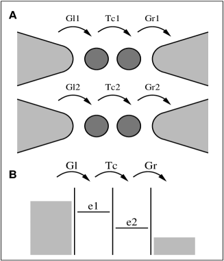
Figure 1: A: $N\!=\!2$ ‘charge qubit register’ with two double quantum dots coupled to independent electron leads. B: energy diagram of one individual double dot.

II.2 Density matrix

In the following, we employ a master equation description for the time evolution of the register within the Born-Markov approximation, which takes into account the interactions with the leads and the bosonic environment up to second order. Alternatively, electron-phonon interactions can be treated exactly by a polaron transformation T. Brandes and B. Kramer, Phys. Rev. Lett. 83, 3021 ; Physica B 272, 42 (1999); Physica B 284-288, 1774(2000) (1999); T. Brandes and T. Vorrath (2002) and perturbatively in the tunnel matrix elements $T_{c,i}$. For $T_{c,i}\lesssim|\varepsilon_{Li}-\varepsilon_{Ri}|$ and small coupling to the bosonic bath, the results of both methods practically coincide T. Brandes, T. Vorrath (2001).

The time derivative of the reduced density matrix $\rho(t)$ of the double quantum dots is given by

$$\begin{split}\dot{\tilde{\rho}}(t)=-\int_{0}^{t}\!dt^{\prime}\;&\Big{(}{\rm Tr}_{\,\textrm{Res,e}}\left\{\big{[}\tilde{H}_{\rm e}(t),\big{[}\tilde{H}_{\rm e}(t^{\prime}),\tilde{\rho}(t)\otimes\tilde{R}_{0,\rm e}\big{]}\big{]}\right\}\\ +&{\rm Tr}_{\,\textrm{Res,\rm p}}\left\{\big{[}\tilde{H}_{\rm p}(t),\big{[}\tilde{H}_{\rm p}(t^{\prime}),\tilde{\rho}(t)\otimes\tilde{R}_{0,\rm p}\big{]}\big{]}\right\}\Big{)},\end{split}$$ (3)

where the tilde indicates the interaction picture, $H_{\rm e}$ ($H_{\rm p}$) denotes the interactions between the double dots and the leads (the phonons), and $R_{0,\rm e}$ ($R_{0,\rm p}$) is the density matrix of the leads (the phonons). Equation (3) is the sum of an electron and a phonon part since we neglect correlations between leads and phonons.

The trace over the equilibrium electron reservoirs, ${\rm Tr}_{\,\textrm{Res,e}}$, results in Fermi functions of the leads. As we are interested in large source-drain voltages between the left and the right leads, the Fermi functions of the left leads can be set to one and those of the right leads to zero. Moreover, the energy dependence of the tunnel rates

$$\Gamma_{L/R,i}=2\pi\sum_{k}|V_{k,i}^{L/R}|^{2}\;\delta(\varepsilon-\varepsilon_{k}^{L/R})$$ (4)

is neglected.

II.2.1 Electron-phonon interaction

In the following, we consider identical electron-phonon interaction in the DQDs,

$$\gamma_{q,i}=\gamma_{q}\,.$$ (5)

Depending on the relative position of the quantum dots (lateral, vertical), the electron wave functions in the dots, and the geometry of the phonon substrate (bulk, slab S. Debald, T. Brandes, B. Kramer (2002), sheet etc.), the $\gamma_{q,i}$ will never be exactly identical in real situations. Therefore, Eq. (5) can only be regarded as an idealized limit of, e.g., a phonon resonator or a situation where the distance between different double dots is small as compared to the relevant phonon wavelengths.

We define a correlation function of the boson system

$$K(t)\equiv\int_{0}^{\infty}\!d\omega\;\rho(\omega)\;\frac{e^{i\omega t}e^{-\beta\omega}+e^{-i\omega t}}{1-e^{-\beta\omega}}\;$$ (6)

that results from the trace over the bosonic degrees of freedom. Here, $\beta=1/k_{B}T$ denotes the inverse phonon bath temperature, and the spectral function $\rho(\omega)$ of the bosonic environment is defined as

$$\rho(\omega)\equiv\sum_{q}|\gamma_{q}|^{2}\;\delta(\omega-\omega_{q}).$$ (7)

For the calculations, we use the spectral function of bulk acoustic phonons with piezoelectric interaction to electrons in lateral quantum dots T. Brandes and B. Kramer, Phys. Rev. Lett. 83, 3021 ; Physica B 272, 42 (1999); Physica B 284-288, 1774(2000) (1999); T. Brandes, T. Vorrath (2001),

$$\rho(\omega)=g\,\omega\,\Big{(}1-\frac{\omega_{d}}{\omega}\sin\Big{(}\frac{\omega}{\omega_{d}}\Big{)}\Big{)}\;e^{-\omega/\omega_{c}},$$ (8)

where $g$ is the dimensionless interaction strength, $\omega_{c}$ the cut-off frequency and the frequency $\omega_{d}$ is determined by the ratio of the the sound velocity to the distance between two quantum dots.

In the following, integrals over $K(t)$ are required as

$$\begin{split}\Gamma_{C,i}&\equiv\int_{0}^{\infty}\!K(t)\,\cos(\Delta_{i}t)\;dt=\frac{\pi}{2}\;\rho(\Delta_{i})\,\coth\!\Big{(}\frac{\beta\Delta_{i}}{2}\Big{)},\\ \Gamma_{S,i}&\equiv\int_{0}^{\infty}\!K(t)\,\sin(\Delta_{i}t)\;dt\,=-i\;\frac{\pi}{2}\;\rho(\Delta_{i}).\end{split}$$ (9)

with the hybridization energy $\Delta_{i}=(\varepsilon_{i}^{2}+4T_{c,i}^{2})^{1/2}$ and the energy bias $\varepsilon_{i}=\varepsilon_{L,i}\!-\!\varepsilon_{R,i}$ in the $i$-th dot. The integrals are calculated neglecting the principal values T. Brandes and T. Vorrath (2002). We furthermore assume a spectral function $\rho(\Delta_{i})$ such that $\Gamma_{C,i}\to 0$ for $\Delta_{i}\to 0$ which is fulfilled for microscopic models of the electron-phonon interaction in double quantum dots T. Brandes and B. Kramer, Phys. Rev. Lett. 83, 3021 ; Physica B 272, 42 (1999); Physica B 284-288, 1774(2000) (1999); T. Brandes and T. Vorrath (2002).

II.2.2 Master equation

Inserting the traces over the electron reservoirs and the bosonic bath into Eq. (3) and transforming back to Schrödinger picture yields a master equation for the reduced density matrix of the total DQD register,

$$\begin{split}&\dot{\rho}(t)=i\;\sum_{i=1}^{N}\Big{\{}\Big{[}\,\rho(t)\,,\varepsilon_{L,i}\,n_{L,i}+\varepsilon_{R,i}\,n_{R,i}+T_{c,i}(p_{i}+p_{i}^{\dagger})\Big{]}\\ &+\frac{\Gamma_{L,i}}{2}\Big{(}2\,s_{L,i}^{\dagger}\,\rho(t)\,s_{L,i}-\,s_{L,i}\,s_{L,i}^{\dagger}\,\rho(t)-\,\rho(t)\,s_{L,i}\,s_{L,i}^{\dagger}\Big{)}\\ &+\frac{\Gamma_{R,i}}{2}\Big{(}2\,s_{R,i}\,\rho(t)\,s_{R,i}^{\dagger}-s_{R,i}^{\dagger}\,s_{R,i}\,\rho(t)-\rho(t)\,s_{R,i}^{\dagger}\,s_{R,i}\Big{)}\Big{\}}\\ &-\sum_{i,j}\,\Big{\{}\Big{[}(n_{L,i}\!-\!n_{R,i}),A_{j}\,\rho(t)\Big{]}\!-\!\Big{[}(n_{L,i}\!-\!n_{R,i}),\rho(t)A_{j}^{\dagger}\Big{]}\Big{\}},\end{split}$$ (10)

with

$$\begin{split}A_{j}&\equiv\frac{2T_{c,j}}{\Delta_{i}^{2}}\,\Big{(}\,2T_{c,j}\Gamma_{C,j}(n_{L,j}\!-\!n_{R,j})\\ &-\Gamma_{C,j}\,\varepsilon_{j}\,(p_{j}+p_{j}^{\dagger})+i\,\Delta_{j}\Gamma_{S,j}(p_{j}-p_{j}^{\dagger})\,\Big{)}.\end{split}$$ (11)

From Eq. (9) it is obvious that the influence of the bosonic bath enters only via the spectral functions $\rho(\omega)$ as defined in Eq. (7). All microscopic properties of the phonons and their interaction mechanism to the electrons in the quantum dots are described by these functions.

Furthermore, we point out that the mixed terms $i\not=j$ in Eq. (10) are responsible for the collective effects to be discussed in the following. Without these terms, the master equation would merely describe an ensemble of $N$ independent DQDs. In that case, an initially factorized density matrix of the total system would always remain factorized and no correlations could build up. The terms $i\not=j$ introduce correlations between the different double dots, the origin of which lies in the coupling to the same bosonic environment.

III Current superradiance

We restrict ourselves to the stationary case where the time derivative of the density matrix, $\dot{\rho}(t)$, vanishes. Then, Eq. (10) reduces to a linear system of equations which can be easily solved numerically. Results for a single double quantum dot, $N\!=\!1$, can be obtained analytically T. Brandes, T. Vorrath (2001) and are given for two expectation values below, Eq. (17). For $N>1$, the dimension of the density matrix grows as $9^{N}$ (although not all of the matrix elements are required) whence analytical solutions become very cumbersome. For the rest of this paper, we restrict ourselves to the case of two double dots ($N=2$), called DQD 1 and DQD 2 in the following.

III.1 Stationary current

The total electron current is simply given by the sum of the currents through the individual DQDs, as electrons cannot tunnel between different double dots. The current operator of DQD $i$ is

$$I_{i}=\frac{i\,T_{c,i}\,e}{\hbar}\;(p_{i}-p_{i}^{\dagger}),$$ (12)

and the corresponding expectation values can be expressed by the elements of the density matrix as

$$\begin{split}I_{1}&=-\,\frac{2\,T_{c,1}\,e}{\hbar}\;\;\mbox{Im}\big{\{}\rho_{LRLL}+\rho_{RRLR}+\rho_{0RL0}\big{\}},\\ I_{2}&=-\,\frac{2\,T_{c,2}\,e}{\hbar}\;\;\mbox{Im}\big{\{}\rho_{RLLL}+\rho_{RRRL}+\rho_{R00L}\big{\}},\end{split}$$ (13)

with the notation

$$\rho_{j\,i\,i^{\prime}\,j^{\prime}}=\;{}_{2}\!\left\langle j\right|\otimes{}_{1}\!\left\langle i\right|\,\rho\,\left|i^{\prime}\right\rangle_{1}\otimes\left|j^{\prime}\right\rangle_{2},\quad i,j\in\{L,R,0\}.$$ (14)

The set of linear equations corresponding to Eq. (10) for $N\!=\!2$ is given in appendix A, Eq. (32).

Figure 2: Total current through two double quantum dots as a function of the bias $\varepsilon_{1}$. The parameters are $T_{c,1}\!=\!T_{c,2}\!=\!3\mu$eV, $\Gamma_{L,1}\!=\!\Gamma_{R,1}\!=\!\Gamma_{L,2}\!=\!\Gamma_{R,2}\!=\!0.15\mu$eV, and for the spectral function $g\!=\!0.01$, $T\!=\!23$mK, $\omega_{d}\!=\!10\mu$eV and $\omega_{c}\!=\!1$meV. These values are used throughout the whole article if not stated otherwise.

From the numerical solution of Eq. (32) we find the stationary current through two double quantum dots as a function of the bias $\varepsilon_{1}$ in the first double dot while the bias $\varepsilon_{2}$ in the second is kept constant, cf. Fig. 2. The overall shape of the current is very similar to the case of one individual double quantum dot T. Brandes and B. Kramer, Phys. Rev. Lett. 83, 3021 ; Physica B 272, 42 (1999); Physica B 284-288, 1774(2000) (1999); T. Brandes, T. Vorrath (2001), with its strong elastic peak around $\varepsilon_{1}=0$ and a broad inelastic shoulder for $\varepsilon_{1}>0$. The interesting new feature here is the peak at the resonance $\varepsilon_{1}\!=\!\varepsilon_{2}$ which is due to collective effects to be analyzed now.

III.2 Cross coherences

The effective interaction between the two DQDs results from the simultaneous coupling of both double dots to the same phonon environment. It appears in the master equation (10) as the mixed terms $i\!\neq\!j$ in the sum. In the explicit form of the master equation (32), the effective interaction is connected to six matrix elements only (and their complex conjugates). These elements are $\rho_{RLLL}$, $\rho_{LRLL}$, $\rho_{RRLR}$ and $\rho_{RRRL}$, all of which enter the expression for the current, Eq. (13), and the two ‘cross coherence’ matrix elements

$$\rho_{RLRL}=\big{\langle}p_{1}^{\dagger}p_{2}\big{\rangle},\quad\rho_{RRLL}=\big{\langle}p_{1}p_{2}\big{\rangle}.$$ (15)

Therefore, we approximate the collective effects caused by the effective interaction starting from the solution of the non-interacting master equation, without the mixed terms $i\!\neq\!j$, and assume that only those matrix elements mentioned above are affected by the interaction.

In the non-interacting case, the cross coherence is simply the product of the corresponding matrix elements of independent double dots,

$$\big{\langle}p_{1}^{\dagger}p_{2}\big{\rangle}=\big{\langle}p_{1}^{\dagger}\big{\rangle}\left\langle p_{2}\right\rangle,\quad\big{\langle}p_{1}p_{2}\big{\rangle}=\left\langle p_{1}\right\rangle\left\langle p_{2}\right\rangle.$$ (16)

These can be solved analytically,

$$\begin{split}\left\langle p_{j}\right\rangle&=-\frac{\Gamma_{L,j}}{M_{j}}\Big{(}2T_{c,j}^{2}(\beta_{j}+\gamma_{j})\\ &+\Gamma_{R,j}(iT_{c,j}+\gamma_{j})(i\varepsilon_{j}+\frac{1}{2}\Gamma_{R,j}+2\alpha_{j})\Big{)},\\ \left\langle n_{L,j}\right\rangle&=1-\frac{T_{c,j}(\Gamma_{L,j}\!+\!\Gamma_{R,j})}{M_{j}}\Big{(}2\varepsilon_{j}\gamma_{j}+T_{c,j}(\Gamma_{R,j}+4\alpha_{j})\Big{)},\end{split}$$ (17)

where $\left\langle n_{L,j}\right\rangle$ is given for later reference, $\alpha_{j}$, $\beta_{j}$, and $\gamma_{j}$ as defined in the appendix, Eq. (34), and with

$$\begin{split}&M_{j}\equiv\Gamma_{L,j}\Gamma_{R,j}\Big{(}\varepsilon_{j}^{2}+\Big{(}\frac{1}{2}\Gamma_{R,j}\!+\!2\alpha_{j}\Big{)}^{2}\,\Big{)}-2T_{c,j}\varepsilon_{j}\beta_{j}\Gamma_{L,j}\\ &+T_{c,j}^{2}(2\Gamma_{L,j}\!+\!\Gamma_{R,j})(\Gamma_{R,j}\!+\!4\alpha_{j})+2T_{c,j}\varepsilon_{j}\gamma_{j}(\Gamma_{L,j}\!+\!\Gamma_{R,j}).\end{split}$$ (18)

In the inelastic regime, $T_{c}\!\ll\!\varepsilon$, of the non-interacting case, the cross coherences $\big{\langle}p_{1}^{\dagger}p_{2}\big{\rangle}$ and $\big{\langle}p_{1}p_{2}\big{\rangle}$ tend to zero as can be seen from Eq. (17). Moreover, we neglect the imaginary part of the cross coherences in the interacting case. Then, the change in the current through DQD 1 due to collective effects can be approximated by

$$\Delta I_{1}=\frac{2e\,T_{c,1}\,\gamma_{2}}{\hbar\,\varepsilon_{1}}\,\Big{(}\textrm{Re}\Big{\{}\big{\langle}p_{1}^{\dagger}p_{2}\big{\rangle}\Big{\}}-\textrm{Re}\Big{\{}\big{\langle}p_{1}p_{2}\big{\rangle}\Big{\}}\Big{)}.$$ (19)

Correspondingly, the change $\Delta I_{2}$ of the current through the second double dot DQD 2 is obtained from $\Delta I_{1}$ by exchanging the subscripts 1 and 2. Hence, the alteration in the current is proportional to the real parts of the cross coherences $\big{\langle}p_{1}^{\dagger}p_{2}\big{\rangle}$ and $\big{\langle}p_{1}p_{2}\big{\rangle}$ between the two DQDs, which confirms the collective character of the effect. This result is corroborated by plotting the real parts of the cross coherences as a function of $\varepsilon_{1}$, cf. Fig. 3. One recognizes that $\big{\langle}p_{1}^{\dagger}p_{2}\big{\rangle}$ is peaked around $\varepsilon_{1}\!=\!\varepsilon_{2}$, whereas $\big{\langle}p_{1}p_{2}\big{\rangle}$ has a peak at $\varepsilon_{1}\!=\!-\varepsilon_{2}$. The increase of the current at $\varepsilon_{1}\!=\!\varepsilon_{2}$ is therefore due to the maximum of the first correlation $\big{\langle}p_{1}^{\dagger}p_{2}\big{\rangle}$.

If we neglect the changes of all other elements of the density matrix that are caused by the effective interaction between the two DQDs, the real part of the cross coherence $\big{\langle}p_{1}^{\dagger}p_{2}\big{\rangle}$ can be approximated around the resonance $\varepsilon_{1}\!=\!\varepsilon_{2}$ as

$$\begin{split}\textrm{Re}\Big{\{}\big{\langle}p_{1}^{\dagger}p_{2}\big{\rangle}\Big{\}}&=\frac{\frac{1}{2}\,(\Gamma_{R,1}+\Gamma_{R,2})}{(\varepsilon_{1}\!-\!\varepsilon_{2})^{2}+\frac{1}{4}(\Gamma_{R,1}+\Gamma_{R,2})^{2}}\cdot\\ &\Big{(}\gamma_{1}\,\textrm{Re}\big{\{}\!\left\langle p_{2}\right\rangle\!\big{\}}\left\langle n_{L,1}\right\rangle+\gamma_{2}\,\textrm{Re}\big{\{}\!\left\langle p_{1}\right\rangle\!\big{\}}\left\langle n_{L,2}\right\rangle\Big{)}.\end{split}$$ (20)

One recognizes that $\big{\langle}p_{1}^{\dagger}p_{2}\big{\rangle}$ is Lorentzian shaped as a function of the energy difference $\varepsilon_{1}\!-\!\varepsilon_{2}$. The result of Eq. (20) with $\left\langle p_{j}\right\rangle$ and $\left\langle n_{L,j}\right\rangle$ as given in Eq. (17) is in good agreement with the numerical solution of the master equation (10) (inset of Fig. 3).

Next, we insert the result for the cross coherence in Eq. (19) and find for the change of the tunnel current due to interaction effects between the two double quantum dots around the resonance $\varepsilon_{1}\!=\!\varepsilon_{2}$:

$$\begin{split}\Delta I_{1}=\,&\frac{e\,T_{c,1}\,\gamma_{2}}{\hbar\,\varepsilon_{1}}\,\frac{\Gamma_{R,1}\!+\!\Gamma_{R,2}}{(\varepsilon_{1}\!-\!\varepsilon_{2})^{2}+\frac{1}{4}(\Gamma_{R,1}\!+\!\Gamma_{R,2})^{2}}\cdot\\ &\Big{(}\gamma_{1}\,\textrm{Re}\big{\{}\!\left\langle p_{2}\right\rangle\!\big{\}}\left\langle n_{L,1}\right\rangle+\gamma_{2}\,\textrm{Re}\big{\{}\!\left\langle p_{1}\right\rangle\!\big{\}}\left\langle n_{L,2}\right\rangle\Big{)}.\end{split}$$ (21)

Again, the change in the current through the second double dot, $\Delta I_{2}$, is obtained by exchanging the subscripts. This approximation overestimates the actual change in the current for the parameters chosen in the previous section but provides a good qualitative description for the effect of the enhanced tunnel current. A comparison between this result and the numerical solution is given below.

Figure 3: Real parts of the cross coherences from the master equation (10) as functions of the bias in the first double dot ($\varepsilon_{2}\!=\!30\mu$eV and the other parameters agree with Fig. 2). The inset compares the approximation for $\textrm{Re}\big{\{}\big{\langle}p_{1}^{\dagger}p_{2}\big{\rangle}\big{\}}$, Eq. (20) (dotted line), with the solution of the master eq. (solid line).

III.3 Singlet and triplet states

The collective effects in the two double quantum dots are connected with the cross coherence function $\big{\langle}p_{1}^{\dagger}p_{2}\big{\rangle}$, Eq. (15). For the ‘two-qubit register’ one can easily prove the operator identity

$$p_{1}^{\dagger}p_{2}+p_{2}^{\dagger}p_{1}=\textrm{P}_{T_{0}}-\textrm{P}_{S_{0}},$$ (22)

where $\textrm{P}_{\psi}$ is the projection operator on the state $\left|\psi\right\rangle$, $\textrm{P}_{\psi}\equiv\left|\psi\right\rangle\left\langle\psi\right|$, and triplet and singlet do not refer to the real electron spin but to the ‘pseudo’ spin defined in the two dimensional Hilbert space ${\rm span}(|L\rangle,|R\rangle)$,

$$\begin{split}\left|T_{+}\right\rangle&=\left|L\right\rangle_{1}\left|L\right\rangle_{2},\quad\left|T_{-}\right\rangle=\left|R\right\rangle_{1}\left|R\right\rangle_{2},\\ \left|T_{0}\right\rangle&=\frac{1}{\sqrt{2}}\,\Big{(}\left|L\right\rangle_{1}\left|R\right\rangle_{2}+\left|R\right\rangle_{1}\left|L\right\rangle_{2}\Big{)},\\ \left|S_{0}\right\rangle&=\frac{1}{\sqrt{2}}\,\Big{(}\left|L\right\rangle_{1}\left|R\right\rangle_{2}-\left|R\right\rangle_{1}\left|L\right\rangle_{2}\Big{)}.\end{split}$$ (23)

With $2\,\textrm{Re}\big{\langle}p_{1}^{\dagger}p_{2}\big{\rangle}=\big{\langle}\textrm{P}_{T_{0}}\big{\rangle}-\big{\langle}\textrm{P}_{S_{0}}\big{\rangle}$ and the proportionality $\Delta I_{1}\propto\textrm{Re}\big{\langle}p_{1}^{\dagger}p_{2}\big{\rangle}$ for $\varepsilon_{1}\approx\varepsilon_{2}$, cf. Eq. (19), it follows that the current enhancement $\Delta I_{1}$ is due to an increased probability of finding the two electrons in a (pseudo) triplet rather than in a (pseudo) singlet state. In the following, we demonstrate that the mechanism underlying this effect is indeed the Dicke superradiance effect known from quantum optics.

III.4 Dicke effect

Superradiance emerges in the collective spontaneous emission from an ensemble of identical two-level atoms. If $N$ excited atoms are concentrated in a region smaller than the wavelength of the emitted radiation, they do not decay independently anymore. Instead, the radiation has a higher intensity and takes place in a shorter time interval than for an ensemble of independent atoms due to the coupling of all atoms to the common radiation field.

Let us now consider the case $N\!=\!2$ and calculate (similar to the original work of Dicke Dicke (1954)) the decay rate $\Gamma$ of two initially excited atoms with dipole moments $\hat{{d}}_{1}$ and $\hat{{d}}_{2}$) at position ${\bf r}_{1}$ and ${\bf r}_{2}$ due to the interaction with light,

$$\begin{split}H_{eph}&=\sum_{{\bf Q}}{{g}}_{{\bf Q}}\left(a_{-{\bf Q}}+a_{{\bf Q}}^{+}\right)\\ &\times\left[\hat{{d}}_{1}\exp{i({\bf Qr}_{1})}+\hat{{d}}_{2}\exp{i({\bf Qr}_{2})}\right],\end{split}$$ (24)

from which the spontaneous emission rate of photons with wave vector ${\bf Q}$ follows (Fermi’s Golden Rule),

$$\Gamma_{\pm}(Q)\propto\!\sum_{{\bf Q}}|g_{Q}|^{2}{|1\pm\exp{[i{\bf Q}({\bf r}_{2}-{\bf r}_{1})]}|^{2}}\delta(\omega_{0}-\omega_{Q}),$$ (25)

where $Q=\omega_{0}/c$, $\omega_{0}$ is the transition frequency between the upper and lower level, and $c$ denotes the speed of light. The interference of the two interaction contributions $\hat{{d}}_{1}e^{i({\bf Qr}_{1})}$ and $\hat{{d}}_{2}e^{i({\bf Qr}_{2})}$ leads to a splitting of the spontaneous decay into a fast, ‘superradiant’, decay channel ($\Gamma_{+}(Q)$), and a slow, ‘subradiant’ decay channel ($\Gamma_{-}(Q)$). This splitting is called ‘Dicke-effect’.

Loosely speaking, the two signs $\pm$ correspond to the two different relative orientations of the dipole moments of the two atoms. More precisely, from the four possible states in the Hilbert space of two two–level systems, ${\cal{H}}_{2}=C^{2}\otimes C^{2}$, one can form singlet and triplet states according to $|S_{0}\rangle:=\frac{1}{\sqrt{2}}\left(|\uparrow\downarrow\rangle-|\downarrow\uparrow\rangle\right)$, $|T_{+}\rangle:=|\uparrow\uparrow\rangle$, $|T_{0}\rangle:=\frac{1}{\sqrt{2}}\left(|\uparrow\downarrow\rangle+|\downarrow\uparrow\rangle\right)$, and $|T_{-}\rangle:=|\downarrow\downarrow\rangle$. The superradiant decay channel occurs via the triplet and the subradiant decay via the singlet states Dicke (1954); M. Gross, S. Haroche (1982). In the extreme ‘Dicke’ limit where the second phase factor is close to unity, $\exp{[i{\bf Q}({\bf r}_{2}-{\bf r}_{1})]}\approx 1$, it follows that $\Gamma_{-}(Q)=0$ and $\Gamma_{+}(Q)=2\Gamma(Q)$ where $\Gamma(Q)$ is the decay rate of one single atom. This limit is theoretically achieved if $|{\bf Q}({\bf r}_{2}-{\bf r}_{1})|\ll 1$ for all wave vectors ${\bf Q}$, i.e. the distance between the two atoms is much smaller than the wave length of the light.

We mention that in practice, this ‘pure’ limit, where the subradiant rate is zero and the superradiant rate is just twice the rate for an individual atom, is never reached. In a recent experimental realization of sub- and superradiance from two laser-trapped ions, DeVoe and Brewer DeVoe and Brewer (1996) measured the spontaneous emission rate of photons as a function of the ion-ion distance in a laser trap of planar geometry which was strong enough to bring the ions (Ba${}_{138}^{+}$) to a distance of the order of 1$\mu$m of each other.

The two double quantum dots behave in analogy to the two atoms considered above. For a positive bias, $\varepsilon\!=\!\varepsilon_{L}\!-\!\varepsilon_{R}\!>\!0$, the state $\left|L\right\rangle$ can be identified with the excited state and $\left|R\right\rangle$ with the ground state. The inelastic rate $\nu$ with which $\left|L\right\rangle$ decays to $\left|R\right\rangle$ can be calculated with Fermi’s Golden Rule,

$$\nu=\frac{8\,\pi\,T_{c}^{2}}{\hbar\,(\varepsilon^{2}\!+\!4T_{c}^{2})}\;\rho\big{(}\sqrt{\varepsilon^{2}\!+\!4T_{c}^{2}}\,\big{)}.$$ (26)

In contrast to a two level atom, a third state $\left|0\right\rangle$ exists in the double quantum dot as the additional electron can tunnel into the leads.

The use of triplet and singlet states as defined in Eq. (23) allows us to find an analytical result for the stationary current that quantitatively coincides with the exact numerical solution extremely well. We consider the rate equation for the probabilities of the corresponding nine states and take into account the doubling of the inelastic rates due to the Dicke effect in the triplet channel,

$$\begin{split}\dot{p}_{00}&=\Gamma\,p_{R0}+\Gamma\,p_{0R}-2\Gamma\,p_{00},\\ \dot{p}_{L0}&=\Gamma\,p_{00}+\frac{1}{2}\,\Gamma\,p_{T_{0}}+\frac{1}{2}\,\Gamma\,p_{S_{0}}-(\nu+\Gamma)\,p_{L0},\\ \dot{p}_{0L}&=\Gamma\,p_{00}+\frac{1}{2}\,\Gamma\,p_{T_{0}}+\frac{1}{2}\,\Gamma\,p_{S_{0}}-(\nu+\Gamma)\,p_{0L},\\ \dot{p}_{R0}&=\nu\,p_{L0}+\Gamma\,p_{T-}-2\Gamma\,p_{R0},\\ \dot{p}_{0R}&=\nu\,p_{0L}+\Gamma\,p_{T-}-2\Gamma\,p_{0R},\\ \dot{p}_{T+}&=\Gamma\,p_{0L}+\Gamma\,p_{L0}-2\nu\,p_{T+},\\ \dot{p}_{T_{0}}&=2\nu\,p_{T+}+\frac{1}{2}\,\Gamma\,p_{0R}+\frac{1}{2}\,\Gamma\,p_{R0}-(2\nu+\Gamma)\,p_{T_{0}},\\ \dot{p}_{T-}&=2\nu\,p_{T_{0}}-2\Gamma\,p_{T-},\\ \dot{p}_{S_{0}}&=\frac{1}{2}\,\Gamma\,p_{0R}+\frac{1}{2}\,\Gamma\,p_{R0}-\Gamma\,p_{S_{0}}.\end{split}$$ (27)

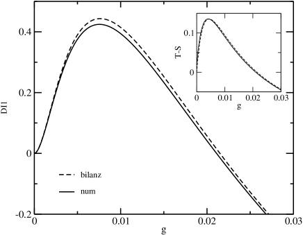
Figure 4: Enhancement of the tunnel current $\Delta I_{1}$ at the resonance $\varepsilon_{1}\!=\!\varepsilon_{2}\!=\!30\mu$eV as a function of the dimensionless electron phonon coupling constant $g$, Eq. (8). The additional current vanishes at $g\!\approx\!0.02$ when the tunnel rates to the double dot and between the dots become equal, $\nu\!=\!\Gamma$. The inset shows the difference in probabilities for triplet and singlet.

Here, identical tunnel rates to all four leads have been assumed, $\Gamma_{L,1}\!=\!\Gamma_{R,1}\!=\!\Gamma_{L,2}\!=\!\Gamma_{R,2}\!=\!\Gamma$, and $p_{L0}$ denotes the probability to find the first double dot in state $\left|L\right\rangle$ and the second in state $\left|0\right\rangle$. Electrons can also tunnel into and out of the singlet state due to the coupling to the leads which is not possible in the original Dicke model. In the stationary case, the Eq. (27) can be easily solved. For the current through one of the two double dots we obtain

$$\begin{split}I_{1}&=\frac{e\,\Gamma}{\hbar}\;(p_{00}+p_{0L}+p_{0R})\\ &=\frac{e\,\Gamma}{\hbar}\;\frac{x(4x+1)}{9x^{2}+5x+1},\quad x=\nu/\Gamma.\end{split}$$ (28)

This can be compared with the tunnel current through one independent double dot, $I_{1}^{0}$ obtained by a similar rate equation,

$$I_{1}^{0}=\frac{e\,\Gamma}{\hbar}\;\frac{x}{1+2x}.$$ (29)

The difference $\Delta I_{1}=I_{1}-I_{1}^{0}$ represents the additional current due to the Dicke effect and is shown in Fig. 4 as a function of the dimensionless coupling strength $g$ to the bosonic environment, together with a comparison to the $\Delta I_{1}$ as obtained from the numerical solution of Eq. (10). Both results agree very well, indicating that it is indeed the Dicke effect that leads to the increase in the tunnel current. In addition, we show (inset of Fig. 4) the difference between triplet and singlet occupation probability that follow from the Eq. (27) as

$$p_{T_{0}}-p_{S_{0}}=-\frac{2x(x+2)(x-1)}{9x^{3}+23x^{2}+11x+2}.$$ (30)

This is in excellent agreement with the numerical results and underlines that the change in the tunnel current due to collective effects is proportional to $p_{T_{0}}-p_{S_{0}}$, as already discussed above. This demonstrates that the effect of superradiance amplifies the tunneling of electrons from the left to the right dots resulting in an enhanced current through the two double quantum dots.

IV Current subradiance and inelastic switch

The close analogy with the Dicke effect suggests the existence of not only current super-, but also current subradiance in the register. In the subradiant regime, the two DQDs form a singlet state where the tunneling from the left to the right quantum dots is diminished, resulting in a weaker tunnel current through the dots.

IV.1 Current antiresonance

Subradiance occurs in our system in a slightly changed set-up where electrons in the second double dot are prevented from tunneling into the right lead, $\Gamma_{R,2}\!=\!0$, as indicated in the inset of Fig. 5. Then, the additional electron is trapped and no current can flow through the second double dot. Nevertheless, this electron can affect the tunnel current through the first double dot: Instead of a maximum, we now find a minimum at the resonance $\varepsilon_{1}\!=\!\varepsilon_{2}$. Fig. 5 shows how the positive peak in the current $I_{1}$ develops into a minimum as the tunneling rate $\Gamma_{R,2}$ is decreased to zero. This minimum is indeed related to an increased probability of finding the two dots in the singlet state $\left|S_{0}\right\rangle$ rather than in the triplet state $\left|T_{0}\right\rangle$, as can be seen from the inset of Fig. 5. Thus, in this regime the effect of subradiance dominates, leading to a decreased current.

This behavior is again consistent with the approximation Eq. (20) for the cross coherence $\big{\langle}p_{1}^{\dagger}p_{2}\big{\rangle}$. Taking into account the different non-interacting matrix elements in the two double dots, $\left\langle n_{L,1}\right\rangle\!\neq\!\left\langle n_{L,2}\right\rangle$ and $\left\langle p_{1}\right\rangle\!\neq\!\left\langle p_{2}\right\rangle$ due to $\Gamma_{R,1}\!\neq\!\Gamma_{R,2}$, we find a negative cross coherence at the resonance from Eq. (20). This corresponds to an increased probability for the singlet state and according to Eq. (21) to a negative peak in the tunnel current, in agreement with our numerical solution.

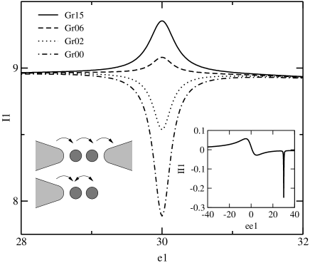
Figure 5: Transition from an increased to a decreased current through the first double quantum dot for different tunnel rates $\Gamma_{R,2}$ (in $\mu$eV) and $\varepsilon_{2}\!=\!30\mu$eV. The left inset shows schematically the set-up for $\Gamma_{R,2}\!=\!0$ and the right inset gives the difference of triplet and singlet for the same case.

IV.2 Inelastic current switch

Up to now, we have regarded the cross coherence $\big{\langle}p_{1}^{\dagger}p_{2}\big{\rangle}$ and its effects on the current only at the resonance $\varepsilon_{1}\!=\!\varepsilon_{2}$. However, it was already pointed out in section III.2 that another cross coherence, $\big{\langle}p_{1}p_{2}\big{\rangle}$, exhibits a resonance if the bias in one dot equals the negative bias in the other dot, $\varepsilon_{1}\!=\!-\varepsilon_{2}$ (cp. Fig. 3). This case is considered in the following.

We use a fixed negative bias $\varepsilon_{2}\!<\!0$ in the second double dot as indicated in the inset of Fig. 6. Consequently, electrons cannot tunnel from the left to the right dot such that the second double dot is blocked and no current can flow through it. The presence of the first double dot, though, lifts this blockade and enables a current through the second double dot if the resonance condition $\varepsilon_{1}\!=\!-\varepsilon_{2}$ is fulfilled. The current $I_{2}$ is shown in Fig. 6 as a function of the bias in the first double dot, $\varepsilon_{1}$. Due to the coupling to the common phonon environment, energy is transferred from the first to the second double dot, allowing electrons to tunnel from the left to the right in the second double dot. At the same time, the current through the first double dot is decreased (not shown here).

We can approximate the current through the second double dot around $\varepsilon_{1}\!=\!-\varepsilon_{2}$ taking into account only $\big{\langle}p_{1}p_{2}\big{\rangle}$ in Eq. (19). A similar calculation as for $\big{\langle}p_{1}^{\dagger}p_{2}\big{\rangle}$, Eq. (20), gives

$$\begin{split}\Delta I_{2}=\frac{2T_{c,2}\,\gamma_{1}\,e}{\varepsilon_{2}\,\hbar}\;\frac{\frac{1}{2}\Gamma_{R,1}\!+\!\frac{1}{2}\Gamma_{R,2}\!+\!8\alpha}{(\varepsilon_{1}\!+\!\varepsilon_{2})^{2}+(\frac{1}{2}\Gamma_{R,1}\!+\!\frac{1}{2}\Gamma_{R,2}\!+\!8\alpha)^{2}}\\ \Big{(}\gamma_{1}\,\textrm{Re}\big{\{}\!\left\langle p_{2}\right\rangle\!\big{\}}\,\left\langle n_{L,1}\right\rangle+\gamma_{2}\,\textrm{Re}\big{\{}\!\left\langle p_{1}\right\rangle\!\big{\}}\,\left\langle n_{L,2}\right\rangle\Big{)},\end{split}$$ (31)

with $\alpha\!=\!\alpha_{1}\!=\!\alpha_{2}$ evaluated at the resonance, where both systems are identical except of the bias. This approximation again is in good agreement with the numerical solution of Eq. (10), as can be seen from Fig. 6.

Our results suggest that the current through one of the DQDs can be switched on and off by appropriate manipulation of the other one. We emphasize that this mechanism is mediated by the dissipative phonon environment and not the Coulomb interaction between the charges. As this effect is very sensitive to the energy bias, it allows to detect a certain energy bias in one double dot by observing the current through the other double dot.

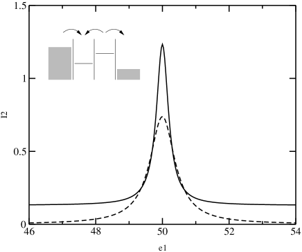
Figure 6: Tunnel current through the second double dot which is blocked due to a negative bias, $\varepsilon_{2}\!=\!-50\mu$eV, as depicted in the inset ($g\!=\!0.015$). The approximation for $\Delta I_{2}$, Eq. (31) (dashed line), agrees well with the result of the master equation (10) (solid line – the finite offset of which is the tail of the elastic current at $\varepsilon_{2}\!=\!0$).

V Conclusion

In this work, we have investigated collective effects in two double quantum dots. An indirect interaction arises between the two double dots due to the coupling to the same phonon environment. We predict that the Dicke effect causes a considerable increase or decrease of the tunnel current, depending on the choice of the parameters. The occurrence of the Dicke effect in the transport through mesoscopic systems has already been pointed out by Shahbazyan and Raikh Shahbazyan and Raikh (1994). In their system, the coupling to the same lead is responsible for collective effects. Usually, the Dicke effect manifests itself in a dynamic process like the spontaneous emission of an ensemble of identical atoms DeVoe and Brewer (1996); Greiner_00 . Transport through double quantum dots, however, allows to study a time independent form of the Dicke effect. Moreover, we have demonstrated that the change of the tunnel current is connected with an entanglement of the different double dots. This opens the possibility to realize and to measure specific entangled states of two double dots. In particular, one can switch from a predominant triplet superposition of the two double dots connected with an increased tunnel current to a predominate singlet state leading to a reduced current.

The results discussed here were derived for the ideal case of an identical electron-phonon coupling in both double quantum dots. Furthermore, the Coulomb interaction between the two double dots has not been considered here. In a real experiment, these assumption will never be perfectly fulfilled and would lead to deviations from the collective effects presented above. However, we predict that even in presence of inter-dot Coulomb interactions, phonon mediated collective effects should persist as long as a description of the register in terms of few many-body states is possible. These many-body states (that would depend on the specific geometry of the register) would than replace the many-body basis $\{|0,i\rangle,|L,i\rangle,|R,i\rangle\}$ ($i=1,2$) used in our model here.

We have derived the master equation for the general case of $N$ double dots but only focused on $N=2$ which is the simplest case where collective effects occur. In general, one of the main characteristic features of superradiance is the quadratic increase of the effect with increasing number of coupled systems. For the spontaneous collective emission from $N$ excited two level atoms, this means that the maximum of the intensity of the emitted radiation increases with the square number of systems, $N^{2}$, while the time in which the decay takes place decreases inversely to the number of systems, $1/N$. Therefore, we expect that the collective effects as presented here become even more pronounced if more than two double dots are indirectly coupled by the common phonons.

Appendix A Master Equation for two double quantum dots

The dimension of the density matrix $\rho$ for $N$ double quantum dots is equal to $9^{N}$ such that the master equation (10) corresponds to 81 coupled differential equations for $N\!=\!2$. It is, however, not necessary to solve all 81 equations as we study the current which requires the knowledge of only six matrix elements, cp. Eq. (13). The smallest closed subset of equations, containing the equations for those six elements consists of 25 equations.

The mixed terms in the master equation (10), $i\neq j$, describing the indirect interaction between the two DQDs due to the coupling to the same phonons, are marked in the following with an additional prefactor $q$. Setting $q\!=\!0$ results in the master equation for two completely independent double dots coupled to independent phonons. The interacting case corresponds to $q\!=\!1$. Note that the elements of the density matrix are expressed with respect to the basis $\{$$\left|L\right\rangle,\left|R\right\rangle,\left|0\right\rangle$$\}$ for each double dot. Due to the tunneling of electrons between the left and right quantum dot, these states are no eigenstates of the unperturbed Hamiltonian. Finally, the master equation for the elements of the density matrix reads

$$\begin{split}\dot{\rho}_{LLLL}&=iT_{c,1}(\rho_{LLRL}-\rho_{LRLL})+iT_{c,2}(\rho_{LLLR}-\rho_{RLLL})+\Gamma_{L,1}\,\rho_{L00L}+\Gamma_{L,2}\,\rho_{0LL0},\\ \dot{\rho}_{LLLR}&=iT_{c,1}(\rho_{LLRR}-\rho_{LRLR})+iT_{c,2}(\rho_{LLLL}-\rho_{RLLR})+\Gamma_{L,1}\,\rho_{L00R}-\gamma_{2}\,\rho_{LLLL}-\beta_{2}\,\rho_{RLLR}\\ &-\big{(}i\varepsilon_{2}+\frac{1}{2}\Gamma_{R,2}+2\alpha_{2}\big{)}\,\rho_{LLLR}+q\,\beta_{1}\big{(}\rho_{LLRR}-\rho_{LRLR}\big{)},\\ \dot{\rho}_{LLRL}&=iT_{c,1}(\rho_{LLLL}-\rho_{LRRL})+iT_{c,2}(\rho_{LLRR}-\rho_{RLRL})+\Gamma_{L,2}\,\rho_{0LR0}-\gamma_{1}\,\rho_{LLLL}-\beta_{1}\,\rho_{LRRL}\\ &-\big{(}i\varepsilon_{1}+\frac{1}{2}\Gamma_{R,1}+2\alpha_{1}\big{)}\,\rho_{LLRL}+q\,\beta_{2}\big{(}\rho_{LLRR}-\rho_{RLRL}\big{)},\\ \dot{\rho}_{LLRR}&=iT_{c,1}(\rho_{LLLR}-\rho_{LRRR})+iT_{c,2}(\rho_{LLRL}-\rho_{RLRR})-\gamma_{1}\,\rho_{LLLR}-\beta_{1}\,\rho_{LRRR}\\ &-\gamma_{2}\,\rho_{LLRL}-\beta_{2}\,\rho_{RLRR}-\big{(}i\varepsilon_{1}+i\varepsilon_{2}+\frac{1}{2}\Gamma_{R,1}+\frac{1}{2}\Gamma_{R,2}+2\alpha_{1}+2\alpha_{2}\big{)}\,\rho_{LLRR}\\ &-q\;\big{(}\!2(\alpha_{1}\!+\!\alpha_{2})\,\rho_{LLRR}+\beta_{2}\,\rho_{RLRR}+\beta_{1}\,\rho_{LRRR}+\gamma_{2}\,\rho_{LLRL}+\gamma_{1}\,\rho_{LLLR}\big{)},\\ \dot{\rho}_{RLLR}&=iT_{c,1}(\rho_{RLRR}-\rho_{RRLR})+iT_{c,2}(\rho_{RLLL}-\rho_{LLLR})+\Gamma_{L,1}\,\rho_{R00R}-\Gamma_{R,2}\,\rho_{RLLR},\\ \dot{\rho}_{RLRL}&=iT_{c,1}(\rho_{RLLL}-\rho_{RRRL})+iT_{c,2}(\rho_{RLRR}-\rho_{LLRL})-\gamma_{1}\,\rho_{RLLL}-\beta_{1}\,\rho_{RRRL}\\ &-\gamma_{2}\,\rho_{LLRL}-\beta_{2}\,\rho_{RLRR}-\big{(}i\varepsilon_{1}\!-i\varepsilon_{2}+\frac{1}{2}\Gamma_{R,1}+\frac{1}{2}\Gamma_{R,2}+2\alpha_{1}+2\alpha_{2}\big{)}\,\rho_{RLRL}\\ &+q\;\big{(}2(\alpha_{1}\!+\!\alpha_{2})\,\rho_{RLRL}+\gamma_{2}\,\rho_{LLRL}+\beta_{1}\,\rho_{RRRL}+\beta_{2}\,\rho_{RLRR}+\gamma_{1}\,\rho_{RLLL}\big{)},\\ \dot{\rho}_{RLRR}&=iT_{c,1}(\rho_{RLLR}-\rho_{RRRR})+iT_{c,2}(\rho_{RLRL}-\rho_{LLRR})-\gamma_{1}\,\rho_{RLLR}-\beta_{1}\,\rho_{RRRR}\\ &-\big{(}i\varepsilon_{1}+\frac{1}{2}\Gamma_{R,1}+\Gamma_{R,2}+2\alpha_{1}\big{)}\,\rho_{RLRR}+q\,\gamma_{2}\big{(}\rho_{LLRR}-\rho_{RLRL}\big{)},\\ \dot{\rho}_{0LL0}&=iT_{c,1}(\rho_{0LR0}-\rho_{0RL0})+\Gamma_{L,1}\,\rho_{0000}+\Gamma_{R,2}\,\rho_{RLLR}-\Gamma_{L,2}\,\rho_{0LL0},\\ \dot{\rho}_{0LR0}&=iT_{c,1}(\rho_{0LL0}-\rho_{0RR0})+\Gamma_{R,2}\,\rho_{RLRR}-\gamma_{1}\,\rho_{0LL0}-\beta_{1}\,\rho_{0RR0}-\big{(}i\varepsilon_{1}+\frac{1}{2}\Gamma_{R,1}+\Gamma_{L,2}\,+2\alpha_{1}\big{)}\,\rho_{0LR0},\\ \dot{\rho}_{LRRL}&=iT_{c,1}(\rho_{LRLL}-\rho_{LLRL})+iT_{c,2}(\rho_{LRRR}-\rho_{RRRL})+\Gamma_{L,2}\,\rho_{0RR0}-\Gamma_{R,1}\,\rho_{LRRL},\\ \dot{\rho}_{LRRR}&=iT_{c,1}(\rho_{LRLR}-\rho_{LLRR})+iT_{c,2}(\rho_{LRRL}-\rho_{RRRR})-\gamma_{2}\,\rho_{LRRL}-\beta_{2}\,\rho_{RRRR}\\ &-\big{(}i\varepsilon_{2}+\Gamma_{R,1}+\frac{1}{2}\Gamma_{R,2}+2\alpha_{2}\big{)}\,\rho_{LRRR}+q\,\gamma_{1}\big{(}\rho_{LLRR}-\rho_{LRLR}\big{)},\\ \dot{\rho}_{RRRR}&=iT_{c,1}(\rho_{RRLR}-\rho_{RLRR})+iT_{c,2}(\rho_{RRRL}-\rho_{LRRR})-\big{(}\Gamma_{R,1}+\Gamma_{R,2}\big{)}\,\rho_{RRRR},\\ \dot{\rho}_{0RR0}&=iT_{c,1}(\rho_{0RL0}-\rho_{0LR0})+\Gamma_{R,2}\,\rho_{RRRR}-\big{(}\Gamma_{R,1}+\Gamma_{L,2}\big{)}\,\rho_{0RR0},\\ \dot{\rho}_{L00L}&=iT_{c,2}(\rho_{L00R}-\rho_{R00L})+\Gamma_{R,1}\,\rho_{LRRL}+\Gamma_{L,2}\,\rho_{0000}-\Gamma_{L,1}\,\rho_{L00L},\\ \dot{\rho}_{L00R}&=iT_{c,2}(\rho_{L00L}-\rho_{R00R})+\Gamma_{R,1}\,\rho_{LRRR}-\gamma_{2}\,\rho_{L00L}-\beta_{2}\,\rho_{R00R}-\big{(}i\varepsilon_{2}+\Gamma_{L,1}+\frac{1}{2}\Gamma_{R,2}+2\alpha_{2}\big{)}\,\rho_{L00R},\\ \dot{\rho}_{R00R}&=iT_{c,2}(\rho_{R00L}-\rho_{L00R})-\Gamma_{L,1}\,\rho_{R00R}+\Gamma_{R,1}\,\rho_{RRRR}-\Gamma_{R,2}\,\rho_{R00R},\\ \dot{\rho}_{0000}&=\Gamma_{R,1}\,\rho_{0RR0}+\Gamma_{R,2}\,\rho_{R00R}-\big{(}\Gamma_{L,1}+\Gamma_{L,2}\big{)}\,\rho_{0000}.\end{split}$$ (32)

The remaining 8 equations follow immediately since $\rho$ is an hermitian operator,

$$\rho_{j\,i\,i^{\prime}\,j^{\prime}}=\rho_{j^{\prime}\,i^{\prime}\,i\,j}^{*}\,,$$ (33)

and the coefficients $\alpha_{j}$, $\beta_{j}$, and $\gamma_{j}$ are defined as

$$\begin{split}\alpha_{j}&=\frac{4\pi T_{c,j}^{2}}{\Delta_{j}^{2}}\;\rho(\Delta_{j})\,\coth\!\Big{(}\frac{\beta\Delta_{j}}{2}\Big{)},\\ \beta_{j}&=\frac{2\pi T_{c,j}}{\Delta_{j}}\;\rho(\Delta_{j})\,\Big{(}1-\frac{\varepsilon_{j}}{\Delta_{j}}\,\coth\!\Big{(}\frac{\beta\Delta_{j}}{2}\Big{)}\Big{)},\\ \gamma_{j}&=\frac{2\pi T_{c,j}}{\Delta_{j}}\;\rho(\Delta_{j})\,\Big{(}1+\frac{\varepsilon_{j}}{\Delta_{j}}\,\coth\!\Big{(}\frac{\beta\Delta_{j}}{2}\Big{)}\Big{)}.\end{split}$$ (34)

References

- A. J. Leggett, S. Chakravarty, A. T. Dorsey, M. P. A. Fisher, A. Garg, and W. Zwerger (1987) A. J. Leggett, S. Chakravarty, A. T. Dorsey, M. P. A. Fisher, A. Garg, and W. Zwerger, Review of Modern Physics 59(1), 1 (1987).
- Allen and Eberly (1987) L. Allen and J. H. Eberly, Optical Resonance and Two-Level Atoms (Dover, New York, 1987).
- Dicke (1954) R. H. Dicke, Phys. Rev. 93, 99 (1954).
- Andreev et al. (1993) A. Andreev, V. Emel’yanov, and Y. A. Il’inski, Cooperative Effects in Optics, Malvern Physics Series (Institute of Physics, Bristol, 1993).
- M. G. Benedict, A. M. Ermolaev, V. A. Malyshev, I. V. Sokolov, and E. D. Trifonov (1996) M. G. Benedict, A. M. Ermolaev, V. A. Malyshev, I. V. Sokolov, and E. D. Trifonov, Super–Radiance, Optics and Optoelectronics Series (Institute of Physics, Bristol, 1996).
- N. C. van der Vaart, S. F. Godjin, Y. V. Nazarov, C. J. P. M. Harmans, J. E. Mooij, L. W. Molenkamp, and C. T. Foxon (1995) N. C. van der Vaart, S. F. Godjin, Y. V. Nazarov, C. J. P. M. Harmans, J. E. Mooij, L. W. Molenkamp, and C. T. Foxon, Phys. Rev. Lett. 74, 4702 (1995).
- R. H. Blick, R. J. Haug, J. Weis, D. Pfannkuche, K. v. Klitzing, and K. Eberl (1996) R. H. Blick, R. J. Haug, J. Weis, D. Pfannkuche, K. v. Klitzing, and K. Eberl, Phys. Rev. B 53, 7899 (1996).
- T. Fujisawa, T. H. Oosterkamp, W. G. van der Wiel, B. W. Broer, R. Aguado, S. Tarucha, and L. P. Kouwenhoven (1998) T. Fujisawa, T. H. Oosterkamp, W. G. van der Wiel, B. W. Broer, R. Aguado, S. Tarucha, and L. P. Kouwenhoven, Science 282, 932 (1998).
- R. H. Blick, D. Pfannkuche, R. J. Haug, K. v. Klitzing, and K. Eberl (1998) R. H. Blick, D. Pfannkuche, R. J. Haug, K. v. Klitzing, and K. Eberl, Phys. Rev. Lett. 80, 4032 (1998).
- S. Tarucha, T. Fujisawa, K. Ono, D. G. Austin, T. H. Oosterkamp, W. G. van der Wiel (1999) S. Tarucha, T. Fujisawa, K. Ono, D. G. Austin, T. H. Oosterkamp, W. G. van der Wiel, Microelectr. Engineer. 47, 101 (1999).
- Stafford and Wingreen (1996) C. A. Stafford and N. S. Wingreen, Phys. Rev. Lett. 76, 1916 (1996).
- T. H. Stoof and Yu. V. Nazarov (1996) T. H. Stoof and Yu. V. Nazarov, Phys. Rev. B 53, 1050 (1996).
- S. A. Gurvitz and Ya. S. Prager (1996) S. A. Gurvitz and Ya. S. Prager, Phys. Rev. B 53, 15932 (1996).
- S. A. Gurvitz (1998) S. A. Gurvitz, Phys. Rev. B 57, 6602 (1998).
- Ph. Brune, C. Bruder, and H. Schoeller (1997) Ph. Brune, C. Bruder, and H. Schoeller, Phys. Rev. B 56, 4730 (1997).
- T. H. Oosterkamp, T. Fujisawa, W. G. van der Wiel, K. Ishibashi, R. V. Hijman, S. Tarucha, and L. P. Kouwenhoven (1998) T. H. Oosterkamp, T. Fujisawa, W. G. van der Wiel, K. Ishibashi, R. V. Hijman, S. Tarucha, and L. P. Kouwenhoven, Nature 395, 873 (1998).
- R. H. Blick, D. W. van der Weide, R. J. Haug, and K. Eberl (1998) R. H. Blick, D. W. van der Weide, R. J. Haug, and K. Eberl, Phys. Rev. Lett. 81, 689 (1998).
- Q. Sung, J. Wang, and T. Lin (2000) Q. Sung, J. Wang, and T. Lin, Phys. Rev. B 61, 12643 (2000).
- A. W. Holleitner, H. Qin, F. Simmel, B. Irmer, R. H. Blick, J. P. Kotthaus, A. V. Ustinov, and K. Eberl (2000) A. W. Holleitner, H. Qin, F. Simmel, B. Irmer, R. H. Blick, J. P. Kotthaus, A. V. Ustinov, and K. Eberl, New Journal of Physics 2, 2.1 (2000).
- T. Brandes and F. Renzoni (2000) T. Brandes and F. Renzoni, Phys. Rev. Lett. 85, 4148 (2000).
- T. Brandes, F. Renzoni, and R. H. Blick (2001) T. Brandes, F. Renzoni, and R. H. Blick, Phys. Rev. B 64, 035319 (2001).
- T. Brandes and T. Vorrath (2002) T. Brandes and T. Vorrath, Phys. Rev. B 66, 075341 (2002).
- T. Brandes and B. Kramer, Phys. Rev. Lett. 83, 3021 ; Physica B 272, 42 (1999); Physica B 284-288, 1774(2000) (1999) T. Brandes and B. Kramer, Phys. Rev. Lett. 83, 3021 (1999); Physica B 272, 42 (1999); Physica B 284-288, 1774 (2000).
- H. Qin, F. Simmel, R. H. Blick, J. P. Kotthaus, W. Wegscheider, M. Bichler (2001) H. Qin, F. Simmel, R. H. Blick, J. P. Kotthaus, W. Wegscheider, M. Bichler, Phys. Rev. B 63, 035320 (2001).
- T. Brandes, T. Vorrath (2001) T. Brandes, T. Vorrath, in Recent Progress in Many Body Physics, edited by R. Bishop, T. Brandes, K. Gernoth, N. Walet, and Y. Xian (World Scientific, Singapore, 2001), Advances in Quantum Many Body Theory.
- T. Fujisawa, D. G. Austing, Y. Tokura, Y. Hirayama, and S. Tarucha (2002) T. Fujisawa, D. G. Austing, Y. Tokura, Y. Hirayama, and S. Tarucha, Nature 419, 278 (2002).
- S. Debald, T. Brandes, B. Kramer (2002) S. Debald, T. Brandes, B. Kramer, Phys. Rev. B (Rapid Comm.) 66, 041301(R) (2002).
- E. M. Höhberger, J. Kirschbaum, R. H. Blick, T. Brandes, W. Wegscheider, M. Bichler, and J. P. Kotthaus (2002) (unpublished) E. M. Höhberger, J. Kirschbaum, R. H. Blick, T. Brandes, W. Wegscheider, M. Bichler, and J. P. Kotthaus (unpublished) (2002).
- D. Loss, D. P. DiVincenzo (1998) D. Loss, D. P. DiVincenzo, Phys. Rev. A 57, 120 (1998).
- H. Engel and D. Loss (2001) H. Engel and D. Loss, Phys. Rev. Lett. 86, 4648 (2001).
- P. Recher, E. V. Sukhorukov, and D. Loss (2001) P. Recher, E. V. Sukhorukov, and D. Loss, Phys. Rev. B 63, 165314 (2001).
- D. S. Saraga and D. Loss (2002) D. S. Saraga and D. Loss, cond-mat/0205553 (2002).
- R. H. Blick and H. Lorenz (2000) R. H. Blick and H. Lorenz, Proceedings IEEE International Symposium on Circuits and Systems II, 245 (2000).
- M.-S. Choi, C. Bruder, and D. Loss (2000) M.-S. Choi, C. Bruder, and D. Loss, Phys. Rev. B 62, 13569 (2000).
- A. T. Costa and S. Bose (2001) A. T. Costa and S. Bose, Phys. Rev. Lett. 87, 277901 (2001).
- Yu. Makhlin, G. Schön, and A. Shnirman (2001) Yu. Makhlin, G. Schön, and A. Shnirman, Rev. Mod. Phys. 73, 357 (2001).
- P. Recher and D. Loss (2002) P. Recher and D. Loss, Phys. Rev. B 65, 165327 (2002).
- Zanardi and Rossi (1998) P. Zanardi and F. Rossi, Phys. Rev. Lett. 81, 4752 (1998).
- G. M. Palma, K.-A. Suominen, A. K. Ekert (1996) G. M. Palma, K.-A. Suominen, A. K. Ekert, Proc. Roy. Soc. Lond. A 452, 567 (1996).
- J. H. Reina, L. Quiroga, and N. F. Johnson (2002) J. H. Reina, L. Quiroga, and N. F. Johnson, Phys. Rev. A 65, 032326 (2002).
- T. Yu and J. H. Eberly (2002) T. Yu and J. H. Eberly, quant-ph/0209037 (2002).
- Y. Nakamura, Yu. A. Pashkin, and J. S. Tsai (1999) Y. Nakamura, Yu. A. Pashkin, and J. S. Tsai, Nature 398, 786 (1999).
- D. Vion, A. Aassime, A. Cottet, P. Joyez, H. Pothier, C. Urbina, D. Esteve, and M.H. Devoret (2002) D. Vion, A. Aassime, A. Cottet, P. Joyez, H. Pothier, C. Urbina, D. Esteve, and M.H. Devoret , Science 296, 886 (2002).
- DeVoe and Brewer (1996) R. G. DeVoe and R. G. Brewer, Phys. Rev. Lett. 76(12), 2049 (1996).
- Mølmer and Sørensen (1999) K. Mølmer and A. Sørensen, Phys. Rev. Lett. 82, 1835 (1999).
- Sørensen and Mølmer (1999) A. Sørensen and K. Mølmer, Phys. Rev. Lett. 82, 1971 (1999).
- C. A. Sackett et al. (2000) C. A. Sackett et al., Nature 404, 256 (2000).
- M. B. Plenio and S. F. Huelga (2002) M. B. Plenio and S. F. Huelga, Phys. Rev. Lett. 88, 197901 (2002).
- Shahbazyan and Raikh (1994) T. V. Shahbazyan and M. E. Raikh, Phys. Rev. B 49, 17123 (1994).
- Dicke (1953) R. H. Dicke, Phys. Rev. 89, 472 (1953).
- Shahbazyan and Ulloa (1998) T. V. Shahbazyan and S. E. Ulloa, Phys. Rev. B 57, 6642 (1998).
- Brandes et al. (1998) T. Brandes, J. Inoue, and A. Shimizu, Phys. Rev. Lett. 80(18), 3952 (1998).
- Brandes (2001) T. Brandes, in Interacting Electrons in Nanostructures, edited by R. Haug and H. Schoeller (Springer, Heidelberg, 2001), vol. 579 of Lecture Notes in Physics.
- H. Park, J. Park, A. K. L. Lim, E. H. Anderson, A. P. Alivisatos, and P. L. McEuen (2000) H. Park, J. Park, A. K. L. Lim, E. H. Anderson, A. P. Alivisatos, and P. L. McEuen, Nature 407, 57 (2000).
- C. Joachim, J. K. Gimzewski, A. Aviram (2000) C. Joachim, J. K. Gimzewski, A. Aviram, Nature 408, 541 (2000).
- Reichert, R. Ochs, D. Beckmann, H. B. Weber, M. Mayor, and H. v. Löhneysen (2002) Reichert, R. Ochs, D. Beckmann, H. B. Weber, M. Mayor, and H. v. Löhneysen, Phys. Rev. Lett. 88, 176804 (2002).
- D. Boese and H. Schoeller (2001) D. Boese and H. Schoeller, Europhys. Lett. 54, 668 (2001).
- A. O. Gogolin and A. Komnik, cond-mat/0207513 (2002) A. O. Gogolin and A. Komnik, cond-mat/0207513 (2002).
- N. F. Schwabe, A. N. Cleland, M. C. Cross, and M. I. Roukes (1995) N. F. Schwabe, A. N. Cleland, M. C. Cross, and M. I. Roukes, Phys. Rev. B 52(17), 12911 (1995).
- A. N. Cleland, M. L. Roukes (1998) A. N. Cleland, M. L. Roukes, Nature 392, 160 (1998).
- R. H. Blick, M. L. Roukes, W. Wegscheider, M. Bichler (1998) R. H. Blick, M. L. Roukes, W. Wegscheider, M. Bichler, Physica B 249, 784 (1998).
- R. H. Blick, F. G. Monzon, W. Wegscheider, M. Bichler, F. Stern, and M. L. Roukes (2000) R. H. Blick, F. G. Monzon, W. Wegscheider, M. Bichler, F. Stern, and M. L. Roukes, Phys. Rev. B 62(24), 17103 (2000).
- L. Y. Gorelik, A. Isacsson, M. V. Voinova, B. Kasemo, R. I. Shekhter, and M. Jonson (1998) L. Y. Gorelik, A. Isacsson, M. V. Voinova, B. Kasemo, R. I. Shekhter, and M. Jonson, Phys. Rev. Lett. 80, 4526 (1998).
- Weiss and Zwerger (1999) C. Weiss and W. Zwerger, Europhys. Lett. 47, 97 (1999).
- A. Erbe, C. Weiss, W. Zwerger, and R. H. Blick (2001) A. Erbe, C. Weiss, W. Zwerger, and R. H. Blick, Phys. Rev. Lett. 87, 096106 (2001).
- Armour and MacKinnon (2002) A. D. Armour and A. MacKinnon, Phys. Rev. B 66, 035333 (2002).
- M. Keil, H. Schoeller (2002) M. Keil, H. Schoeller, Phys. Rev. B 66, 155314 (2002).
- M. Gross, S. Haroche (1982) M. Gross, S. Haroche, Phys. Rep. 93, 301 (1982).
- (69) C. Greiner, B. Boggs, and T. W. Mossberg, Phys. Rev. Lett. 85, 3793 (2000).