[Phys. Rev. Lett. 91, 148701 (2003)]

Sandpile on scale-free networks

Abstract

We investigate the avalanche dynamics of the Bak-Tang-Wiesenfeld (BTW) sandpile model on scale-free (SF) networks, where threshold height of each node is distributed heterogeneously, given as its own degree. We find that the avalanche size distribution follows a power law with an exponent $\tau$. Applying the theory of multiplicative branching process, we obtain the exponent $\tau$ and the dynamic exponent $z$ as a function of the degree exponent $\gamma$ of SF networks as $\tau=\gamma/(\gamma-1)$ and $z=(\gamma-1)/(\gamma-2)$ in the range $2<\gamma<3$ and the mean field values $\tau=1.5$ and $z=2.0$ for $\gamma>3$, with a logarithmic correction at $\gamma=3$. The analytic solution supports our numerical simulation results. We also consider the case of uniform threshold, finding that the two exponents reduce to the mean field ones.

Recently the emergence of a power-law degree distribution in complex networks, $i.e.$, $p_{d}(k)\sim k^{-\gamma}$ with the degree exponent $\gamma$, have attracted many attentions  rmp ; adv . Such networks, called scale-free (SF) networks, are ubiquitous in nature. Due to the heterogeneity in degree, SF networks are vulnerable to attack on a few nodes with large degree bara . However more severe catastrophe can occur, triggered by a small fraction of nodes but causing a cascade of failures of other nodes watts . The 1996 blackout of power transportation network in Oregon and Canada is a typical example of such a cascading failure grid . As another example, malfunctioning router will automatically prompt Internet protocols to bypass the missing router by sending packets to other routers. If the broken router carries a large amount of traffic, its absence will place a significant burden on its neighbors, which might bring the failure of the neighboring routers again, leading to a breakdown of the entire system eventually motter .

To understand such cascading failures on SF networks, we study in this Letter the Bak-Tang-Wiesenfeld (BTW) sandpile model btw as a prototypical theoretical model exhibiting avalanche behavior. The main feature of the model on the Euclidean space is the emergence of a power law with exponential cutoff in the avalanche size distribution,

$$p_{a}(s)\sim s^{-\tau}\exp(-s/s_{c}),$$ (1)

where $s$ is avalanche size and $s_{c}$ its characteristic size. While many studies of the BTW sandpile model and its related models have been carried out on the Euclidean space, the study of them on complex networks has rarely been carried out.

Bonabeau bonabeau have studied the BTW sandpile model on the Erdös-Rényi (ER) random networks and found that the avalanche size distribution follows a power law with the exponent $\tau\simeq 1.5$, consistent with the mean field solution in the Euclidean space alstrom . Recently Lise and Paczuski paczuski have studied the Olami-Feder-Christensen model ofc on regular ER networks, where degree of each node is uniform but connections are random. They found the exponent to be $\tau\approx 1.65$. However, when degree of each node is not uniform, they found no criticality in the avalanche size distribution. Note that they assumed that the threshold of each node is uniform, whereas degree is not. While such a few studies have been performed on ER random networks, the study of the BTW sandpile model on SF networks has not been performed yet, even though there are several related applications as mentioned above.

We study the dynamics of the BTW sandpile model on SF networks both analytically and numerically. In the model, we first consider the case where threshold height of each node is assigned to be equal to its degree, so that threshold is not uniform but distributed following the power law of the degree distribution. An analytic solution for the avalanche size and duration distributions is obtained by applying the theory of multiplicative branching process developed by Otter in 1949 otter . The multiplicative branching process approach was used to obtain the mean-field solution for the BTW model in the Euclidean space alstrom , which is valid above the critical dimension $d_{c}=4$. In SF networks, due to the presence of nodes with large degree, the method would be useful. We check numerically the numbers of toppling events and distinct nodes participating to a given avalanches, finding that they are scaled in a similar fashion. Thus the avalanches tend to form tree structures with little loops, supporting the validity of the branching process approach. We obtained the exponent of the avalanche size distribution $\tau=\gamma/(\gamma-1)$ and the dynamic exponent $z=(\gamma-1)/(\gamma-2)$ in the range $2<\gamma<3$, while for $\gamma>3$, they have mean-field values $\tau=3/2$ and $z=2$. At $\gamma=3$, a logarithmic correction appears. We also performed numerical simulations, finding that the exponents obtained from numerical simulations behave similarly to the analytic solutions. Next we consider the case of uniform threshold height, obtaining that $\tau=3/2$ and $z=2$ for all $\gamma>2$ analytically and numerically.

Numerical simulations—We use the static model static to generate SF networks. We first start with $N$ nodes, each of which is indexed by an integer $i$ $(i=1,\dots,N)$ and is assigned a weight equal to $w_{i}=i^{-\alpha}$. Here $\alpha$ is a control parameter in $[0,1)$ and is related to the degree exponent via the relation $\gamma=1+1/\alpha$ for large $N$. Second, we select two different nodes $i$ and $j$ with probabilities equal to the normalized weights, $w_{i}/\sum_{k}w_{k}$ and $w_{j}/\sum_{k}w_{k}$, respectively, and attach an edge between them unless one exists already. This process is repeated until the mean degree of the network becomes $2m$, where we use $N=10^{6}$ and $m=2$ in this work.

Next, we perform the dynamics on the SF network following the rules: (i) At each time step, a grain is added at a randomly chosen node $i$. (ii) If the height at the node $i$ reaches or exceeds a prescribed threshold $z_{i}$, where we set $z_{i}=k_{i}$, the degree of the node $i$, then it becomes unstable and all the grains at the node topple to its adjacent nodes;

$$h_{i}\rightarrow h_{i}-k_{i},~{}~{}~{}{\rm and}~{}~{}~{}h_{j}=h_{j}+1~{}~{},$$ (2)

where $j$ is a neighbor of the node $i$. During the transfer, there is a small fraction $f=10^{-4}$ of grains being lost, which plays the role of sinks without which the system becomes overloaded in the end. (iii) If this toppling causes any of the adjacent nodes to be unstable, subsequent topplings follow on those nodes in parallel until there is no unstable node left, forming an avalanche. (iv) Repeat (i)–(iii). The avalanches without loss of any grains are regarded as “bulk” avalanches and taken into consideration hereafter. Note that each node has its own threshold, being equal to its degree, which is different from the models on regular lattices.

After a transient period, we measure the following quantities at each avalanche event: (a) the avalanche area $A$, $i.e.,$ the number of distinct nodes participating in a given avalanche, (b) the avalanche size $S$, $i.e.,$ the number of toppling events in a given avalanche, (c) the number of toppled grains $G$ in a given avalanche, and (d) the duration $T$ of a given avalanche. To obtain the probability distribution of each quantity, we perform the statistical average over at least $10^{6}$ avalanches after reaching the steady state.

Figure 1: The avalanche size distributions for the static model of $\gamma=\infty$ (magenta $\Box$), 3.0 (blue $\triangle$), 2.2 (green $\diamond$), and 2.0 (red $\circ$). The data are fitted with a functional form of Eq. (1). For the fitted values of $\tau$, see Table I. Data are logarithmically binned.

The avalanches usually do not form a loop, as the probability distributions of the two quantities $A$ and $S$ behave in a similar fashion. For example, the maximum area and size ($A_{\rm max}$, $S_{\rm max}$) among avalanches are (5127, 5128), (12058, 12059) and (19692, 19692) for $\gamma=2.01$, 3.0 and $\infty$, respectively. So we shall not distinguish $A$ and $S$ but keep our attention mainly on the avalanche area distribution which has the most direct implication in connection with cascading failure phenomena in real-world networks. The avalanche area distribution fits well to Eq. (1), where $s$ can represent either $A$ or $S$. In order to check, we study the case of the ER graph, which actually is the case of $\alpha=0$ of the static model, obtaining $\tau=1.52(1)$, consistent with the known result bonabeau . As $\gamma$ decreases from $\infty$, $\tau$ for $\gamma=5.0$ is more or less the same, but beyond $\gamma=3$, it increases rather noticeably with decreasing $\gamma$ in Table 1. Those values are compared with the ones obtained analytically below, showing a reasonable agreement. The discrepancy can be attributed to the finite-size effect. Also the probability of losing a grain ($f=10^{-4}$) sets a characteristic size of the avalanche, roughly as $s_{c}\sim 1/(2mf)$.

It is worthwhile to note that the case of $\tau>1.5$ has never been observed in the Euclidean space, suggesting that the dynamics of the avalanche on SF networks differs from what is expected from the mean-field prediction. This feature have also been seen in other problems on SF networks such as the ferromagnetic ordering of the Ising model ising and the percolation problem percol .

aa$\gamma$aa	aa$\tau_{m}$aa	aa$\tau_{t}$aa	aa$z_{m}$aa	aa$z_{t}$aa
$\infty$	1.52(1)	1.50	1.8	2.00
5.0	1.52(3)	1.50	1.9	2.00
3.0∗	1.66(2)	1.50	2.2	2.00
2.8	1.69(3)	1.56	2.3	2.25
2.6	1.75(4)	1.63	2.5	2.67
2.4	1.89(3)	1.71	2.8	3.50
2.2	1.95(9)	1.83	3.5	6.00
2.01	2.09(8)	2.0		$\infty$

Table 1: Values of the avalanche size exponent $\tau$ and the dynamic exponent $z$ for the static model with mean degree 4 and of size $N=10^{6}$. The subscripts $m$ and $t$ mean the measured and theoretical values, respectively. Note that since the dynamic exponent diverges theoretically as $\gamma\rightarrow 2$, numerical simulation data contain lots of fluctuations from sample to sample. ^∗The case of $\gamma=3$ has logarithmic corrections in $\tau_{t}$ and $z_{t}$.

We have also considered the avalanche duration distribution. Since the duration of an avalanches does not run long enough due to the small-world effect, the duration distribution is not well shaped numerically with finite size systems. Instead, we address this issue rather in an indirect manner. We measure the dynamic exponent $z$ in the relation between avalanche size and duration,

$$s\sim t^{z}$$ (3)

for large $t$. Numerical values of $z$ for different $\gamma$ are tabulated in Table I.

Branching process— Since the quantities $A$ and $S$ scale in a similar manner, it would be reasonable to view the avalanche dynamics on SF networks as a multiplicative branching process harris . To each avalanche, one can draw a corresponding tree structure: The node where the avalanche is triggered is the originator of the tree and the branches out of that node correspond to topplings to the neighbors of that node. As the avalanche proceeds, the tree grows. The number of branches of each node on the tree is not uniform but it is nothing but its own degree. The branching process ends when no further avalanche proceeds. In the tree structure, a daughter-node born at time $t$ is located away from the originator by distance $t$ along the shortest pathway. In branching process, it is assumed that branchings from different parent-nodes occur independently. Then one can derive the statistics of avalanche size and lifetime analytically from the tree structure otter ; alstrom . Note that the size and the lifetime of a tree correspond to the avalanche size $s$ and the avalanche duration $t$ of a single avalanche, respectively.

To be more specific, we introduce the probability $q_{k}$ that a certain node generates $k$ branches, which is given by

$$q_{k}=\frac{kp_{d}(k)}{\sum_{j=1}^{\infty}jp_{d}(j)}\frac{1}{k}=\frac{k^{-\gamma}}{\zeta(\gamma-1)}~{}~{}~{}~{}{\rm for}~{}~{}~{}k\geq 1,$$ (4)

where $\zeta(x)$ is the Riemann zeta function. $q_{0}=1-\sum_{k=1}^{\infty}q_{k}=1-{\zeta(\gamma)}/{\zeta(\gamma-1)}$. In Eq. (4), the factor ${kp_{d}(k)}/{\sum_{j=1}^{\infty}jp_{d}(j)}$ represents the normalized probability that the node gains a grain from one of its neighbors and $1/k$ is the probability that the node has height $k-1$ before toppling occurs. The factor $1/k$ comes from the assumption that there is no any typical height of a node in inactive state regardless of its degree $k$, and toppling can be triggered only when the height is $k-1$. The assumption was checked numerically and holds reasonably well. Note that with $q_{k}$ of Eq. (4), the criticality condition $\sum_{k=0}^{\infty}kq_{k}=1$ is automatically satisfied.

Let ${\cal P}(y)=\sum_{s=1}^{\infty}p(s)y^{s}$ and ${\cal Q}(\omega)=\sum_{k=0}^{\infty}q_{k}\omega^{k}$ be the generating functions of a tree-size distribution $p(s)$ and $q_{k}$, respectively. Then following the theory of multiplicative branching process otter ; harris , one finds that they are related as

$${\cal P}(\omega)=\omega{\cal Q}({\cal P}(\omega)).$$ (5)

The asymptotic behaviors of $p(s)$ can be obtained from the singular behavior of ${\cal Q}(\omega)$ near $\omega=1$ of Eq. (5).

The generating function ${\cal Q}(\omega)$ is written as ${\cal Q}(\omega)=q_{0}+{\rm Li}_{\gamma}(\omega)/\zeta(\gamma-1)$, where ${\rm Li}_{\gamma}(\omega)$ is the polylogarithm function of order $\gamma$, defined as ${\rm Li}_{\gamma}(\omega)=(\omega/\Gamma[\gamma])\int_{0}^{\infty}(\exp(y)-\omega)^{-1}y^{\gamma-1}dy$ with the Gamma function $\Gamma(\gamma)$. The polylogarithm function has a branch cut $[1,\infty)$ in the complex $\omega$-plane with a well-known expansion near $\omega=1$ robin . As manifest in such branch-cut discontinuity, one can see that ${\cal Q}(\omega)$ is expanded near $\omega=1$ as

$${\cal Q}(\omega)-\omega\simeq\left\{\begin{tabular}[]{ll}$A(\gamma)(1-\omega)^{\gamma-1}$&\phantom{a}($2<\gamma<3$),\\ $\frac{1}{\zeta(2)}\left[\frac{3}{4}+\frac{\zeta(2)-\ln(1-\omega)}{2}\right](1-\omega)^{2}$&\phantom{a}($\gamma=3$),\\ $\frac{1}{2}B(\gamma)(1-\omega)^{2}$&\phantom{a}($\gamma>3$),\\ \end{tabular}\right.$$ (6)

to the leading order in $(1-\omega)$. Here $A(\gamma)=\Gamma(1-\gamma)/\zeta(\gamma-1)$ and $B(\gamma)=\left[\zeta(\gamma-2)/\zeta(\gamma-1)\right]-1$. From the relation between ${\cal Q}(\omega)$ and ${\cal P}(y)$ in Eq. (5), $\omega={\cal P}(y)$ is obtained by inverting $y=\omega/{\cal Q}(\omega)$. The asymptotic behaviors of $p(s)$ for large $s$ can then be calculated through $2\pi ip(s)=\int_{C}dy{\cal P}(y)y^{-s-1}$ where $C$ is a contour enclosing $y=0$ but not crossing the branch-cut $[1,\infty)$. We obtain that

$$p(s)\sim\left\{\begin{array}[]{ll}a(\gamma)\ s^{-\gamma/(\gamma-1)}&(2<\gamma<3),\\[7.11317pt] bs^{-3/2}(\ln s)^{-1/2}&(\gamma=3),\\[7.11317pt] c(\gamma)\ s^{-3/2}&(\gamma>3),\end{array}\right.$$ (7)

where $a(\gamma)=-A(\gamma)^{1/(1-\gamma)}/\Gamma[1/(1-\gamma)]$, $b=\sqrt{\pi/6}$, and $c(\gamma)=\sqrt{1/(2\pi B(\gamma))}$. Thus the exponent $\tau$ is determined to be $\tau=\gamma/(\gamma-1)$ for $2<\gamma<3$ and $\tau=3/2$ for $\gamma\geq 3$. The value $3/2$ is consistent with the mean-field value on the Euclidean space. This behavior of $\tau$ is in reasonable agreement with that obtained by numerical simulations as tabulated in Table 1. To confirm the analytic solution for $\tau$, we perform numerical simulations following the branching process of Eq.(4). Indeed, we obtain $\tau\approx 2.0,1.55$ and 1.5 for $\gamma=2.01,3.0$ and 5.0, respectively (Fig. 2).

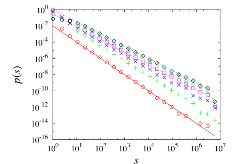
Figure 2: Simulation results of the branching process with the power-law branching ratio with $\gamma=2.01$ ($\circ$), 2.2 ($+$), 2.5 ($\times$), 3.0 ($\Box$), 4.0 ($\triangle$), and 5.0 ($\Diamond$).

The distribution of duration, $i.e.$, the lifetime of a tree growth, can be evaluated similarly alstrom ; harris . Let $r(t)$ be the probability that a branching process stops at or prior to time $t$. Then it is simple to know that $r(t)={\cal Q}(r(t-1))$. For large $t$, $r(t)$ comes close to $1$ and its time variation $r(t)-r(t-1)$ is given by the right hand side of Eq. (6) with $\omega$ replaced by $r(t-1)$ for each region of $\gamma$. Thus the lifetime distribution $\ell(t)=r(t)-r(t-1)$ is given as

$$\ell(t)\sim\left\{\begin{array}[]{ll}t^{-(\gamma-1)/(\gamma-2)}{}{}{}{}{}{}{}&~{}~{}~{}(2<\gamma<3),\\[7.11317pt] t^{-2}(\ln t)^{-1}&~{}~{}~{}(\gamma=3),\\[7.11317pt] t^{-2}&~{}~{}~{}(\gamma>3).\end{array}\right.$$ (8)

Since the distributions of $p(s)$ and $\ell(t)$ are originated from the same tree structures, $p(s){\rm d}s\sim\ell(t){\rm d}t$. Thus from Eqs. (7) and (8), we obtain the dynamic exponent defined via $s\sim t^{z}$ as $z=(\gamma-1)/(\gamma-2)$ for $2<\gamma<3$ and $z=2$ for $\gamma\geq 3$. Following the same steps, we can obtain the exponents $\tau$ and $z$ for more general case where $z_{i}=k_{i}^{\beta}$ with $0\leq\beta\leq 1$. We find $\tau=(\gamma+2\beta-2)/(\gamma+\beta-2)$ and $z=(\gamma+\beta-2)/(\gamma-2)$ for $2<\gamma<\gamma_{c}\equiv\beta+2$, and $\tau=1.5$ and $z=2.0$ for $\gamma>\gamma_{c}$.

Sandpile with uniform threshold— We also consider the case that the threshold height of each node is uniform, while its degree is distributed following the power law. To realize this, we choose the threshold to be $z_{i}=2$ for vertices of degree larger than 1, and $z_{i}=1$ for those of degree 1. Then we modify the dynamic rule accordingly: Toppled grains are transferred to $z_{i}$ randomly selected nearest neighbors, which is similar to that of the Manna model manna . In this case, we obtained $\tau\simeq 1.5$ in all $\gamma>2$ (Fig. 3). This can easily be understood through the branching process analogy: In this case, we have $q_{1}=p_{d}(1)/\langle k\rangle$, $q_{0}=q_{2}=\sum_{k=2}^{\infty}\frac{kp_{d}(k)}{\langle k\rangle}\frac{1}{2}=\frac{1-q_{1}}{2}$, and $q_{k}=0$ for $k>2$. Thus ${\cal Q}(\omega)$ is analytic for all $\omega$, yielding the usual mean-field exponents $\tau=3/2$ and $z=2$ for all $\gamma>2$.

Figure 3: The avalanche size distribution for the static model with uniform threshold. Shown are the case of $\gamma=\infty$ ($\circ$), 3.0 ($\diamond$), and 2.2 ($\Box$). All estimated values of $\tau$ are $1.50\pm 0.05$.

Summary— We have studied the Bak-Tang-Wiesenfeld sandpile model on scale-free networks. To account for the high heterogeneity of the system, the threshold height of each vertex is set to be the degree of the vertex. Numerical simulations suggest that for $2<\gamma<3$ the scaling behavior of the avalanche size distribution differs from the mean-field prediction. By mapping to the multiplicative branching process, we could obtain the asymptotic behaviors of the avalanche size and duration distributions analytically. They are described by novel exponents $\tau$ and $z$ different from the simple mean-field predictions. The result remains the same when threshold contains noise as $z_{i}=\eta_{i}k_{i}$ with $\eta_{i}$ being distributed uniformly in [0,1] and when a new grain is added to a node chosen with probability proportional to the degree of that node. In the case of uniform threshold, on the other hand, we get the mean-field behaviors for all $\gamma>2$.

The fact that $\tau$ increases as $\gamma$ decreases implies the resilience of the network under avalanche phenomena, by the role of the hubs that sustain large amount of grains thus playing the role of a reservoir. This is reminiscent of the extreme resilience of the network under random removal of vertices for $\gamma\leq 3$ bara ; cohen1 ; newman1 . While preparing this manuscript, we have learned of a recent work by Saichev et al. motivated by the study of earthquake avalanches sornette . Their results partly overlap with ours.

- (1) R. Albert and A.-L. Barabási, Rev. Mod. Phys. 74, 47 (2002).
- (2) S.N. Dorogovtsev and J.F.F. Mendes, Adv. Phys. 51, 1079 (2002).
- (3) R. Albert, H. Jeong, and A.-L. Barabási, Nature (London) 406, 378 (2000).
- (4) D.J. Watts, Proc. Natl. Acad. Sci. USA 99, 5766 (2002).
- (5) M.L. Sachtjen, B.A. Carreras, and V.E. Lynch, Phys. Rev. E 61, 4877 (2000).
- (6) A.E. Motter and Y.-C. Lai, Phys. Rev. E 66, 065102 (2002).
- (7) P. Bak, C. Tang, and K. Wiesenfeld, Phys. Rev. Lett. 59, 381 (1987); Phys. Rev. A 38, 364 (1988).
- (8) E. Bonabeau, J. Phys. Soc. Japan 64, 327 (1995).
- (9) P. Alstrøm, Phys. Rev. A 38, 4905 (1988).
- (10) S. Lise and M. Paczuski, Phys. Rev. Lett. 88, 228301 (2002).
- (11) Z. Olami, H.J.S. Feder, and K. Christensen, Phys. Rev. Lett. 68, 1244 (1992); K. Christensen and Z. Olami, Phys. Rev. A 46, 1829 (1992).
- (12) R. Otter, Ann. Math. Stat. 20, 206 (1949).
- (13) K.-I. Goh, B. Kahng, and D. Kim, Phys. Rev. Lett. 87, 278701 (2001).
- (14) A. Aleksiejuk, J.A. Hołyst, and D. Stauffer, Physica A 310, 260 (2002); S.N. Dorogovtsev, A.V. Goltsev, and J.F.F. Mendes, Phys. Rev. E 66, 016104 (2002); M. Leone, A. Vazquez, A. Vespignani, and R. Zecchina, Eur. Phys. J. B 28, 191 (2002); G. Bianconi, Phys. Lett. A 303, 166 (2002).
- (15) R. Cohen, D. ben-Avraham, and S. Havlin, Phys. Rev. E 66, 036113 (2002).
- (16) T.E. Harris, The Theory of Branching Processes (Springer-Verlag, Berlin, 1963).
- (17) J.E. Robinson, Phys. Rev. 83, 678 (1951).
- (18) S.S. Manna, J. Phys. A 24, L363 (1991).
- (19) R. Cohen, K. Erez, D. ben-Avraham, and S. Havlin, Phys. Rev. Lett. 85, 4626 (2000).
- (20) D.S. Callaway, M.E.J. Newman, S.H. Strogatz, and D.J. Watts, Phys. Rev. Lett. 85, 5468 (2000).
- (21) A. Saichev, A. Helmstetter, and D. Sornette, e-print (cond-mat/0305007).