Theory of Kondo lattices and its application to
high-temperature superconductivity and pseudo-gaps in cuprate oxides

Abstract

A theory of Kondo lattices is developed for the $t$-$J$ model on a square lattice. The spin susceptibility is described in a form consistent with a physical picture of Kondo lattices: Local spin fluctuations at different sites interact with each other by a bare intersite exchange interaction, which is mainly composed of two terms such as the superexchange interaction, which arises from the virtual exchange of spin-channel pair excitations of electrons across the Mott-Hubbard gap, and an exchange interaction arising from that of Gutzwiller’s quasi-particles. The bare exchange interaction is enhanced by intersite spin fluctuations developed because of itself. The enhanced exchange interaction is responsible for the development of superconducting fluctuations as well as the Cooper pairing between Gutzwiller’s quasi-particles. On the basis of the microscopic theory, we develop a phenomenological theory of low-temperature superconductivity and pseudo-gaps in the under-doped region as well as high-temperature superconductivity in the optimal-doped region. Anisotropic pseudo-gaps open mainly because of $d\gamma$-wave superconducting low-energy fluctuations: Quasi-particle spectra around $(\pm\pi/a,0)$ and $(0,\pm\pi/a)$, with $a$ the lattice constant, or $X$ points at the chemical potential are swept away by strong inelastic scatterings, and quasi-particles are well defined only around $(\pm\pi/2a,\pm\pi/2a)$ on the Fermi surface or line. As temperatures decrease in the vicinity of superconducting critical temperatures, pseudo-gaps become smaller and the well-defined region is extending toward X points. The condensation of $d\gamma$-wave Cooper pairs eventually occurs at low enough temperatures when the pair breaking by inelastic scatterings becomes small enough.

I Introduction

It is an important issue to elucidate the mechanism of high-temperature (high-$T_{c}$) superconductivity occurring on CuO₂ planes.highTc ; sc1 ; sc2 ; sc3 ; sc4 Cooper pairs can be bound by an exchange interaction.Hirsch According to an early theory,87SC1 ; 87SC2 one of the most possible mechanisms is the condensation of $d\gamma$-wave Cooper pairs bound by the superexchange interaction. Because the on-site Hubbard repulsion is strong in high-$T_{c}$ cuprate oxides, theoretical critical temperatures $T_{c}$ for conventional Bardeen-Cooper-Schrieffer (BCS) superconductivity or the condensation of isotropic $s$-wave Cooper pairs must be very low. As long as the superexchange interaction is antiferromagnetic and it works mainly between nearest neighbors, theoretical $T_{c}$’s for the $d\gamma$ wave are much higher than those for other waves. Many experiments imply that the condensation of $d\gamma$-wave Cooper pairs occurs in the cuprate oxides.Exp-d1 ; Exp-d2

The holehole doping for which observed $T_{c}$’s show a maximum is called an optimal doping; dopings are classified into over- and under-doped ones according to whether they are less or more than the optimal one. Both of normal and superconducting states in the optimal- and over-doped regions can be explained within the theoretical framework of the early theory.87SC2 However, superconductivity in the under-doped region significantly deviates from the prediction of the early theory. Observed $T_{c}$’s decrease with decreasing hole dopings, although theoretical $T_{c}$’s never decrease. Superconducting gaps $\epsilon_{G}(0)$ at $T=0$ K keep increasing with decreasing hole dopings.Shen2 ; Shen3 ; Ding ; Ino ; Renner ; Ido1 ; Ido2 ; Ido4 ; Ekino Experimental ratios of $\epsilon_{G}(0)/k_{B}T_{c}$ are much large than 4.28 given by the early theory.87SC2

Normal states above $T_{c}$ are anomalous in the under-doped region; many experiments imply or show the opening of pseudo-gaps in quasi-particle spectra. For example, the longitudinal nuclear magnetic relaxation (NMR) rate $1/T_{1}T$ becomes smaller as temperatures $T$ are lowered.yasuoka According to angle resolved photoemission spectroscopy (ARPES),Shen2 ; Shen3 ; Ding ; Ino quasi-particle spectra at the chemical potential are swept away around $(\pm\pi/a,0)$ and $(0,\pm\pi/a)$, with $a$ the lattice constant. Scanning tunneling spectroscopy (STS) directly shows the opening of pseudo-gaps.Renner ; Ido1 ; Ido2 ; Ido4 ; Ekino Pseudo-gaps start to open around the so called mean-field critical temperature defined byIdo2 ; Ido4 $T_{c0}\simeq\epsilon_{G}(0)/4k_{B}$, which is much higher than $T_{c}$ in the under-doped region.

The anisotropy of pseudo-gaps deduced from ARPES is similar to that of $d\gamma$-wave superconducting gaps. One may argue that the opening of pseudo-gaps must be a precursor of that of superconducting gaps. On the other hand, the development of pseudo-gaps with decreasing $T$ is not monotonic in several STS data;Ekino ; Ido4 the magnitude of pseudo-gaps shows a maximum at a temperature between $T_{c}$ and $T_{c0}$ and it decreases with decreasing $T$ below the temperature. One may also argue that pseudo-gaps must be suppressed by superconductivity. It is one of the most important issues to clarify how or whether the opening of pseudo-gaps above $T_{c}$ is related with that of superconducting gaps below $T_{c}$.

The cuprate oxides with no hole dopings are Mott-Hubbard’s insulators. Even if holes are doped, they must lie in the strong-coupling regime defined by $U/W\gtrsim 1$, with $U$ the Hubbard repulsion and $W$ the bandwidth. The Hartree-Fock approximation, the random-phase approximation (RPA) and their more or less improved theories such as the self-consistent renormalization (SCR) theory starting from RPA,Moriya the fluctuation exchange (FLEX) approximation starting from RPA and so on are never any relevant approximations for the cuprate oxides; they are relevant only for weakly correlated electron liquids in the weak-coupling regime defined by $U/W\ll 1$.

Hubbard’sHubbard and Gutzwiller’sGutzwiller are within the single-site approximation (SSA) and are relevant for $U/W\gtrsim 1$. When we take both of them,comHubGut we can argue that the density of states must be of a three-peak structure, Gutzwiller’s quasi-particle band at the chemical potential between the lower and upper Hubbard bands. This speculation was confirmed in another SSA theory;OhkawaSlave a narrow band, which is nothing but Gutzwiller’s band, appears at the top of the lower Hubbard band when the electron density is less than half-filling. Gutzwiller’s band is responsible for metallic behavior, and the Mott-Hubbard splitting occurs in both metallic and insulating phases.

The validity of the SSA theories, Hubbard’s and Gutzwiller’s, implies that local fluctuations are responsible for the three-peak structure. Local fluctuations are rigorously considered in one of the best SSA’s that include all the single-site terms.SSAcom Such an SSA is reduced to determining and solving selfconsistently the Anderson model,Mapping which is one of the simplest effective Hamiltonians for the Kondo problem. The Kondo problem has already been solved,singlet ; poorman ; Wilson ; Nozieres ; Yamada ; Yosida ; Exact so that many useful results are available. One of the most essential physics involved in the Kondo problem is that a localized magnetic moment is quenched by local quantum spin fluctuations so that the ground states is a singletsinglet or a normal Fermi liquid.Wilson ; Nozieres The Kondo temperature $T_{K}$ is defined as a temperature or energy scale of local quantum spin fluctuations. The so called Abrikosov-Suhl or Kondo peak in the Kondo problem corresponds to Gutzwiller’s band. Their bandwidth is of the order of $k_{B}T_{K}$, with $k_{B}$ the Boltzmann constant. On the basis of the mapping to the Kondo problem, we argue that lattice systems must show a metal-insulator crossover as a function of $T$: They are nondegenerate Fermi liquids at $T\gg T_{K}$ because local thermal spin fluctuations are dominant, while they are Landau’s normal Fermi liquids at $T\ll T_{K}$ because local quantum spin fluctuations are dominant and magnetic moments are quenched by them. Local-moment magnetism occurs at $T\gg T_{K}$ while itinerant-electron magnetism occurs at $T\ll T_{K}$. Superconductivity can only occur at $T\ll T_{K}$.

The superexchange exchange interaction was originally derived for Mott-Hubbard’s insulators.Kramers ; AndersonSupEch ; Goodenough ; Kondo ; Kanamori One may suspect that it must work only in insulating phases. On the other hand, it was recently shown from a field theoretical approach that it arises from the virtual exchange of spin-channel pair excitation of electrons across the Mott-Hubbard gap.OhkawaExc ; OhkawaFerro Gutzwiller’s band plays no role in this exchange process. It is unquestionable that the superexchange interaction works even in metallic phases as long as the Mott-Hubbard splitting exists. An exchange interaction arising from the virtual exchange of spin-channel pair excitations of Gutzwiller’s quasi-particles also plays a role in metallic phases.OhkawaExc ; OhkawaFerro

A perturbative treatment of exchange interactions including the above two ones starting from an unperturbed state constructed in the SSA is nothing but a theory of Kondo lattices. Because the SSA is rigorous for Landau’s normal Fermi liquids in infinite dimensions,Metzner it can also be formulated as a $1/d$ expansion theory, with $d$ the spatial dimensionality. The theory has already been applied to various phenomena occurring in strongly correlated electron liquids, not only high-$T_{c}$ superconductivityOhkawaSC ; OhkawaSC2 but also itinerant-electron ferromagnetism,OhkawaFerro , the Curie-Weiss law of itinerant-electron magnets,Miyai field-induced ferromagnetism or metamagnetism,Satoh1 itinerant-electron antiferromagnetism,OhkawaAntiferro and so on. The early theory87SC1 ; 87SC2 of high-$T_{c}$ superconductivity is also within a first approximate framework of the theory of Kondo lattices.

Because of anomalous properties of the under-doped region, not a few people speculate that a novel mechanism must be responsible for high-$T_{c}$ superconductivity. On the other hand, we confirmed in solving the Kondo problem that adiabatic or analytical continuity is one of the most important concepts in physics.Yamada ; Yosida ; idea It is, of course, one of the basic assumptions of Landau’s Fermi-liquid theory. The theory of Kondo lattices also relies on this concept. There is no phase transition or no symmetry change between high-$T_{c}$ superconductivity in the optimal-doped region and low-$T_{c}$ superconductivity in the under-doped region. Then, analytical continuity tells us that the theory of Kondo lattices, which can explain superconductivity in the over- and optimal-doped regions, must apply to low-$T_{c}$ superconductivity in the under-doped region. One of the purposes of this paper is to apply the theory of Kondo lattices to low-$T_{c}$ superconductivity and pseudo-gaps in the under-doped region.

This paper is organized as follows: In Sec. II, a theory of Kondo lattices is developed for the $t$-$J$ model. On the basis of the microscopic theory developed in Sec. II, a phenomenological theory of low-$T_{c}$ superconductivity and pseudo-gaps is developed in Sec. III, where several parameters are phenomenologically determined instead of completing self-consistent procedures involved in the microscopic theory. Discussions are given in Sec. IV. Conclusions are given in Sec. V.

II Theory of Kondo lattices

We consider the $t$-$J$ model on a square lattice:

$${\cal H} = -\sum_{ij\sigma}t_{ij}a_{i\sigma}^{\dagger}a_{j\sigma}-\frac{1}{2}J\sum_{\left<ij\right>}({\bf s}_{i}\cdot{\bf s}_{j})$$ (1)

$$+U_{\infty}\sum_{i}a_{i\uparrow}^{\dagger}a_{i\uparrow}a_{i\downarrow}^{\dagger}a_{i\downarrow},$$

with ${\bf s}_{i}=\frac{1}{2}\sum_{\alpha\beta}\left(\sigma_{x}^{\alpha\beta},\sigma_{y}^{\alpha\beta},\sigma_{z}^{\alpha\beta}\right)a_{i\alpha}^{\dagger}a_{i\beta}$, with $\sigma_{x}$, $\sigma_{y}$ and $\sigma_{z}$ the Pauli matrixes, and the summation over $\left<ij\right>$ restricted to nearest neighbors. Here, notations are conventional. The second term is the superexchange interaction. Because we are interested in the cuprate oxides, we assume that $J\!\simeq\!-(0.10$-0.15) eV and the transfer integral between nearest-neighbors is $t_{1}\!\simeq\!(0.4$-0.5) eV:

$$J/|t_{1}|\simeq-(0.2\mbox{--}0.3).$$ (2)

The third term is introduced to exclude any doubly occupied sites, so that $U_{\infty}/|t_{1}|\rightarrow+\infty$. Because no phase transition is possible at nonzero temperatures in two dimensions, we assume that weak three dimensionality exists but the reduction of $T_{c}$ due to it is small.

When Landau’s normal Fermi liquid is considered, the single-particle self-energy is divided into single-site and multi-site terms: $\Sigma_{\sigma}(i\varepsilon_{n},{\bf k})=\tilde{\Sigma}_{\sigma}(i\varepsilon_{n})+\Delta\Sigma_{\sigma}(i\varepsilon_{n},{\bf k})$. The single-site term $\tilde{\Sigma}_{\sigma}(i\varepsilon_{n})$ is identical to the self-energy for a mapped Anderson model, which should be self-consistently determined and solved.Mapping The multi-site term is divided into two terms:

$$\Delta\Sigma_{\sigma}(i\varepsilon_{n},{\bf k})=\Delta\Sigma_{\sigma}({\bf k})+\Delta\Sigma_{\sigma}^{\prime}(i\varepsilon_{n},{\bf k}),$$ (3)

where the first term is independent of energies $i\varepsilon_{n}$ and $\Delta\Sigma_{\sigma}^{\prime}(i\varepsilon_{n},{\bf k})\rightarrow 0$ in the limit of $|\varepsilon_{n}|\rightarrow+\infty$.

First, we construct an unperturbed state in a renormalized SSA, where not only $\tilde{\Sigma}_{\sigma}(i\varepsilon_{n})$ but also $\Delta\Sigma_{\sigma}({\bf k})$ are included. Then, the single-particle Green function is described in such a way that

$$G_{\sigma}^{(0)}(i\varepsilon_{n},{\bf k})=\frac{1}{i\varepsilon_{n}\!\!+\!\mu\!-\!E({\bf k})\!-\!\tilde{\Sigma}_{\sigma}(i\varepsilon_{n})\!-\!\Delta\Sigma_{\sigma}({\bf k})},\!$$ (4)

where $\mu$ is the chemical potential, and $E({\bf k})=-2\sum_{l}t_{l}\eta_{ls}({\bf k})$ is the dispersion relation of electrons, with $t_{l}$ the $l$th nearest-neighbor one of the transfer integral $t_{ij}$ and $\eta_{ls}({\bf k})$ the form factor of the $l$th nearest neighbors:

$$\eta_{1s}({\bf k}) = \cos(k_{x}a)+\cos(k_{y}a),$$ (5a)

$$\eta_{2s}({\bf k}) = \cos[(k_{x}+k_{y})a]+\cos[(k_{x}-k_{y})a],\hskip 22.76228pt$$ (5b)

and so on, with $a$ the lattice constant. The mapping condition to the Anderson model is given byMapping

$$\frac{1}{N}\sum_{\bf k}G_{\sigma}^{(0)}(i\varepsilon_{n},{\bf k})=\tilde{G}_{\sigma}(i\varepsilon_{n}),$$ (6)

with $N$ the number of lattice sites and $\tilde{G}_{\sigma}(i\varepsilon_{n})$ the Green function of the Anderson model; the on-site interaction of the Anderson model should also be infinitely large.

The single-site term is expanded in such a way that

$$\tilde{\Sigma}_{\sigma}(i\varepsilon_{n})=\tilde{\Sigma}_{0}\!\!+\!\bigl{(}1\!-\!\tilde{\phi}_{\gamma}\bigr{)}i\varepsilon_{n}\!\!+\!\bigl{(}1\!-\!\tilde{\phi}_{s}\bigr{)}\!\frac{1}{2}g\mu_{B}H\!+\cdots\!,$$ (7)

in the presence of infinitesimally small fields $H$, with $g$ being the $g$ factor and $\mu_{B}$ the Bohr magneton. The expansion (7) is accurate for $|\varepsilon_{n}|/k_{B}T_{K}\ll 1$; we approximately use it for $|\varepsilon_{n}|/k_{B}T_{K}\lesssim 1$. The Wilson ratio, which appears in the Kondo problem, is defined by

$$\tilde{W}_{s}=\tilde{\phi}_{s}/\tilde{\phi}_{\gamma}.$$ (8)

Because charge fluctuations are suppressed, $\tilde{W}_{s}\rightarrow 2$ in the limit of half-filling or $n\rightarrow 1$,Wilson ; Yamada ; Yosida with $n$ the electron density per site. Theories in SSA give approximate values of $\tilde{\phi}_{\gamma}\simeq 1/|1-n]$.Gutzwiller ; OhkawaSlave The dispersion relation of quasi-particles in the unperturbed state is given by

$$\xi_{0}({\bf k})=\frac{1}{\tilde{\phi}_{\gamma}}\left[E({\bf k})+\tilde{\Sigma}_{0}+\Delta\Sigma_{\sigma}({\bf k})-\mu\right],$$ (9)

and the Green functions are given by $G_{\sigma}^{(0)}(i\varepsilon_{n},{\bf k})=(1/\tilde{\phi}_{\gamma})g_{\sigma}^{(0)}(i\varepsilon_{n},{\bf k})+\mbox{(incoherent part)}$, with

$$g_{\sigma}^{(0)}(i\varepsilon_{n},{\bf k})=\frac{1}{i\varepsilon_{n}-\xi_{0}({\bf k})+i\gamma\ \mbox{sgn}(\varepsilon_{n})},$$ (10)

being the coherent part describing quasi-particles; the incoherent part describes the lower and upper Hubbard bands. Here, a phenomenological life-time width $\gamma$ is introduced; $\mbox{sgn}(x)$ is defined in such a way that $\mbox{sgn}(x)=-1$ for $x<0$ while $\mbox{sgn}(x)=1$ for $x>0$.

When the irreducible polarization function in spin channels is denoted by $\pi_{s}(i\omega_{l},{\bf q})$, the susceptibility of the $t$-$J$ model, which does not include the conventional factor $\frac{1}{4}g^{2}\mu_{B}^{2}$, is given by

$$\chi_{s}(i\omega_{l},{\bf q})=\frac{2\pi_{s}(i\omega_{l},{\bf q})}{1-\left[\frac{1}{2}J({\bf q})+U_{\infty}\right]\pi_{s}(i\omega_{l},{\bf q})},$$ (11)

with

$$J({\bf q})=2J\eta_{1s}({\bf q}).$$ (12)

The irreducible polarization function is also divided into single-site and multi-site terms: $\pi_{s}(i\omega_{l},{\bf q})=\tilde{\pi}_{s}(i\omega_{l})+\Delta\pi_{s}(i\omega_{l},{\bf q})$. The single-site term $\tilde{\pi}_{s}(i\omega_{l})$ is identical to that of the Anderson model, so that the susceptibility of the Anderson model is given by

$$\tilde{\chi}_{s}(i\omega_{l})=\frac{2\tilde{\pi}_{s}(i\omega_{l})}{1-U_{\infty}\tilde{\pi}_{s}(i\omega_{l})}.$$ (13)

An energy scale of local quantum spin fluctuations or the Kondo temperature is defined by

$$k_{B}T_{K}=1/\bigl{[}\tilde{\chi}_{s}(0)\bigr{]}_{T\rightarrow+0}.$$ (14)

Because $U_{\infty}|\tilde{\chi}_{s}(i\omega_{l})|\rightarrow+\infty$ and $U_{\infty}|\chi_{s}(i\omega_{l},{\bf q})|\rightarrow+\infty$, Eq. (11) can also be written in another form:

$$\chi_{s}(i\omega_{l},{\bf q})=\frac{\tilde{\chi}_{s}(i\omega_{l})}{1-\frac{1}{4}I_{s}(i\omega_{l},{\bf q})\tilde{\chi}_{s}(i\omega_{l})},$$ (15)

with

$$I_{s}(i\omega_{l},{\bf q})=J({\bf q})+2U_{\infty}^{2}\Delta\pi_{s}(i\omega_{l},{\bf q}).$$ (16)

This expression is consistent with a physical picture of Kondo lattices: Local spin fluctuations at different sites interact with each other by an intersite exchange interaction. Then, we call $I_{s}(i\omega_{l},{\bf q})$ an exchange interaction.

According to the Ward relation,ward the irreducible single-site three-point vertex function in spin channels is given by $\tilde{\lambda}_{s}(i\varepsilon_{n},i\varepsilon_{n}\!+\!i\omega_{l};i\omega_{l})=\tilde{\phi}_{s}\left[1\!-\!U_{\infty}\tilde{\pi}_{s}(i\omega_{l})\right]$ or

$$\tilde{\lambda}_{s}(i\varepsilon_{n},i\varepsilon_{n}+i\omega_{l};i\omega_{l})=2\tilde{\phi}_{s}/U_{\infty}\tilde{\chi}_{s}(i\omega_{l}),$$ (17)

for $\varepsilon_{n}/k_{B}T_{K}\rightarrow+0$ and $\omega_{l}/k_{B}T_{K}\rightarrow+0$. We approximately use Eq. (17) for nonzero $\varepsilon_{n}$ and $\omega_{l}$. Then, the so called spin-fluctuation mediated interaction in the longitudinal spin channel is given by

$$\left[U_{\infty}\tilde{\lambda}_{s}(0,0;0)\right]^{2}\!\left[\chi_{s}(i\omega_{l},{\bf q})\!-\!\tilde{\chi}_{s}(i\omega_{l})\right]=\tilde{\phi}_{s}^{2}\frac{1}{4}I_{s}^{*}(i\omega_{l},{\bf q}),$$ (18)

with

$$\frac{1}{4}I_{s}^{*}(i\omega_{l},{\bf q}) = \frac{\frac{1}{4}I_{s}(i\omega_{l},{\bf q})}{1-\frac{1}{4}I_{s}(i\omega_{l},{\bf q})\tilde{\chi}_{s}(i\omega_{l})}$$

$$= \frac{1}{4}I_{s}(i\omega_{l},{\bf q})+\left[\frac{1}{4}I_{s}(i\omega_{l},{\bf q})\right]^{2}\!\!\chi_{s}(i\omega_{l},{\bf q}).$$

In Eq. (18), the single-site term is subtracted because it is considered in SSA. The interaction in the transversal channels is also given by Eq. (18); the spin space is isotropic in our system. Because of Eqs. (18) and (19), we call $I_{s}(i\omega_{l},{\bf q})$ a bare exchange interaction, $I_{s}^{*}(i\omega_{l},{\bf q})$ an enhanced one, and $\tilde{\phi}_{s}$ an effective three-point vertex function.

The bare exchange interaction (16) is mainly composed of three terms:

$$I_{s}(i\omega_{l},{\bf q})=J({\bf q})+J_{Q}(i\omega_{l},{\bf q})-4\Lambda(i\omega_{l},{\bf q}).$$ (20)

The first term is the superexchange interaction (12). The second term is an exchange interaction arising from the virtual exchange of pair excitations of quasi-particles. When Eq. (17) is made use of, its lowest-order term in intersite processes is given byOhkawaExc

$$\frac{1}{4}J_{Q}(i\omega_{l},{\bf q})=\frac{\tilde{W}_{s}^{2}}{\tilde{\chi}_{s}^{2}(0)}\bigl{[}P(i\omega_{l},{\bf q})-P_{0}(i\omega_{l})\bigr{]},$$ (21)

with

$$P(i\omega_{l},{\bf q}) = -k_{B}T\sum_{\varepsilon_{n}}\frac{1}{N}\sum_{{\bf k}\sigma}g_{\sigma}^{(0)}(i\varepsilon_{n}+i\omega_{l},{\bf k}+{\bf q})$$ (22)

$$\qquad\times g_{\sigma}^{(0)}(i\varepsilon_{n},{\bf k}).$$

The summation over $\varepsilon_{n}$ can be analytically carried out as is shown in Eq. (78). Here, the single-site term, $P_{0}(i\omega_{l})=(1/N)\sum_{\bf q}P(i\omega_{l},{\bf q})$, is subtracted because it is considered in SSA. The third term corresponds to the so called mode-mode coupling term in the SCR theory.Moriya Because the $\omega$-linear imaginary term in $P_{0}(\omega+i0)$ is cancelled by that in $1/\tilde{\chi}_{s}(\omega+i0)$,OhkawaExc Eq. (15) is approximately given by

$$\chi_{s}(\omega+i0,{\bf q})=\frac{1}{1/\tilde{\chi}_{s}(0)-\frac{1}{4}I_{s}^{\prime}(\omega+i0,{\bf q})},$$ (23)

for $|\omega|\lesssim k_{B}T_{K}$; the exchange interaction is given by

$$I_{s}^{\prime}(\omega\!+\!i0,{\bf q})=J({\bf q})+J_{Q}^{\prime}(\omega\!+\!i0,{\bf q})-4\Lambda(0,{\bf Q}),$$ (24a)

$$\frac{1}{4}J_{Q}^{\prime}(\omega\!+\!i0,{\bf q})=\frac{\tilde{W}_{s}^{2}}{\tilde{\chi}_{s}^{2}(0)}\bigl{[}P(\omega\!+\!i0,{\bf q})-P_{0}(0)\bigr{]},$$ (24b)

with ${\bf Q}=(\pm\pi/a,\pm\pi/a)$.

As is shown in Eq. (3), there are two types of multi-site self-energy corrections. One is the Fock term due to the superexchange interaction. When only the coherent part is considered, it is calculated in such a way that

$$\frac{1}{\tilde{\phi}_{\gamma}}\Delta\Sigma_{\sigma}({\bf k}) = \frac{3}{4}\tilde{W}_{s}^{2}\frac{k_{B}T}{N}\!\sum_{\varepsilon_{n}{\bf q}}J({\bf q})e^{i\varepsilon_{n}0^{+}}\!g_{\sigma}^{(0)}(i\varepsilon_{n},{\bf k}\!+\!{\bf q})$$ (25)

$$= 2J\Xi\eta_{1s}({\bf k}),$$

with

$$\Xi=\frac{3}{4}\tilde{W}_{s}^{2}\frac{k_{B}T}{N}\!\sum_{\varepsilon_{n}{\bf p}}\eta_{1s}({\bf p})e^{i\varepsilon_{n}0^{+}}\!g_{\sigma}^{(0)}(i\varepsilon_{n},{\bf p}).$$ (26)

Here, the factor 3 appears because of three spin channels. According to Gutzwiller’s,Gutzwiller $\tilde{\phi}_{\gamma}\rightarrow+\infty$ in the limit of $n\rightarrow 1$ and the bandwidth of quasi-particles vanishes. When the Fock term is included, however, the bandwidth is about $|J|$ in the unperturbed state even in the limit of $n\rightarrow 1$, if there is no disorder.

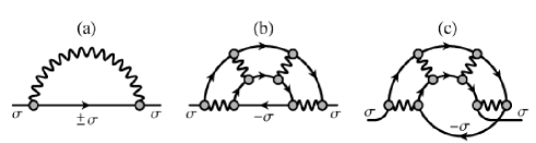
Figure 1: Feynman diagrams for the multi-site self-energy. A solid lines stands for $g_{\sigma}^{(0)}(i\varepsilon_{n},{\bf k})$, a wavy line for $I_{s}^{*}(i\omega_{l},{\bf q})$, and a solid circle for $\tilde{W}_{s}$. Diagram (a) gives the sum of $\Delta\Sigma_{\sigma}({\bf k})$ and $\Delta\Sigma_{\sigma}^{(AF)}(i\varepsilon_{n},{\bf k})$. All the orders of two types of diagrams such as (b) and (c) are considered for $\Delta\Sigma_{\sigma}^{(SC)}(i\varepsilon_{n},{\bf k})$.

So far the unperturbed state is constructed in a renormalized SSA where $\tilde{\Sigma}_{\sigma}(i\varepsilon_{n})$ and $\Delta\Sigma_{\sigma}({\bf k})$ should be self-consistently calculated. Next, $\Delta\Sigma_{\sigma}^{\prime}(i\varepsilon_{n},{\bf k})$ in Eq. (3) is perturbatively considered in terms of $I_{s}(i\omega_{l},{\bf q})$ or $I_{s}^{*}(i\omega_{l},{\bf q})$. We consider two types of corrections shown in Fig. 1: $\Delta\Sigma_{\sigma}^{\prime}(i\varepsilon_{n},{\bf k})=\Delta\Sigma_{\sigma}^{(AF)}(i\varepsilon_{n},{\bf k})+\Delta\Sigma_{\sigma}^{(SC)}(i\varepsilon_{n},{\bf k})$. One arises from antiferromagnetic spin fluctuations:

$$\frac{1}{\tilde{\phi}_{\gamma}}\Delta\Sigma_{\sigma}^{(AF)}(i\varepsilon_{n},{\bf k}) = \frac{k_{B}T}{N}\sum_{\omega_{l}{\bf q}}\tilde{W}_{s}^{2}U_{AF}(i\omega_{l},{\bf q})$$ (27)

$$\times g_{\sigma}^{(0)}(i\varepsilon_{n}\!+\!i\omega_{l},{\bf k}\!+\!{\bf q}),\qquad$$

with

$$U_{AF}(i\omega_{l},{\bf q}) = \frac{3}{4}\Bigl{[}I_{s}^{*}(i\omega_{l},{\bf q})-J({\bf q})\Bigr{]}.$$ (28)

Here, the superexchange interaction $J({\bf q})$, which gives the Fock term, is subtracted.

The other arises from $d\gamma$-wave superconducting fluctuations. We define a reducible polarization function of $d\gamma$-wave particle-particle or Cooper-pair channel by

$$\Pi_{\sigma\sigma^{\prime}}(i\omega_{l},{\bf q}) = \frac{1}{N}\sum_{\bf pk}\eta_{d\gamma}\left({\bf p}\right)\eta_{d\gamma}\left({\bf k}\right)\!\int_{0}^{1/k_{B}T}d\tau e^{i\omega_{l}\tau}$$

$$\times\left<a_{({\bf p}+\frac{1}{2}{\bf q})\sigma}(\tau)a_{(-{\bf p}+\frac{1}{2}{\bf q})-\sigma}(\tau)a_{(-{\bf k}+\frac{1}{2}{\bf q})-\sigma^{\prime}}^{\dagger}a_{({\bf k}+\frac{1}{2}{\bf q})\sigma^{\prime}}^{\dagger}\right>,$$

with

$$\eta_{d\gamma}({\bf k})=\cos(k_{x}a)-\cos(k_{y}a).$$ (30)

Cooper pairs are bound with the enhanced exchange interaction (19). It is expanded in such a way that

$$I_{s}^{*}(i\omega_{l},{\bf q})=I_{0}^{*}(i\omega_{l})+2\sum_{i}I_{i}^{*}(i\omega_{l})\eta_{is}({\bf q}).$$ (31)

Because the nearest-neighbor $I_{1}^{*}(i\omega_{l})$ plays a major role, we only consider it and we ignore other ones. When only ladder diagrams such as those shown in Figs. 1(b) and (c) are considered, fluctuations of different waves are decoupled from each other, so that $\Pi_{\sigma\sigma^{\prime}}(i\omega_{l},{\bf q})$ satisfies the following coupled equation:

$$\Pi_{\sigma\sigma}(i\omega_{l},{\bf q})\!=\!\pi_{d\gamma}(i\omega_{l},{\bf q})\!+\!\frac{1}{2}\pi_{d\gamma}(i\omega_{l},{\bf q})I_{1}^{*}\tilde{\phi}_{s}^{2}\Pi_{\sigma-\sigma}(i\omega_{l},{\bf q})$$

$$\hskip 42.67912pt-\frac{1}{4}\pi_{d\gamma}(i\omega_{l},{\bf q})I_{1}^{*}\tilde{\phi}_{s}^{2}\Pi_{\sigma\sigma}(i\omega_{l},{\bf q}),$$ (32a)

$$\Pi_{\sigma-\sigma}(i\omega_{l},{\bf q})=\frac{1}{2}\pi_{d\gamma}(i\omega_{l},{\bf q})I_{1}^{*}\tilde{\phi}_{s}^{2}\Pi_{\sigma\sigma}(i\omega_{l},{\bf q})$$

$$\hskip 42.67912pt-\frac{1}{4}\pi_{d\gamma}(i\omega_{l},{\bf q})I_{1}^{*}\tilde{\phi}_{s}^{2}\Pi_{\sigma-\sigma}(i\omega_{l},{\bf q}).$$ (32b)

Here, relations of $\Pi_{\sigma-\sigma}(i\omega_{l},{\bf q})=\Pi_{-\sigma\sigma}(i\omega_{l},{\bf q})$ and $\Pi_{\sigma\sigma}(i\omega_{l},{\bf q})=\Pi_{-\sigma-\sigma}(i\omega_{l},{\bf q})$ as well as

$$2\eta_{1}({\bf k}-{\bf p}) = \eta_{1s}({\bf k})\eta_{1s}({\bf p})+\eta_{d\gamma}({\bf k})\eta_{d\gamma}({\bf p})$$ (33)

$$+\eta_{x}({\bf k})\eta_{x}({\bf p})+\eta_{y}({\bf k})\eta_{y}({\bf p}),\hskip 28.45274pt$$

with $\eta_{x}({\bf k})=\sqrt{2}\sin(k_{x}a)$ and $\eta_{y}({\bf k})=\sqrt{2}\sin(k_{y}a)$, are made use of; the energy dependence of $I_{1}^{*}(i\omega_{l})$ is ignored and $I_{1}^{*}=\left<\mbox{Re}[I_{1}^{*}(\omega+i0)]\right>$ is an average over a low-energy region such as $|\omega|\lesssim k_{B}T_{K}$; $\pi_{d\gamma}(i\omega_{l},{\bf q})=\pi_{d\gamma}^{*}(i\omega_{l},{\bf q})/\tilde{\phi}_{\gamma}^{2}$, with

$$\pi_{d\gamma}^{*}(i\omega_{l},{\bf q}) = -\frac{k_{B}T}{N}\sum_{\varepsilon_{n}{\bf k}}\eta_{d\gamma}^{2}\left({\bf k}\right)g_{\sigma}^{(0)}(i\varepsilon_{n},{\bf k}+\mbox{$\frac{1}{2}{\bf q}$})$$ (34)

$$\quad\times g_{\sigma}^{(0)}(-i\varepsilon_{n}-i\omega_{l},-{\bf k}+\mbox{$\frac{1}{2}{\bf q}$}).\qquad$$

The summation over $\varepsilon_{n}$ can be analytically carried out as is shown in Eq. (79). As is discussed in Sec. I, $T_{c}$’s for the $d\gamma$ wave are much higher than $T_{c}$’s for other waves, so that low-energy fluctuations of the $d\gamma$ wave dominate over those of other waves. Then, we consider only them. A superconducting susceptibility for the $d\gamma$ wave is given by

$$\chi_{d\gamma}^{*}(i\omega_{l},{\bf q}) \equiv \tilde{\phi}_{s}^{2}\left[\Pi_{\sigma\sigma}(i\omega_{l},{\bf q})-\Pi_{\sigma-\sigma}(i\omega_{l},{\bf q})\right]$$ (35)

$$= \frac{\displaystyle\tilde{W}_{s}^{2}\pi_{d\gamma}^{*}(i\omega_{l},{\bf q})}{1+\frac{3}{4}I_{1}^{*}\tilde{W}_{s}^{2}\pi_{d\gamma}^{*}(i\omega_{l},{\bf q})}.$$

The self-energy correction is given by

$$\frac{1}{\tilde{\phi}_{\gamma}}\Delta\Sigma_{\sigma}^{(SC)}(i\varepsilon_{n},{\bf k}) = -\frac{k_{B}T}{N}\sum_{\omega_{l}{\bf q}}\tilde{W}_{s}^{2}\eta_{d\gamma}^{2}({\bf k}+\mbox{$\frac{1}{2}$}{\bf q})$$ (36)

$$\times U_{d\gamma}(i\omega_{l},{\bf q})g_{\sigma}^{(0)}(-i\varepsilon_{n}\!-\!i\omega_{l},-{\bf k}\!-\!{\bf q}),\qquad\quad$$

with

$$U_{d\gamma}(i\omega_{l},{\bf q})=\left(\frac{3}{4}I_{1}^{*}\right)^{2}\chi_{d\gamma}^{*}(i\omega_{l},{\bf q}).$$ (37)

In Eqs. (35) and (37), the factor 3 appears together with $I_{1}^{*}$ because of three spin channels.

The Green function renormalized by antiferromagnetic and superconducting fluctuations is given by $G_{\sigma}(i\varepsilon_{n},{\bf k})=g_{\sigma}(i\varepsilon_{n},{\bf k})/\tilde{\phi}_{\gamma}+\mbox{(incoherent part)}$, with

$$g_{\sigma}(i\varepsilon_{n},{\bf k})=\left[\frac{1}{g_{\sigma}^{(0)}(i\varepsilon_{n},{\bf k})}-\frac{1}{\tilde{\phi}_{\gamma}}\Delta\Sigma_{\sigma}^{\prime}(i\varepsilon_{n},{\bf k})\right]^{-1}\!\!,$$ (38)

with $\Delta\Sigma_{\sigma}^{\prime}(i\varepsilon_{n},{\bf k})=\Delta\Sigma_{\sigma}^{(AF)}(i\varepsilon_{n},{\bf k})+\Delta\Sigma_{\sigma}^{(SC)}(i\varepsilon_{n},{\bf k})$. The density of states for quasi-particles is given by

$$\rho^{*}(\varepsilon)=\frac{1}{N}\sum_{\bf k}\rho_{\bf k}^{*}(\varepsilon),$$ (39)

with

$$\rho_{\bf k}^{*}(\varepsilon)=\mbox{Im}\left(-\frac{1}{\pi}\right)g_{\sigma}(\varepsilon+i0,{\bf k}).$$ (40)

III Semi-phenomenological theory

III.1 High-$T_{c}$ superconductivity

On the basis of the formulation in Sec. II, we develop a phenomenological theory. First, we consider the unperturbed state. The dispersion relation $\xi_{0}({\bf k})$ of quasi-particles in the unperturbed state is expanded as

$$\xi_{0}({\bf k})=\mu^{*}-\sum_{i}2t_{i}^{*}\eta_{is}({\bf k}).$$ (41)

Although the expansion coefficients such as $\mu^{*}$, $t_{1}^{*}$, $t_{2}^{*}$, and so on should be self-consistently determined, we treat them as phenomenological parameters. We assume that

$$t_{1}^{*}>0,\quad t_{2}^{*}=-0.3t_{1}^{*},$$ (42)

and we ignore other $t_{l}^{*}$’s. Eq. (42) is consistent with experiment. Furthermore, we treat $t_{1}^{*}$ as an energy unit for the sake of simplicity, although it depends on temperatures, electron densities and so on.

The density of states for quasi-particles in the unperturbed state is given by

$$\rho_{\gamma}(\varepsilon)=\frac{1}{N}\sum_{\bf k}\left(-\frac{1}{\pi}\right)\mbox{Im}g_{\sigma}^{(0)}(\varepsilon+i0,{\bf k}).$$ (43)

According to the Fermi-surface sum rule,FSrule the electron density is given by that of quasi-particles, so that in the limit of $T\rightarrow+0$ and $\gamma\rightarrow+0$

$$n = 2\frac{k_{B}T}{N}\sum_{\varepsilon_{n}{\bf k}}e^{i\varepsilon_{n}0^{+}}g_{\sigma}^{(0)}(i\varepsilon_{n},{\bf k})$$ (44)

$$= 2\!\!\int\!\!d\varepsilon\rho_{\gamma=0}(\varepsilon)f_{\gamma}(\varepsilon)=2\!\!\int\!\!d\varepsilon\rho_{\gamma}(\varepsilon)f_{\gamma=0}(\varepsilon),\quad$$

with

$$f_{\gamma}(\varepsilon)=\frac{1}{2}+\frac{1}{\pi}\mbox{Im}\left[\psi\left(\frac{1}{2}+\frac{\gamma-i\varepsilon}{2\pi k_{B}T}\right)\right].$$ (45)

with $\psi(z)$ the di-gamma function. Note that $\rho_{\gamma=0}(\varepsilon)=(1/N)\sum_{\bf k}\delta[\varepsilon-\xi_{0}({\bf k})]$ and $f_{\gamma=0}(\varepsilon)=1/[e^{\varepsilon/k_{B}T}+1]$.

We assume Eq. (44) even for nonzero $T$ and $\gamma$. Nonzero $\gamma$’s are introduced, partly, for the convenience of numerical processes. Fig. 2(a) shows $\rho_{\gamma}(\varepsilon)$ for several $\gamma$. As long as $\gamma$’s are rather small such as $\gamma/|t_{1}^{*}|\lesssim 0.3$, we expect that essential features are never wiped out by such $\gamma$. Fig. 2(b) shows $n$ as a function of $\mu^{*}$, Fig. 2(c) shows $\mu^{*}$ as a function of $n$, and Fig. 2(d) shows Fermi surfaces for $\gamma=0$ and several $n$.

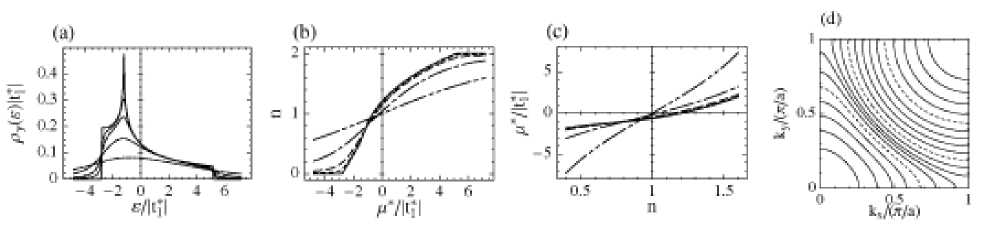
Figure 2: Single-particle properties of the unperturbed state for $T=0$ K, $t_{1}^{*}>0$ and $t_{2}^{*}=-0.3t_{1}^{*}$. (a) Density of states for quasi-particles $\rho_{\gamma}(\varepsilon)$, (b) the electron density $n$ as a function of the effective chemical potential $\mu^{*}$, and (c) $\mu^{*}$ as functions of $n$. In these three figures, solid, dotted, broken, dot-broken and two-dot-broken lines are for $\gamma/|t_{1}^{*}|=10^{-3}$, 0.1, 0.3, 1 and 3, respectively. (d) Fermi surfaces for $\gamma=0$ and 19 electron densities such as $n=0.1\times i$, with $1\leq i\leq 19$ being an integer. Dotted lines show those for $n=$0.5, 1.0 and 1.5. More than half-filling cases $(n>1)$ can be treated, if we take the holehole picture.

     

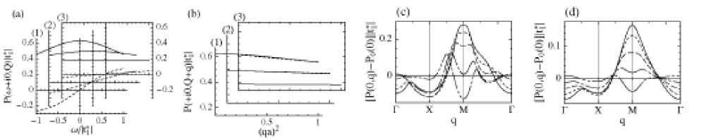
Figure 3: Spin-channel polarization functions: (a) $P(\omega+i0,{\bf Q})|t_{1}^{*}|$ and (b) $P(+i0,{\bf Q}+{\bf q})|t_{1}^{*}|$, with ${\bf Q}=(\pm\pi/2,\pm\pi/2)$, for $n=0.9$ and $k_{B}T/|t_{1}^{*}|=0.1$; $\gamma/|t_{1}^{*}|=0.3$, 1 and 3 are assumed, respectively, in (1), (2) and (3). In Fig. 3(a), solid and dotted lines show the real and imaginary parts, respectively; In Fig. 3(b), solid and dotted lines show those for ${\bf q}\parallel(1,0)$ and ${\bf q}\parallel(1,1)$, respectively; the polarization functions are almost isotropic around Q. (c) $[P(+i0,{\bf q})-P_{0}(+i0)]|t_{1}^{*}|$ for $k_{B}T/|t_{1}^{*}|=\gamma/|t_{1}^{*}|=0.1$, and (d) $[P(+i0,{\bf q})-P_{0}(+i0)]|t_{1}^{*}|$ for $k_{B}T/|t_{1}^{*}|=\gamma/|t_{1}^{*}|=0.3$; solid, dotted, broken, dot-broken and two-dot-broken lines are for $n=1$, 0.9, 0.8, 0.7 and 0.6, respectively. Because $P(+i0,{\bf q})$’s have peaks at wave-numbers different from ${\bf Q}$ for small $n$, effective $\kappa_{s}$’s had better been estimated from Figs. 3(c) and (d) instead of Fig. 3(b).

  

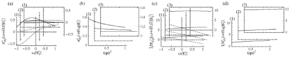
Figure 4: Polarization functions of $d\gamma$-wave Cooper-pair channel: (a) $\pi_{d\gamma}^{*}(\omega+i0,0)|t_{1}^{*}|$, (b) $\pi_{d\gamma}^{*}(+i0,{\bf q})|t_{1}^{*}|$, (c) $1/\pi_{d\gamma}^{*}(\omega+i0,0)|t_{1}^{*}|$ and (d) $1/\pi_{d\gamma}^{*}(+i0,{\bf q})|t_{1}^{*}|$ for $n=0.9$ and $k_{B}T/|t_{1}^{*}|=0.1$. In Figs. 4(a) and (c), solid and dotted lines show real and imaginary parts, respectively. In Figs. 4(b) and (d), solid and dotted lines show those for ${\bf q}\parallel(1,0)$ and ${\bf q}\parallel(1,1)$, respectively; the polarization functions are almost isotropic. In (1), (2) and (3), $\gamma/|t_{1}^{*}|=0.3$, 1 and 3 are assumed, respectively. As $\gamma$’s increase, the $\omega$-linear imaginary term of $1/\pi_{d\gamma}^{*}(\omega+i0,0)$ increases while its $q$-quadratic term decreases.

According to Fermi-liquid relationsYamada ; Yosida and the mapping condition (6), it follows that $\bigl{[}\tilde{\chi}_{s}(0)\bigr{]}_{T\rightarrow+0}=2\tilde{W}_{s}\rho_{\gamma}(0)$ in the limit of $\gamma\rightarrow 0$. In almost half-filling cases $(n\simeq 1)$, $\tilde{W}_{s}\simeq 2$, as is discussed in Sec. II. According to Fig. 2(a), it follows that $\rho_{\gamma}(0)\simeq 0.2/|t_{1}^{*}|$ and $k_{B}T_{K}\simeq 1.2|t_{1}^{*}|$, unless the chemical potential is in the vicinity of the two-dimensional van Hove singularity or $\gamma$’s are extremely large. The specific heat coefficient due to local spin and charge fluctuations is given byYamada ; Yosida $\tilde{\gamma}_{C}=(2/3)k_{B}^{2}\tilde{\phi}_{\gamma}\rho_{\gamma}(0)$.

We take the following phenomenological expressions for susceptibilities:

$$\chi_{s}(\omega+i0,{\bf Q}+{\bf q})=\frac{\chi_{s}(0,{\bf Q})\kappa_{s}^{2}}{\displaystyle\kappa_{s}^{2}+(qa)^{2}-i\omega/\Gamma_{s}},$$ (46a)

$$\chi_{d\gamma}^{*}(\omega+i0,{\bf q})=\frac{\chi_{d\gamma}^{*}(0,0)\kappa_{d\gamma}^{2}}{\displaystyle\kappa_{d\gamma}^{2}+(qa)^{2}+c_{\omega}\omega-i\omega/\Gamma_{d\gamma}},\hskip 28.45274pt$$ (46b)

with ${\bf Q}=(\pm\pi/a,\pm\pi/a)$.

According to an analysis of experimental data,Monthoux $\chi_{s}(0,{\bf Q})=75~{}\mbox{states/eV}$, $1/\kappa_{s}\simeq 2.3$ and $\omega_{SF}=\Gamma_{s}\kappa_{s}^{2}\simeq 14~{}\mbox{meV}$; $\kappa_{s}=0.43$, $\Gamma_{s}=74~{}\mbox{meV}$ and $\chi_{s}(0,{\bf Q})\Gamma_{s}\kappa_{s}^{2}=1.1$. In the optimal-doped region, the specific-heat coefficient is about 14 mJ/mol K², so that $|t_{1}^{*}|\simeq 50~{}\mbox{meV}$. Then, we assume

$$\chi_{s}(0,{\bf Q})\Gamma_{s}\kappa_{s}^{2}\simeq 1,\quad\kappa_{s}\simeq\pi/8,\quad\Gamma_{s}/|t_{1}^{*}|\simeq 1,$$ (47)

for the optimal-doped region.

When the dispersion relation of quasi-particles is given, it is straightforward to calculate polarization functions. For example, Fig. 3 shows $P(\omega+i0,{\bf q})$. Then, we can estimate some of parameters appearing in Eq. (46a). According to Eqs. (23) and (24a), it follows that

$$\frac{1}{\chi_{s}(0,{\bf Q})\Gamma_{s}\kappa_{s}^{2}}=-\frac{\tilde{W}_{s}^{2}}{\tilde{\chi}_{s}^{2}(0)}\mbox{Im}\!\left[\frac{\partial P(\omega\!+\!i0,0)}{\partial\omega}\right]_{\omega=0},$$ (48a)

$$\frac{1}{\chi_{s}(0,{\bf Q})\kappa_{s}^{2}}=-\frac{1}{4}J+\frac{\tilde{W}_{s}^{2}}{\tilde{\chi}_{s}^{2}(0)}\left[\frac{\partial P(0,{\bf Q}\!+\!{\bf q})}{\partial(qa)^{2}}\right]_{{\bf q}=0}.$$ (48b)

Parameters estimated from Fig. 3 together with Eq. (48) for $\gamma/|t_{1}^{*}|=0.3$, $n=0.9$ and $k_{B}T/|t_{1}^{*}|=0.1$ are consistent with those given by Eq. (47).

Fig. 4 shows $\pi_{d\gamma}^{*}(\omega+i0,{\bf q})$. There exists an $\omega$-linear real term in $1/\pi_{d\gamma}^{*}(\omega+i0,{\bf q})$, as is shown in Fig. 4(c). We ignore it and we assume that $c_{\omega}=0$ in Eq. (46b); nonzero $c_{\omega}$ can never play any crucial role in physical properties examined in this paper. According to Eqs. (35) and (46b), it follows that

$$\frac{\tilde{W}_{s}^{2}}{\chi_{d\gamma}^{*}(0,0)\Gamma_{d\gamma}\kappa_{d\gamma}^{2}}=-\mbox{Im}\!\left[\frac{\partial\phantom{\omega}}{\partial\omega}\frac{1}{\pi_{d\gamma}^{*}(\omega\!+\!i0,0)}\right]_{\omega=0},$$ (49a)

$$\frac{\tilde{W}_{s}^{2}}{\chi_{d\gamma}^{*}(0,0)\kappa_{d\gamma}^{2}}=\left[\frac{\partial\phantom{(qa)^{2}}}{\partial(qa)^{2}}\frac{1}{\pi_{d\gamma}^{*}(0,{\bf q})}\right]_{{\bf q}=0}.$$ (49b)

Then, it follows from Figs. 4(c) and (d) that

$$\chi_{d\gamma}^{*}(0,0)\Gamma_{d\gamma}\kappa_{d\gamma}^{2}\simeq\tilde{W}_{s}^{2}/2,\quad\Gamma_{d\gamma}/|t_{1}^{*}|\simeq 1/2,$$ (50a)

for $$\gamma/|t_{1}^{*}|=0.3 n=0.9 k_{B}T/|t_{1}^{*}|=0.1$$, and ;

$$\chi_{d\gamma}^{*}(0,0)\Gamma_{d\gamma}\kappa_{d\gamma}^{2}\simeq\tilde{W}_{s}^{2}/3,\quad\Gamma_{d\gamma}/|t_{1}^{*}|\simeq 1/20,$$ (50b)

for $\gamma/|t_{1}^{*}|=3$, $n=0.9$ and $k_{B}T/|t_{1}^{*}|=0.1$.

Note that there are crucial differences between effects of $\gamma$ on spin and Cooper-pair channel fluctuations: $J$ appears in Eq. (48) but it does not in Eq. (49); the $\omega$-linear imaginary term becomes small with increasing $\gamma$ in the spin channel, as is shown in Fig. 3(a), while it does not in the Cooper-pair channel, as is shown Fig. 4(c). For larger $\gamma$’s, $\Gamma_{s}$’s are larger but $\Gamma_{d\gamma}$’s are smaller. Small $\Gamma_{d\gamma}$’s play a crucial role in the formation of pseudo-gaps studied in Sec. III.2.

When we take Eq. (46), the energy integration in Eqs (27) and (36) can be analytically carried out:

$$\frac{1}{\tilde{\phi}_{\gamma}}\Delta\Sigma_{1}^{(AF)}(\varepsilon+i0,{\bf k}) = g_{AF}\frac{1}{N}\sum_{|{\bf q}|\leq q_{c}}S\Bigl{(}\varepsilon,\xi({\bf k}+{\bf Q}+{\bf q}),\Gamma_{s}\!\left[\kappa_{s}^{2}+(qa)^{2}\right]\Bigr{)},$$ (51a)

$$\frac{1}{\tilde{\phi}_{\gamma}}\Delta\Sigma_{1}^{(SC)}(\varepsilon+i0,{\bf k}) = g_{SC}\frac{1}{N}\sum_{|{\bf q}|\leq q_{c}}\frac{1}{4}\eta_{d\gamma}^{2}({\bf k}+\mbox{$\frac{1}{2}$}{\bf q})S\Bigl{(}\varepsilon,-\xi({\bf k}+{\bf q}),\Gamma_{d\gamma}\!\left[\kappa_{d\gamma}^{2}+(qa)^{2}\right]\Bigr{)}$$ (51b)

$$\simeq g_{SC}\left[\frac{1}{4}\eta_{d\gamma}^{2}({\bf k})\right]\frac{1}{N}\sum_{|{\bf q}|\leq q_{c}}S\Bigl{(}\varepsilon,-\xi({\bf k}+{\bf q}),\Gamma_{d\gamma}\!\left[\kappa_{d\gamma}^{2}+(qa)^{2}\right]\Bigr{)},$$ (51c)

with

$$g_{AF}=3\left[\frac{1}{4}I_{s}(\omega+i0,{\bf Q})\tilde{W}_{s}\right]^{2}\chi_{s}(0,{\bf Q})\Gamma_{s}\kappa_{s}^{2},\qquad g_{SC}=4\left(\frac{3}{4}I_{1}^{*}\tilde{W}_{s}\right)^{2}\chi_{d\gamma}^{*}(0,0)\Gamma_{d\gamma}\kappa_{d\gamma}^{2},$$ (52)

$$S(\varepsilon,x,\Gamma) = -\frac{k_{B}T}{\Gamma}\frac{1}{\varepsilon+i\gamma-x+i\Gamma}+\frac{1}{2\pi}\left[-\psi\!\left(\frac{\Gamma}{2\pi k_{B}T}\right)+\psi\!\left(\frac{-i\varepsilon+ix+\gamma}{2\pi k_{B}T}\right)\right]\frac{1}{\varepsilon+i\gamma-x-i\Gamma}$$ (53)

$$+\frac{1}{2\pi}\left[\psi\!\left(\frac{-i\varepsilon\!+\!\Gamma}{2\pi k_{B}T}\!+\!\frac{1}{2}\right)-\psi\!\left(\frac{\Gamma}{2\pi k_{B}T}\right)-\psi\!\left(\frac{ix\!+\!\gamma}{2\pi k_{B}T}\!+\!\frac{1}{2}\right)+\psi\!\left(\frac{-i\varepsilon\!+\!ix\!+\!\gamma}{2\pi k_{B}T}\right)\right]\frac{1}{\varepsilon\!+\!i\gamma\!-\!x\!+\!i\Gamma}$$

$$+\frac{1}{2\pi}\left[-\psi\!\left(\frac{-i\varepsilon+\Gamma}{2\pi k_{B}T}+\frac{1}{2}\right)+\psi\!\left(\frac{-ix+\gamma}{2\pi k_{B}T}+\frac{1}{2}\right)\right]\frac{1}{\varepsilon-i\gamma-x+i\Gamma}.$$

Because only low-energy antiferromagnetic fluctuations are crucial in Eq. (51a), we use instead of Eq. (28)

$$U_{AF}(\omega\!+\!i0,{\bf q})=\frac{3}{4}\Bigl{[}I_{s}(i\omega_{l},{\bf q})-J({\bf q})\Bigr{]}+\frac{3}{4^{2}}I_{s}^{2}(i\omega_{l},{\bf q})\chi_{s}(i\omega_{l},{\bf q})\simeq 3\left[\frac{1}{4}I_{s}(0,{\bf Q})\right]^{2}\!\chi_{s}(\omega\!+\!i0,{\bf q}).\hskip 28.45274pt$$ (54)

Because we use the phenomenological forms, we restrict the summation over q in Eqs. (51) and we assume that

$$q_{c}a=\pi/3.$$ (55)

Because $q_{c}$ is rather small, we approximately use Eq. (51c) instead of Eq. (51b). In this approximation, there are two interesting properties: When $\kappa_{s}=\kappa_{d\gamma}$ and $\Gamma_{s}=\Gamma_{d\gamma}$, it follows that

$$\frac{1}{g_{AF}}\Delta\Sigma_{\sigma}^{(AF)}(+i0,{\bf k}_{X})=-\frac{1}{g_{SC}}\left[\Delta\Sigma_{\sigma}^{(SC)}(+i0,{\bf k}_{X})\right]^{*}\!,$$ (56a)

for $$X {\bf k}_{X}=(\pm\pi/a,\pm\pi/a) S(0,x,\Gamma)=S^{*}(0,-x,\Gamma) \xi(k_{x}+q_{x},k_{y}+q_{y})=\xi(k_{x}+q_{y}\pm\pi/a,k_{y}+q_{x}\pm\pi/a) {\bf k}={\bf k}_{X}$$ points defined by . In deriving Eq. (56a), two relations of and for are made use of. The other is

$$\Delta\Sigma_{\sigma}^{(SC)}(\varepsilon+i0,{\bf k})=0,$$ (56b)

for ${\bf k}\parallel{\bf k}_{M}$, with ${\bf k}_{M}$ defined by ${\bf k}_{M}=(\pm\pi/a,0)$ and $(0,\pm\pi/a)$. It is certain that the renormalization by $d\gamma$-wave superconducting fluctuations is anisotropic.

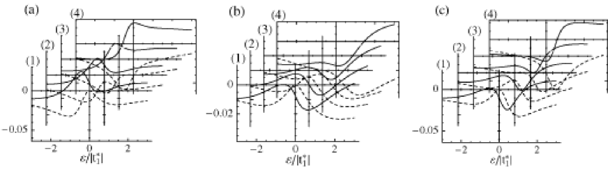
Figure 5: Self-energy corrections: (a) $\Sigma_{\sigma}^{(AF)}(i\varepsilon+i0,{\bf k}_{X})|t_{1}^{*}|/\tilde{\phi}_{\gamma}g_{AF}$ and (b) $\Sigma_{\sigma}^{(AF)}(i\varepsilon+i0,{\bf k}_{M}/2)|t_{1}^{*}|/\tilde{\phi}_{\gamma}g_{AF}$ for $n=0.9$, $\kappa_{s}=\pi/8$ and $\Gamma_{s}/|t_{1}^{*}|=1$; (c) $\Sigma_{\sigma}^{(SC)}(i\varepsilon+i0,{\bf k}_{X})|t_{1}^{*}|/\tilde{\phi}_{\gamma}g_{SC}$ for $n=0.9$, $\kappa_{d\gamma}=\pi/8$ and $\Gamma_{d\gamma}/|t_{1}^{*}|=1$. In (1), (2), (3) and (4), $k_{B}T/|t_{1}^{*}|=0.1$, 0.3, 1 and 3 are assumed, respectively; solid and dotted lines show the real and imaginary parts.

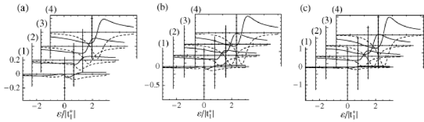
Figure 6: Self-energy corrections: $\Sigma_{\sigma}^{(SC)}(i\varepsilon+i0,{\bf k}_{X})|t_{1}^{*}|/\tilde{\phi}_{\gamma}g_{SC}$ for $n=0.9$, $\kappa_{d\gamma}=\pi/8$ and smaller $\Gamma_{d\gamma}$’s; (a) $\Gamma_{d\gamma}/|t_{1}^{*}|=1/4$, (b) $\Gamma_{d\gamma}/|t_{1}^{*}|=1/8$, and (c) $\Gamma_{d\gamma}/|t_{1}^{*}|=1/16$. In (1), (2), (3) and (4), $k_{B}T/|t_{1}^{*}|=0.1$, 0.3, 1 and 3 are assumed, respectively; solid and dotted lines show the real and imaginary parts.

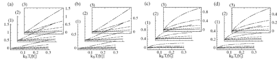
Figure 7: Inelastic life-time widths: Figs. 7(a) and (c) show $\mbox{Im}\bigl{[}\Delta\Sigma_{1}^{(AF)}(+i0,{\bf k}_{X})\bigr{]}|t_{1}^{*}|/\tilde{\phi}_{\gamma}g_{AF}$, which is equal to $-\mbox{Im}\bigl{[}\Delta\Sigma^{(SC)}(+i0,{\bf k}_{X})\bigr{]}^{*}|t_{1}^{*}|/\tilde{\phi}_{\gamma}g_{SC}$ when their corresponding parameters are the same between the two channels; Figs. 7(b) and (d) show $\mbox{Im}\bigl{[}\Delta\Sigma_{1}^{(AF)}(+i0,{\bf k}_{M}/2)\bigr{]}|t_{1}^{*}|/\tilde{\phi}_{\gamma}g_{AF}$. In each figure, $n=0.9$ and $\gamma/|t_{1}^{*}|=0.3$ are assumed; solid, dotted, broken, dot-broken and two-dot-broken lines are for $\Gamma_{s}/|t_{1}^{*}|=1$, 1/2, 1/4, 1/8 and 1/16, respectively. In Figs. 7(a) and (b), $\kappa_{s}$ is assumed to be independent of $T$: (1) $\kappa_{s}=\pi/4$, (2) $\kappa_{s}=\pi/8$, and (3) $\kappa_{s}=\pi/12$. In Figs. 7 (c) and (d), $\kappa_{s}$ is given by Eq. (67); (1) $\kappa_{0}=\pi/4$, (2) $\kappa_{0}=\pi/8$, and (3) $\kappa_{0}=\pi/12$.

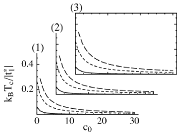
Figure 8: Superconducting $T_{c}$ as a function of the $T$-linear coefficient $c_{0}$: (1) $\gamma=c_{0}k_{B}T$, (2) $\gamma=c_{0}k_{B}T\left[1+\eta_{d\gamma}^{2}({\bf k})/4\right]/2$, and (3) $\gamma=c_{0}k_{B}T\eta_{d\gamma}^{2}({\bf k})/4$. Solid, dotted, and broken lines show $T_{c}$ for $I_{1}^{*}\tilde{W}_{s}^{2}/|t_{1}^{*}|=-1,-2$, and $-3$, respectively.

The electron density is crucial for the nesting of the Fermi surface and the spin susceptibility. Because we use the phenomenological form (46a) for the spin susceptibility, however, the electron density itself is never crucial. Then, we assume $n=0.9$ here and in the following part of this paper. Fig. 5(a) shows $\Delta\Sigma_{\sigma}^{(AF)}(\varepsilon\!+\!i0,{\bf k}_{X})$, Fig. 5(b) shows $\Delta\Sigma_{\sigma}^{(AF)}(\varepsilon\!+\!i0,{\bf k}_{M}/2)$, and Fig. 5(c) and Fig. 6 show $\Delta\Sigma_{\sigma}^{(SC)}(\varepsilon\!+\!i0,{\bf k}_{X})$. Fig. 7 shows the imaginary parts of their static components $(\varepsilon=+i0)$ or inelastic life-time widths of quasi-particles.

Because $|t_{1}^{*}|\simeq 50~{}\mbox{meV}$,

$$|t_{1}/t_{1}^{*}|\simeq 10$$ (57)

in the optimal-doped region. If only the superexchange interaction as large as Eq. (2) is considered, it follows that $|I_{s}(0,{\bf Q}|)/4|t_{1}^{*}|>|J|/|t_{1}^{*}|=(2\mbox{-}3)$ and $|I_{1}^{*}|/|t_{1}^{*}|>|J|/|t_{1}^{*}|=(2\mbox{-}3)$. When we take Eqs. (47) and (50a), $g_{AF}=(12\mbox{-}27)\tilde{W}_{s}^{2}|t_{1}^{*}|^{2}$ and $g_{SC}=(4.5\mbox{-}10)\tilde{W}_{s}^{4}|t_{1}^{*}|^{2}$. If we take $\tilde{W}_{s}\simeq 2$, $g_{AF}\simeq(48\mbox{-}100)|t_{1}^{*}|^{2}$ and $g_{SC}\simeq(72\mbox{-}160)|t_{1}^{*}|^{2}$. On the other hand, observed temperature dependence of resistivity implies

$$(1/\tilde{\phi}_{\gamma})\mbox{Im}\ \Delta\Sigma_{\sigma}(+i0,{\bf k})\simeq-(1\mbox{-}2)k_{B}T,$$ (58)

in the optimal-doped region, so that $g_{AF}$ and $g_{SC}$ should be much smaller than these. For example, if we take

$$\tilde{W}_{s}\simeq(0.7\mbox{-}1),$$ (59)

$g_{AF}\simeq 8(t_{1}^{*})^{2}$ and $g_{SC}\simeq 2(t_{1}^{*})^{2}$. Then, it follows from Figs. 7(a) and (b) that

$$(1/\tilde{\phi}_{\gamma})\mbox{Im}\ \Delta\Sigma_{\sigma}^{(AF)}(+i0,{\bf k})\simeq-k_{B}T,$$ (60a)

for $${\bf k}={\bf k}_{X} {\bf k}={\bf k}_{M}/2$$ and ; it follows from Fig. 7(a) that

$$(1/\tilde{\phi}_{\gamma})\mbox{Im}\ \Delta\Sigma_{\sigma}^{(SC)}(+i0,{\bf k}_{X})\simeq-k_{B}T.$$ (60b)

Eq. (60) is consistent with Eq. (58). As long as $\tilde{W}_{s}\simeq 2$, we cannot explain observed resistivity of the optimal-doping region.

There is a similar drawback for theoretical superconducting critical temperatures $T_{c}$. According to Eq. (35), $T_{c}$’s are given by

$$1+\frac{3}{4}I_{1}^{*}\tilde{W}_{s}^{2}\pi^{*}(0,0)=0.$$ (61)

The imaginary part of the self-energy has a reduction effect of $T_{c}$. Because its static part plays the most crucial role, we consider it as the pair breaking. Because it is almost linear in $T$ as is shown in Fig. 7, we assume a phenomenological form:

$$\gamma=c_{0}\left[c_{1}+(1-c_{1})\frac{1}{4}\eta_{d\gamma}^{2}({\bf k})\right]k_{B}T.$$ (62)

Fig. 8 shows $T_{c}$ for three cases of $c_{1}=0$, $1/2$ and $1$ as a function of $c_{0}$. The reduction of $T_{c}$ is as large as $T_{c0}/T_{c}\simeq 2$ for $c_{0}\simeq(1$-2), with $T_{c0}$ critical temperatures in the absence of any pair breaking. If we take

$$I_{1}^{*}\tilde{W}_{s}^{2}/|t_{1}^{*}|=-(1.5\mbox{-}3),$$ (63)

observed $T_{c}$ in the optimal-doped region can be explained. Eq. (63) is satisfied when we take Eq. (59).

In the formulation in Sec. II, $g_{\sigma}^{(0)}(i\varepsilon_{n},{\bf k})$ appear in Feynman diagrams. These $g_{\sigma}^{(0)}(i\varepsilon_{n},{\bf k})$ had better be renormalized into $g_{\sigma}(i\varepsilon_{n},{\bf k})$ in an improved theory. When this renormalization is made,OhkawaSC2 $\tilde{\phi}_{\gamma}$ is renormalized into $\phi_{\gamma}({\bf k})$ and $\tilde{W}_{s}$ into $W_{s}({\bf k})\equiv\tilde{\phi}_{s}/\phi_{\gamma}({\bf k})$. The energy derivative of the intersite self-energy is estimated from results shown in Figs. 5 and 6, so that $W_{s}({\bf k})$ must be significantly smaller than $\tilde{W}_{s}\simeq 2$.vertex In this paper, however, we simply treat $\tilde{W}_{s}$ as another phenomenological parameter; we assume Eq. (59), that is, $\tilde{W}_{s}\simeq(0.7\mbox{-}1)$.

III.2 Pseudo-gaps and low-$T_{c}$ superconductivity

The following four properties are crucial for the under-doped region. (i) Observed superconducting gaps $\epsilon_{G}(0)$ at $T=0$ K increase with decreasing hole dopings.Shen2 ; Shen3 ; Ding ; Ino ; Renner ; Ido1 ; Ido2 ; Ido4 ; Ekino It implies an increase of the Cooper-pair interaction, that is, the enhanced exchange interaction $I_{1}^{*}$. It is also theoretically argued in Sec. IV that $I_{1}^{*}$ increases with decreasing hole dopings. (ii) As is discussed in Sec. III.1, the energy scale of superconducting fluctuations $\Gamma_{d\gamma}$ is smaller for a larger life-time width $\gamma$ of quasi-particles. (iii) The life-time width $\gamma$ is larger for smaller $\Gamma_{d\gamma}$ or when low-energy superconducting fluctuations are developed, as is shown in Fig. 7. (iv) As hole dopings decrease, cuprate oxides are closer to an antiferromagnetic phase and inelastic scatterings by antiferromagnetic fluctuations more substantially contribute to $\gamma$. Then, we claim that the under-doped region can be characterized by large $\gamma$ and small $\Gamma_{d\gamma}$, or large life-time widths of quasi-particles and low-energy superconducting fluctuations.

An increase of $\gamma$ causes a decrease of $\Gamma_{d\gamma}$ and the decrease of $\Gamma_{d\gamma}$ causes an increase of $\gamma$. Because of this cooperative effect, an increase of $I_{1}^{*}$ and a development of antiferromagnetic fluctuations with decreasing hole dopings causes an increase of $\gamma$ and it eventually causes a large decrease of $\Gamma_{d\gamma}$ and a large increase of $\gamma$. Although this cooperative effect should be examined in a self-consistent way, we treat $\Gamma_{d\gamma}$ as another phenomenological parameter; we assume that it is as small as

$$1/64\lesssim\Gamma_{d\gamma}/|t_{1}^{*}|\lesssim 1/2.$$ (64)

in the under-doped region.

The life-time width $\gamma$ makes the $\omega$ and q dependences of $P(\omega+i0,{\bf q})$ small, as is shown in Figs. 3(a) and (b). Then, the $\omega$ dependence of $1/\chi_{s}(\omega+i0,{\bf q})$ is small in the under-doped region. However, its q dependence can never be as small as that of $1/\chi_{d\gamma}^{*}(\omega+i0,{\bf q})$, because the ${\bf q}$ dependence of the superexchange interaction is never suppressed by $\gamma$. Therefore, $\Gamma_{s}$’s must be large rather than small in the under-doped region. However, we assume for the sake of simplicity that $\Gamma_{s}/|t_{1}^{*}|=1$ even in the under-doped region.

Although $g_{AF}$ and $g_{SC}$ for the under-doped region are larger than those for the optimal-doped one, we assume similar values to those for the optimal-doped one:

$$g_{AF}=8(t_{1}^{*})^{2},\quad g_{SC}=2(t_{1}^{*})^{2}.$$ (65)

     

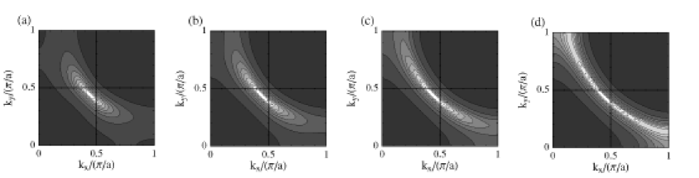
Figure 9: Relative intensities $\rho_{\bf k}(0)$ as functions of $k_{x}$ and $k_{y}$ for $n=0.9$, $k_{B}T/|t_{1}^{*}|=0.1$, $\kappa_{s}=\kappa_{d\gamma}=(\pi/8)$, $\Gamma_{s}/|t_{1}^{*}|=1$, $g_{AF}=8|t_{1}^{*}|^{2}$ and $g_{SC}=2|t_{1}^{*}|^{2}$: (a) $\Gamma_{d\gamma}/|t_{1}^{*}|=1/64$, (b) $\Gamma_{d\gamma}/|t_{1}^{*}|=1/32$, (c) $\Gamma_{d\gamma}/|t_{1}^{*}|=1/16$, and (d) $\Gamma_{d\gamma}/|t_{1}^{*}|=1/2$. When $\Gamma_{d\gamma}$ are small, quasi-particles are well defined only around ${\bf k}=(\pi/2a,\pi/2a)$. Lighter parts have large intensities. The well-defined region extends toward to $(\pi/a,0)$ and $(0,\pi/a)$ as $\Gamma_{d\gamma}$ becomes larger.

     

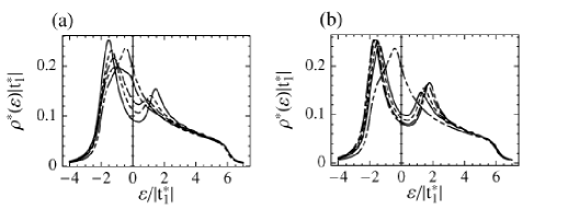
Figure 10: Density of states $\rho^{*}(\varepsilon)$. In Fig. 10(a), parameters are the same as those for Fig. 9: solid, dotted, broken and dot-broken lines correspond to Fig. 9(a), (b), (c) and (d), respectively. In Fig. 10(b), we assume that $\Gamma_{s}/|t_{1}^{*}|=1$, $\Gamma_{d\gamma}/|t_{1}^{*}|=1/64$ and $\kappa_{s}=\kappa_{d\gamma}=(\pi/8)\sqrt{10k_{B}T/|t_{1}^{*}|}$; solid, dotted, broken and dot-broken lines are for $k_{B}T/|t_{1}^{*}|=0.3$, $0.2$, $0.1$ and $0.05$, respectively. In both of Figs. 10(a) and (b), $\rho_{\gamma}(\varepsilon)$ for $\gamma/|t_{1}^{*}|=0.3$ is shown in a two-dot-broken line for comparison. In Fig. 10(a), pseudo-gaps become larger with decreasing $\Gamma_{d\gamma}$. In Fig. 10(b), they become smaller with decreasing $T$.

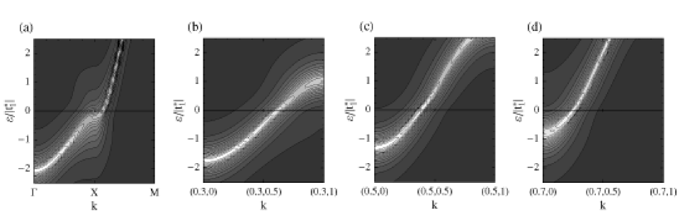
Figure 11: Relative intensities of $\rho_{\bf k}(\varepsilon)$. Parameters are the same as those for Fig. 9(d), and they correspond to those for the optimal-doped region except for the electron density $n=0.9$. Lighter parts have large intensities.

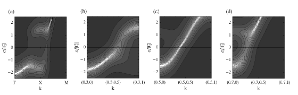
Figure 12: Relative intensities of $\rho_{\bf k}(\varepsilon)$. Parameters are the same as those for Fig. 9(a), and they correspond to those for the under-doped doping region; the electron density is assumed to be $n=0.9$. Lighter parts have large intensities.

Figs. 9(a)-(d) show relative intensities of quasi-particles at the chemical potential, $\rho_{\bf k}^{*}(0)$, in a fourth of the Brillouin zone for four cases such as (a) $\Gamma_{d\gamma}/|t_{1}^{*}|=1/64$, (b) $\Gamma_{d\gamma}/|t_{1}^{*}|=1/32$, (c) $\Gamma_{d\gamma}/|t_{1}^{*}|=1/16$, and (d) $\Gamma_{d\gamma}/|t_{1}^{*}|=1/2$; other parameter are $\gamma=0.3|t_{1}^{*}|$, $k_{B}T/|t_{1}^{*}|=0.1$ and $\kappa_{s}=\kappa_{d\gamma}=\pi/8$. When $\Gamma_{d\gamma}$ are small, spectral intensities are swept away and are almost vanishing around $X$ points, $(\pm\pi/a,0)$ and $(0,\pm\pi/a)$, as is shown in Fig. 9(a). The vanishing of quasi-particle spectra around $X$ points is because of large life-time widths. When $\Gamma_{d\gamma}$ are large, on the other hand, life-time widths are small and the Fermi surface or the Fermi line forms a closed line, as is shown in Fig. 9(d).

Fig. 10(a) shows the density of states for quasi-particles, $\rho^{*}(\varepsilon)$, together with $\rho_{\gamma=0.3|t_{1}^{*}|}(\varepsilon)$ for comparison, as a function of $\varepsilon$ for four values of $\Gamma_{d\gamma}$: $\Gamma_{d\gamma}/|t_{1}^{*}|=1/64$, $1/32$, $1/16$, and $1/2$; other parameter are the same as those for Fig. 9. Pseudo-gap develop as $\Gamma_{d\gamma}$ decrease.

Figs. 11 and 12 show relative intensities of $\rho_{\bf k}^{*}(\varepsilon)$ as a function of $\varepsilon$ and ${\bf k}$. Parameters used for Figs. 11 and 12 are the same as those used for Figs. 9(d) and (a), respectively; Fig. 11 presumably corresponds to the optimal-doped region and Fig. 12 to the under-doped region. A weakly dispersive band around $X$ points in Fig. 11(a) is because of saddle points in the dispersion relation of quasi-particles. The spectra shown in Figs. 11(a)-(d) are rather normal because life-time widths are small. On the other hand, we can see interesting and anomalous properties in Figs. 12(a)-(d) because life-time widths large. Large pseudo-gaps open around $X$ points, and almost dispersionless peaks or flat bands appear along $\Gamma$-$X$ below and above the chemical potential, as is shown in Fig. 12(a). Such flat bands much below the chemical potential must correspond to observed flat bands.Ino Pseudo-gaps become smaller as wavenumbers are closer to ${\bf k}_{M}/2$, as is shown in Figs. 12(b)-(d).

IV Discussions

In an improved theory, the effective transfer integral $t_{1}^{*}$ of quasi-particles is further renormalized by antiferromagnetic and superconducting fluctuations. In this paper, however, we treat $t_{1}^{*}$ for the unperturbed state as one of phenomenological parameters and we take it as the energy unit. Therefore, $T$-dependences discussed in this paper are qualitative.

Low-$T_{c}$ superconductivity in the under-doped region can be explained by large inelastic life-time widths of quasi-particles. For example, $(1/\tilde{\phi}_{\gamma})\mbox{Im}\ \Delta\Sigma_{\sigma}(+i0,{\bf k}_{X})\simeq-(10\mbox{-}20)k_{B}T$ for parameters used to obtain Fig. 12. As is shown in Fig. 8, the reduction of $T_{c}$ is very large for such large life-time widths.

When superconducting gaps as large as $\epsilon_{G}(T)$ open, spin and superconducting low-energy fluctuations with $|\omega|\lesssim\epsilon_{G}(T)$ are depressed and the pair breaking caused by the fluctuations must also be depressed. Therefore, the development of $\epsilon_{G}(T)$ must be very rapid with decreasing $T$. This argument is consistent with experiment.Ekino ; Ido4 It also implies that the reduction of $\epsilon_{G}(0)$ by inelastic scatterings must be very small, so that

$$\frac{\epsilon_{G}(0)}{k_{B}T_{c}}=\frac{\epsilon_{G}(0)}{k_{B}T_{c0}}\frac{T_{c0}}{T_{c}}\simeq 4\frac{T_{c0}}{T_{c}},$$ (66)

with $T_{c0}$ critical temperatures in the absence of any pair breaking. In Sec. III.1, we argue that $T_{c0}/T_{c}\simeq 2$ in the optimal region, so that $\epsilon_{G}(0)/k_{B}T_{c}\simeq 8$. This number 8 is consistent with experiment.Ido4 It is quite reasonable that $\epsilon_{G}(0)/k_{B}T_{c}>8$ or $\epsilon_{G}(0)/k_{B}T_{c}\gg 8$ in the under-doped region.

It is likely that $\kappa_{s}^{2}$ and $\kappa_{d\gamma}^{2}$ decrease almost linearly in $T$ with decreasing $T$ and they vanish at critical temperatures, $T_{N}$ and $T_{c}$, for antiferromagnetism and superconductivity, respectively. Then, we assume that both of $T_{N}$ and $T_{c}$ are zero or very low, so that

$$\kappa_{s}=\kappa_{0}\sqrt{10k_{B}T/|t_{1}^{*}|},\quad\kappa_{d\gamma}=\kappa_{0}\sqrt{10k_{B}T/|t_{1}^{*}|}.$$ (67)

We ignore the $T$-dependence of $\Gamma_{s}$ and $\Gamma_{d\gamma}$. Figs. 7(c) and (d) show inelastic life-time widths of quasi-particles for three cases of $\kappa_{0}=\pi/4$, $\pi/8$ and $\pi/12$. It decreases sublinearly in $T$ rather than linearly. It is likely that resistivity varies in $T^{\alpha}$ with $\alpha<1$ in the under-doped region. It is desirable to develop a microscopic theory in order to predict a precise number of the exponent.

One may argue that the opening of pseudo-gaps is evidence for the formation of preformed Cooper pairs above $T_{c}$. If this scenario is the case, pseudo-gaps must increase with decreasing $T$ at any temperature region. Experimentally, however, pseudo-gaps decrease with decreasing $T$ at a temperature range close to $T_{c}$.Ekino ; Ido4 This observation contradicts the above scenario. Instead, it is a piece of evidence that the opening of pseudo-gaps is because spectral intensities of quasi-particles around $X$ points are swept away by inelastic scatterings. Fig. 10(b) shows $\rho^{*}(\varepsilon)$, together with $\rho_{\gamma=0.3|t_{1}^{*}|}(\varepsilon)$ for comparison, as a function of $\varepsilon$ for four cases such as $k_{B}T/|t_{1}^{*}|=0.3$, $0.2$, $0.1$, and $0.05$; we also assume Eq. (67) with $\kappa_{0}=\pi/8$ as well as $\Gamma_{s}/|t_{1}^{*}|=1$ and $\Gamma_{d\gamma}/|t_{1}^{*}|=1/64$. The decrease of $\kappa_{d\gamma}$ causes an increase of pseudo-gaps, if other parameters are constant. In Fig. 10(b), however, the magnitude of pseudo-gaps decreases with decreasing $T$ because the decrease of life-time widths dominates that of $\kappa_{d\gamma}$. This result is consistent with experiment.Ekino ; Ido4

It is reasonable that $\kappa_{d\gamma}^{2}$ is much smaller below $T_{c0}$ than it is above $T_{c0}\simeq\epsilon_{G}(0)/(4k_{B})$ or that the coefficient of the linear $T$ term in $\kappa_{d\gamma}^{2}$ is quite different between below and above $T_{c0}$. If this is actually the case, pseudo-gaps start to open around $T_{c0}$. It is desirable to study the $T$-dependences of $\Gamma_{d\gamma}$ and $\kappa_{d\gamma}$ in order to predict the $T$-dependence of pseudo-gaps.

When Eq. (46a) is assumed, the longitudinal NMR rate is given by

$$\frac{1}{T_{1}T}\propto\frac{1}{N}\sum_{\bf q}\lim_{\omega\rightarrow+0}\mbox{Im}\frac{\chi_{s}(\omega\!+\!i0,{\bf q})}{\omega}=\frac{\chi_{s}(0,{\bf Q})}{\Gamma_{s}}.$$ (68)

Because life-time widths are large in the under-doped region, $\Gamma_{s}$’s are also large there. When the opening of pseudo-gaps is mainly caused by superconducting fluctuations, $\chi_{s}(0,{\bf Q})$ must be reduced and $\Gamma_{s}$ must be enhanced. It is interesting to examine if the development of superconducting fluctuations can actually explain observed reduction of $1/T_{1}T$.yasuoka It is difficult to explain the reduction of $\chi_{s}(0,{\bf q})$ and $1/T_{1}T$ by the development of antiferromagnetic spin fluctuations.

Experimentally, the so called kink structure is observed in the dispersion relation of quasi-particles determined by ARPES experiment.lanzara Very tiny kink structures can be seen around the chemical potential in Figs. 11(c) and 12(c); they are too tiny to explain ARPES experiment. When pseudo-gaps or superconducting gaps are developed, spectra of antiferromagnetic and superconducting fluctuations may have certain gap-like structures, which are often called resonance modes. It is interesting to examine if such resonance modes actually exist in $\chi_{s}(\omega+i0,{\bf q})$ and $\chi_{d\gamma}^{*}(\omega+i0,{\bf q})$. One may argue that what cause pseudo-gap must cause the kink structure. It is interesting to examine effects of superconducting fluctuations extending in the wavenumber space, whose energies are rather high, as large as $k_{B}T_{K}$ or of the order of the bandwidth of quasi-particles.

 

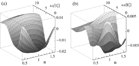
Figure 13: (a) Nearest neighbor $\mbox{Re}\bigl{[}|t_{1}^{*}|P_{1}(\omega+i0)\bigr{]}$ and (b) next-nearest neighbor $\mbox{Re}\bigl{[}|t_{1}^{*}|P_{2}(\omega+i0)\bigr{]}$ as a function of $\omega$ and $n$ for $k_{B}T/|t_{1}^{*}|=0.1$ and $\gamma/|t_{1}^{*}|=1$.

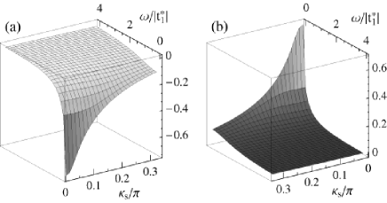
Figure 14: (a) Nearest neighbor $\mbox{Re}\bigl{[}X_{1}(\omega)\bigr{]}$ and (b) next-nearest neighbor $\mbox{Re}\bigl{[}X_{2}(\omega)\bigr{]}$. Note that the directions of $\kappa_{s}$ and $\omega$ axes are opposite to each other between (a) and (b).

Cooper pairs of the $d\gamma$ wave are mainly bound by the enhanced exchange interaction. It is divided into the bare one and the enhanced part, as is shown in Eq. (LABEL:EqIs*2B). As is shown in Eq. (20), the bare one is further divided into three terms. The first term is the superexchange interaction. It is antiferromagnetic, and it is as large as

$$|J/t_{1}^{*}|\simeq(2\mbox{--}3).$$ (69)

The second term is the exchange interaction arising from the virtual exchange of pair excitations of quasi-particles:

$$\frac{1}{4}J_{Q}(\omega+i0,{\bf q})=\frac{2\tilde{W}_{s}^{2}}{\tilde{\chi}_{s}^{2}(0)}\sum_{i=1}^{+\infty}P_{i}(\omega+i0)\eta_{is}({\bf q}),$$ (70)

with

$$P_{i}(\omega+i0)=\frac{1}{N}\sum_{\bf q}P(\omega+i0,{\bf q})\eta_{is}({\bf q}).$$ (71)

Fig. 13(a) shows nearest-neighbor $\mbox{Re}\bigl{[}P_{1}(\omega+i0)\bigr{]}$, and Fig. 13(b) shows next-nearest-neighbor $\mbox{Re}\bigl{[}P_{2}(\omega+i0)\bigr{]}$. The nearest-neighbor one is antiferromagnetic for almost half-filling and is stronger as the electron density is closer to half-filling. However, it is less effective than the superexchange interaction:

$$\frac{2\tilde{W}_{s}^{2}}{\tilde{\chi}_{s}^{2}(0)}\frac{|P_{1}(+i0)|}{|t_{1}^{*}|}\lesssim 0.1.$$ (72)

It is interesting that $\mbox{Re}\bigl{[}P_{1}(\omega+i0)\bigr{]}$ is ferromagnetic for $n<0.7$. The ferromagnetic exchange interaction must play a role in the reduction of $T_{c}$ in the over-doped region. The third term is the so called mode-mode coupling term $-\Lambda(\omega+i0,{\bf q})$. This term works as an repulsive interaction for $d\gamma$-wave Cooper pairs. The enhanced part of Eq. (LABEL:EqIs*2B) is approximately given by

$$\mbox{$\left[\frac{1}{4}I_{s}(0,{\bf Q})\right]^{2}\chi_{s}(\omega+i0,{\bf q})$},$$ (73)

with

$$\chi_{s}(\omega+i0,{\bf q})=\chi_{s}(0,{\bf Q})\kappa_{s}^{2}\sum_{i=0}^{+\infty}X_{i}(\omega+i0)\eta_{is}({\bf q}),$$ (74)

$$X_{i}(\omega+i0)=\frac{1}{N}\sum_{\bf q}\frac{\eta_{is}({\bf q})}{\kappa_{s}^{2}+(qa)^{2}-i\omega/\Gamma_{s}}.$$ (75)

Fig. 14 shows nearest-neighbor $\mbox{Re}\bigl{[}X_{1}(\omega+i0)\bigr{]}$ and next-nearest-neighbor $\mbox{Re}\bigl{[}X_{2}(\omega+i0)\bigr{]}$. The nearest-neighbor one is also antiferromagnetic. As the electron density is closer to half-filling, $\kappa_{s}$’s become smaller so that the enhanced part is stronger. It is also less effective than the superexchange interaction:

$$\left[\frac{1}{4}I_{s}(0,{\bf Q})\right]^{2}\!\frac{\chi_{s}(0,{\bf Q})\kappa_{s}^{2}}{|t_{1}^{*}|}|\mbox{Re}[X_{1}(\omega\!+\!i0)]|\lesssim 0.5,$$ (76)

for $|\omega|\simeq k_{B}T_{K}$. We can argue from Eqs. (69), (72) and (76) that the superexchange interaction is the main part of the pairing interaction in high-$T_{c}$ cuprate oxides, and that the total pairing interaction is larger as the electron density is closer to half-filling.

In the weak-coupling Hubbard model, the spin-fluctuation mediated pairing interaction is given by

$$U^{2}\chi_{s}(\omega+i0,{\bf q}).$$ (77)

Not a few people claim that Cooper pairs must be bound by Eq. (77) in high-$T_{c}$ cuprate oxides. However, this pairing mechanism cannot apply to the cuprate oxides, which certainly lie in the strong-coupling regime. Eq. (77) relevant in the weak-coupling regime is certainly smoothly connected with the pairing mechanism by Eq. (18) or (19) relevant in the strong-coupling regime. However, Eq. (77) is physically different from Eqs. (18) and (73), even if it is similar to them in appearance. Because Eq. (77) arises from the virtual exchange of low-energy pair excitations of quasi-particles, it can also be called an exchange interaction. If we call the superexchange interaction a spin-fluctuation mediated interaction, on the other hand, it sounds impertinent because the energy scale of spin fluctuations responsible for the superexchange interactions is as large as the Hubbard repulsion $U$ and is much larger than the effective Fermi energy of quasi-particles.

V Conclusion

A theory of Kondo lattices is developed for the $t$-$J$ model. On the basis of the microscopic theory, a phenomenological theory of high-$T_{c}$ superconductivity in cuprate oxides is developed; parameters are phenomenologically determined instead of completing the self-consistent procedures involved in the microscopic theory.

In the strong-coupling regime, electrons are mainly renormalized by local quantum spin fluctuations so that the density of states is of a three-peak structure, Gutzwiller’s quasi-particle band at the chemical potential between the lower and upper Hubbard bands. Two bare exchange interactions between quasi-particles are relevant: One is the superexchange interaction, which arises from the virtual exchange of spin-channel pair excitations of electrons between the lower and upper Hubbard bands, and the other is the exchange interaction arising from that of spin-channel pair excitations of quasi-particles themselves. Gutzwiller’s quasi-particles are further renormalized by antiferromagnetic and superconducting fluctuations caused by intersite exchange interactions. The sum of bare exchange interactions including the two are enhanced by low-energy antiferromagnetic fluctuations into the enhanced one. The condensation of $d\gamma$-wave Cooper pairs bound by the enhanced exchange interaction is responsible for high-$T_{c}$ superconductivity in the optimal-doped region.

In the under-doped region, inelastic scatterings by $d\gamma$-wave superconducting low-energy fluctuations cause large life-time widths of quasi-particles around X points; they are almost linear or sublinear in $T$. Anisotropic pseudo-gaps open because spectral intensities of quasi-particles around X points are swept away by strong inelastic scatterings. The development of pseudo-gaps with decreasing $T$ cannot be monotonic; their magnitude must decrease at temperatures close to $T_{c}$. Superconductivity eventually occurs when the pair breaking by inelastic scatterings becomes small enough at low enough $T$’s. Superconducting gaps $\epsilon_{G}(0)$ at $T=0$ K are never much reduced, because low-energy antiferromagnetic and superconducting fluctuations are substantially suppressed by the opening of $\epsilon_{G}(0)$’s themselves and, in particular, because their thermal fluctuations vanish at $T=0$ K.

*

Appendix A

The summations over $\varepsilon_{n}$ in Eqs. (22) and (34) can be analytically carried out. When the analytical continuation such as $i\omega_{l}\rightarrow\omega+i0$ is made, they are given by

$$P(\omega+i0,{\bf q})=\frac{1}{i\pi N}\sum_{{\bf k}}R[\omega,\xi({\bf k}+{\bf q}),\xi({\bf k})],$$ (78)

$$\pi_{d\gamma}^{*}(\omega+i0,{\bf q})=\frac{1}{i2\pi N}\sum_{\bf k}\eta_{d\gamma}^{2}({\bf k})R\left[\omega,\xi\left({\bf k}+\mbox{$\frac{1}{2}$}{\bf q}\right),-\xi\left(-{\bf k}+\mbox{$\frac{1}{2}$}{\bf q}\right)\right],$$ (79)

with

$$R(\omega,\xi_{1},\xi_{2}) = \frac{1}{\omega-\xi_{1}+\xi_{2}}\left[-\psi\left(\frac{1}{2}+\frac{-i\omega+i\xi_{1}+\gamma}{2\pi k_{B}T}\right)+\psi\left(\frac{1}{2}+\frac{i\xi_{2}+\gamma}{2\pi k_{B}T}\right)\right.$$ (80)

$$\left.\hskip 28.45274pt-\psi\left(\frac{1}{2}+\frac{-i\omega-i\xi_{2}+\gamma}{2\pi k_{B}T}\right)+\psi\left(\frac{1}{2}+\frac{-i\xi_{1}+\gamma}{2\pi k_{B}T}\right)\right]$$

$$+\frac{1}{\omega-\xi_{1}+\xi_{2}+i2\gamma}\left[\psi\left(\frac{1}{2}+\frac{-i\omega+i\xi_{1}+\gamma}{2\pi k_{B}T}\right)-\psi\left(\frac{1}{2}+\frac{-i\xi_{2}+\gamma}{2\pi k_{B}T}\right)\right.$$

$$\left.\hskip 28.45274pt+\psi\left(\frac{1}{2}+\frac{-i\omega-i\xi_{2}+\gamma}{2\pi k_{B}T}\right)-\psi\left(\frac{1}{2}+\frac{i\xi_{1}+\gamma}{2\pi k_{B}T}\right)\right],$$

References

- (1) J. G. Bednortz and K. A. Müller, Z. Phys. B64, 189 (1986)
- (2) M. K. Wu, J. R. Ashburn, C. J. Torng, P. H. Hor, R. L. Meng, L. Gao, Z. J. Huang, Y. Q. Wang and C. W. Chu, Phys. Rev. Lett. 58, 908 (1987).
- (3) H. Maeda, Y. Tanaka, M. Fujimoto and T. Asano, Jpn. J. Appl. Phys. 27, L209 (1988).
- (4) Z. Z. Sheng and A. H. Hermann, Nature 332, 138 (1988).
- (5) Y. Tokura, T. Takagi and S. Uchida, Nature 337, 345 (1989).
- (6) J. E. Hirsch, Phys. Rev. Lett. 54, 1317 (1985).
- (7) F. J. Ohkawa, Jpn. J. Appl. Phys. 26, L652 (1987).
- (8) F. J. Ohkawa, J. Phys. Soc. Jpn. 56, 2267 (1987).
- (9) Y. Kitaoka, K. Ishida, G.-q. Zheng, S. Ohsugi and K. Asayama, J. Phys. Chem. Solid. 54, 1385 (1993):
- (10) D. A. Wollman, D. J. Van Harlingen, W. C. Lee, D. M. Ginsberg, and A. J. Leggett, Phys. Rev. Lett. 71, 2134 (1993).
- (11) Holes doped in Mott-Hubbard’s insulators are deficiencies of electrons from the half-filling, while holes doped in normal insulators are those from the complete-filling.
- (12) H. Ding, T. Yokota, J. C. Campuzano, T. Takahashi, M. Randeria, M. R. Norman, T. Mochiku, K. Kadowaki and J. Giapinzakis, Nature 382, 51 (1996).
- (13) J. M. Harris, Z.-X. Shen, P. J. White, D. S. Marshall, M. C. Schabel, J. N. Eckstein and I. Bozovic, Phys. Rev. B 54, R15665 (1996);
- (14) A. G. Loeser, Z.-X. Shen, D. S. Dessau, D. S. Marshall, C. H. Park, P. Fournier and A. Kapitulnik, Science 273, 325 (1996).
- (15) A. Ino, C. Kim, M. Nakamura, T. Yoshida, T. Mizokawa, A. Fujimori, Z.-X. Shen, T. Kakeshita, H. Eisaki and S. Uchida, Phys. Rev. B 65, 094504 (2002)
- (16) Ch. Renner, B. Revaz, J.-Y. Genoud, K. Kadowaki and Ø. Fischer, Phys. Rev. Lett. 80, 149 (1998).
- (17) M. Oda, K. Hoya, R. Kubota, C. Manabe, N. Momono, T. Nakano and M. Ido, Physica C 281, 135 (1997).
- (18) T. Nakano, N. Momono, M. Oda and M. Ido, J. Phys. Soc. Jpn. 67, 2622 (1998).
- (19) R. M. Dipasuphil, M. Oda, N. Momono and M. Ido, J. Phys. Soc. Jpn. 71, 1535 (2002).
- (20) T. Ekino, Y. Sezaki and H. Fujii, Phys. Rev. B 60, 6916 (1999).
- (21) H. Yasuoka, T. Imai and T. Shimizu, Springer Series in Solid State Science 89, String correlation and Superconductivity Springer-Verlag, New York, 1989, p.254.
- (22) T. Moriya, Spin Fluctuations in itinerant Electron Magnetism, Springer Series in Solid-State Science 56, Springer-Verlag, Berlin Heidelberg New York Tokyo, 1985.
- (23) J. Hubbard, Proc. Roy. Soc. A276, 238 (1963); ibid. A281, 401 (1964).
- (24) M. C. Gutzwiller, Phys. Rev. Lett. 10, 159 (1963); Phys. Rev. 134, A293 (1963); ibid. A137, 1726 (1965).
- (25) The configuration of up- and down-spin electrons fluctuates. A characteristic energy scale of the fluctuations is . When high-energy single-particle excitations such as are considered, we can regard the configuration as being almost static. The problem is reduced to one for static disordered systems, which can be treated in the coherent potential approximation (CPA). Hubbard’s is equivalent to CPA and is relevant for . On the other hand, Gutzwiller’s is a variational theory and is relevant for .
- (26) F. J. Ohkawa, J. Phys. Soc. Jpn. 58, 4156 (1989).
- (27) Single-site terms should be renormalized by intersite effects in an eventual theory. Then, various SSA’s are possible depending on the renormalization.
- (28) F. J. Ohkawa, Phys. Rev. B 44, 6812 (1991); J. Phys. Soc. Jpn. 60, 3218 (1991); ibid. 61, 1615 (1991).
- (29) W. Metzner and D. Vollhardt, Phys. Rev. Lett. 62, 324 (1989).
- (30) K. Yosida, Phys. Rev. 147, 223 (1966),
- (31) P. W. Anderson, J. Phys. C 3, 2436 (1970).
- (32) K. G. Wilson, Rev. Mod. Phys. 47, 773 (1975).
- (33) P. Nozières, J. Low. Temp. Phys. 17, 31 (1974).
- (34) K. Yamada, Prog. Theor. Phys. 53, 970 (1975); ibid 54, 316 (1975).
- (35) K. Yosida and K. Yamada, Prog. Theor. Phys. 53, 1286 (1975).
- (36) For reviews on the exact theory by the Bethe method, see for example, N. Andrei, K. Furuya and J. H. Lowenstein, Rev. Mod. Phys. 55, 331 (1983); A. M. Tsvelick and P. B. Wiegmann, Adv. Phys. 32, 453 (1983); A. Okiji and N. Kawakami, Springer Series in Solid State Science (Springer, Berlin, 1988), Vol. 77, p 63; P. Schlottmann, Phys. Rep. 118, 1 (1989).
- (37) H. A. Kramers, Physica 1, 182 (1934).
- (38) P. W. Anderson, Phys. Rev. 79, 350 (1950); ibid. 115, 2 (1959).
- (39) J. B. Goodenough, Phys. Rev. 100, 564 (1955); J. Phys. Chem. Solids 6, 287 (1958).
- (40) J. Kondo, Prog. Theor. Phys. 18, 541 (1957).
- (41) J. Kanamori, J. Phys. Chem. Solids 10, 87 (1959).
- (42) F. J. Ohkawa, J. Phys. Soc. Jpn. 67, 525 (1998).
- (43) F. J. Ohkawa, Phys. Rev. B 65, 174424 (2002).
- (44) F. J. Ohkawa, J. Phys. Soc. Jpn. 61, 631 (1992); J. Phys. Soc. Jpn. 61, 952 (1992); J. Phys. Soc. Jpn. 61, 1157 (1992); Physica B 281-282, 859 (2000); J. Phys. Soc. Jpn. 69, Suppl. A, 13 (2000).
- (45) F. J. Ohkawa, Phys. Rev. B59, 8930 (1999).
- (46) E. Miyai and F. J. Ohkawa, Phys. Rev. B 61, 1357 (2000).
- (47) H. Satoh and F. J. Ohkawa, Phys. Rev. B 57, 5891 (1998); ibid. B 63, 184401 (2001).
- (48) F. J. Ohkawa, J. Phys. Soc. Jpn. 67, 535 (1998); Phys. Rev. B 66, 014408 (2002).
- (49) See for example, P. W. Anderson, Basic Notions of Condensed Matter Physics, Frontier in Physics, Lecture Note Series 55, The Benjamin/Cummings Publishing Company. Inc. 1983.
- (50) J. C. Ward, Phys. Rev. 68, 182 (1950).
- (51) J. M. Luttinger, Phys. Rev. 119, 1153 (1960).
- (52) P. Monthoux and D. Pines, Phys. Rev. B 49, 4261 (1994).
- (53) Multi-site vertex corrections consistent with multi-site self-energy corrections should be considered to satisfy the Ward relation.ward
- (54) A. Lanzara, P. V. Bogdanov, X. J. Zhou, S. A. Keller, D. L. Feng, E. D. Lu, T. Yoshida, H. Eisaki, A. Fujimori, K. Kishio, J.-I. Shimoyama, T. Noda, S. Uchida, Z. Hussain and Z.-X. Shen, Nature 412, 510 (2001).