Correlation Functions of the Magnetization in Thin Films

A. Rebei¹, M. Simionato², G. J. Parker¹

¹Seagate Research Center, Pittsburgh, PA 15222

²Department of Physics and Astronomy, University of Pittsburgh, PA 15260

We calculate the correlation functions of uniform magnetization in thin ferromagnetic films for small deviations from equilibrium, by using a functional formalism. To take account of dissipation and fluctuations consistently, the magnetization is coupled to a bosonic heat bath. The correlation functions show strong dependence on the nature of the coupling between the bath and the system.  Depending on what coupling we choose, we show how the recent results $\left(\text{J. Appl. Phys.}90,5768(2001);\;\text{Phys. Rev. B }65,\right.\\ \left.172417(2002)\right)$ obtained by macroscopic methods can be related to the microscopic treatment adopted here.

1 Introduction

The problem of magnetic noise in nano-systems and in particular in giant-magnetoresistive (GMR) heads is of considerable importance to the physics of magnetic recording. For macroscopic systems, the Landau-Lifshitz-Gilbert equation (LLG) has been used frequently to study thermal fluctuations in magnetic systems mainly through a stochastic approach.brown  Magnetic noise in thin anisotropic films has been recently treated by at least a couple of different methods. smith ; safonov ; jury The first work smith is based on a linearized LLG and application of the fluctuation dissipation theorem (FDT).kubo  The second method safonov is also approximate and based on analogies with the harmonic oscillator.lyberatos  Both calculations are classical, however they give different answers.  Further, in both works it is assumed that the system is close to equilibrium.  To better understand this discrepancy, we study this particular problem of magnetic noise in thin films from a microscopic point of view.  Since we are dealing with a magnetization slightly disturbed from equilibrium, we use bosonic degrees of freedom to describe the magnetization.kittel  Moreover, we use the language of coherent states (CS) to describe the states of the magnetization.glauber  The dissipation is simulated by coupling the magnetization to a bosonic environment. caldeira  The noise spectrum is found by calculating the correlation functions of the magnetization.  We use a functional method borrowed from Field Theory to carry out the general calculation. schwinger ; chou  These methods are attractive because they are equally applicable to highly non-equilibrium situations and very suitable for the many-body problem.  Two of us have already used these methods in a recent paper that addressed the conditions under which a LLG equation can be recovered from a simple quantum model. rebei  The results presented here complement those presented in Ref. rebei .  However this paper can be read independently of our previous work.  The major result of this work is a general expression for the correlation functions from which we can recover both LLG-type correlation functions and oscillator-like correlation functions.  Currently experiments do seem to favor the LLG result however we will not address these questions here. jury ; experiment  We simply show that for systems close to equilibrium, we can have different theories for a large spin.  However, it must be kept in mind that the results obtained are based on a very simple coupling between the magnetization and the bath.  A more realistic coupling such as that of conduction electrons interacting with localized magnetic moments is treated elsewhere.rebei2  In this latter case the use of functional methods is well justified.

The paper is organized as follows. In Sec. II, we first introduce the Hamiltonian for the system considered here.  Then we write this Hamiltonian in an approximate form valid for near-equilibrium cases.  It is shown that in this case the spin Hamiltonian is exactly that of an oscillator.  Since correlation functions of the damped harmonic oscillator in a thermal bath are available in the literature, we deduce from them the corresponding correlation functions for the magnetization.  This result does not apply to LLG-type correlation functions, however, which are deduced from a different coupling between the spin and the bath.  In Sec. III, we review the harmonic oscillator CS and their relation to those of spin CS.  We also write the CS bosonic propagator at finite temperature to be used in subsequent sections and introduce a generating functional for these propagators in real-time.  In Sec. IV, we derive the CS generating functional for the system considered here.  In Sec. V , a normal mode analysis of the noise is carried out.  Here we recover the Safonov-Bertam safonov result in the limit when the range of frequencies are around the resonance (FMR) frequency.  In Sec. VI, we derive the general correlation functions for the magnetization.  The LLG result is shown to follow from the general result by assuming a bath for which the product of the density of states and the coupling constants is linear with frequency.  This is the same condition recovered in Ref. rebei and is independent of the Hamiltonian of the spin system alone. In Sec. VII, we summarize our results.  Finally in an appendix we show how these results can also be obtained form methods of equilibrium statistical mechanics.

2 Quantum Model

In this section, we introduce the quantum model and approximate the magnetization operator by a Bosonic operator stressing the analogies with the harmonic oscillator.  This picture is in general true for close to equilibrium states, irrespective of the equation of motion we are using, i.e., LLG or others.

We consider the following system: A thin magnetic slab with easy axis along the z-axis and a hard axis along the x-axis which are in-plane.  We assume that there is a large external magnetic field $\mathbf{H}$ along the easy axis that keeps the average magnetization in-plane.  We will be interested only in fluctuations around the equilibrium position of the magnetization, i.e., fluctuations in the x and y components of the magnetization.  The Hamiltonian for such a system has the general form $\left(\hbar=1\right)$

$$\widehat{\mathcal{H}} = -H\widehat{S}_{z}-K_{1}\widehat{S}_{z}^{2}+K_{2}\widehat{S}_{x}^{2}+\sum_{k}\omega_{k}b_{k}^{+}b_{k}+V\left(b_{k},b_{k}^{{\dagger}},\widehat{\mathbf{S}}\right),$$ (1)

where  $K_{1}$ and $K_{2}$ are the anisotropy constants.  $\omega_{k}$ is the energy of the $k$-th bath’s oscillator and $\gamma_{k}$’s are the coupling constants, which can be time-dependent. The spin-bath interaction $V$ will be taken linear in $\widehat{\mathbf{S}}$ and the bath variables $b_{k}$. A possible form for $V$ is

$$V\left(b_{k},b_{k}^{{\dagger}},\widehat{\mathbf{S}}\right)=\sum_{k}\left(\gamma_{k}^{\ast}\widehat{S}_{+}b_{k}+\gamma_{k}b_{k}^{+}\widehat{S}_{-}\right).$$ (2)

The Bosonic-type operators for the bath oscillators, $b_{k}$ satisfy the usual commutation relations,

$$\left[b_{k},b_{k}^{+}\right]=\delta_{kk^{\prime}}$$ (3)

For the magnetization, $\widehat{\mathbf{S}}$, we have the following commutation relation

$$\left[\widehat{S}_{+},\widehat{S}_{-}\right]=2\widehat{S}_{z},$$ (4)

where

$$\widehat{S}_{+}=\widehat{S}_{x}+i\widehat{S}_{y},$$ (5)

$$\widehat{S}_{-}=\widehat{S}_{x}-i\widehat{S}_{y}.$$ (6)

$K_{1}$ and $K_{2}$ are the anisotropy constants.  $\omega_{k}$ is the energy of the $k$-th oscillator and $\gamma_{k}$’s are the coupling constants, which can be time-dependent. The Hamiltonian is therefore comprised of three terms: the magnetization (spin term), the spin-reservoir interaction and the reservoir,

$$\widehat{\mathcal{H}}=\widehat{\mathcal{H}}_{S}+\widehat{\mathcal{H}}_{SR}+\widehat{\mathcal{H}}_{R}.$$ (7)

If $S$ is the magnitude of the magnetization, we are interested in the case in which

$$\frac{\left|\widehat{S}-\widehat{S}_{z}\right|}{2S}<<1,$$ (8)

that is deviations from the z-axis are small. For precession around the equilibrium position, i.e., the z-axis, $S_{z}$ can be assumed constant and the Hamiltonian expression for the spin part can be simplified to be of the general form

$$\widehat{\mathcal{H}}_{S}=\frac{1}{2}\left(A\;\widehat{S}_{x}^{2}+B\;\widehat{S}_{y}^{2}\right),$$ (9)

where

$$A=K_{1}+K_{2},\quad B=K_{1}\;.$$ (10)

On average, we have $\langle S_{x}\left(t\right)\rangle=\langle S_{y}\left(t\right)\rangle=0$. To account for thermal fluctuations, we need to calculate the two-point correlation functions of the components of the magnetization, i.e.,

$$\left\langle\widehat{S}_{x}\left(t\right)\widehat{S}_{x}\left(0\right)\right\rangle,\left\langle\widehat{S}_{y}\left(t\right)\widehat{S}_{x}\left(0\right)\right\rangle\quad\ldots$$ (11)

These are the principal quantities that are needed for a full account of the noise or dissipation of the magnetization problem for the model considered here.  Since the Hamiltonian is quadratic, all higher correlation functions are zero.

It is now more appropriate to define the following operators, kittel

$$a=\frac{1}{\left(2S\right)^{\frac{1}{2}}}\widehat{S}_{+}$$ (12)

and

$$a^{+}=\frac{1}{\left(2S\right)^{\frac{1}{2}}}\widehat{S}_{-},$$ (13)

then, we have

$$\widehat{S}_{z}\approx S-a^{+}a$$ (14)

If we normalize by $2S,$ we simply have

$$a=\widehat{S}_{+},$$ (15)

$$a^{+}=\widehat{S}_{-}$$ (16)

and

$$\widehat{S}_{x}=\frac{1}{2}\left(a+a^{+}\right),$$ (17)

$$\widehat{S}_{y}=\frac{1}{2i}\left(a-a^{+}\right).$$ (18)

Therefore

$$\left|\frac{1}{2}-S_{z}\right|<<1\;.$$ (19)

The operators $a$ and $a^{+}$ then behave as bosonic degrees of freedom, i.e., the magnetization behaves, in this approximation, like a harmonic oscillator, vanvleck

$$\left[a,a^{+}\right]=\frac{\widehat{S}_{z}}{S}\approx 1.$$ (20)

If we rewrite the Hamiltonian in terms of these operators, we find

$$\widehat{\mathcal{H}} = \Omega a^{+}a+V\left(a,a^{+}\right)$$

$$+\sum_{k}\omega_{k}b_{k}^{+}b_{k}-\sum_{k}\gamma_{k}\left(a^{+}b_{k}+b_{k}^{+}a\right),$$

where

$$\Omega=H+K_{1}+\frac{1}{2}K_{2},$$ (22)

and the potential $V$ is in this case equal to

$$V\left(a^{+},a\right)=\frac{1}{4}K_{2}\left(aa+a^{+}a^{+}\right).$$ (23)

In general, the spin part has the form

$$\widehat{\mathcal{H}}_{S}=\Omega a^{+}a+V\left(a^{+},a\right).$$ (24)

The calculation presented below can be tailored to deal with any polynomial $V$ which will give rise to some type of Feynman rules.orland

Before we end this section, we would like to point out the analogy between the spin problem and the harmonic oscillator problem when they are coupled to a bosonic bath.  For a quantum oscillator, the Hamiltonian is

$$\widehat{\mathcal{H}}_{0}=\frac{\widehat{p}^{2}}{2M}+V\left(\widehat{q}\right)=\frac{\widehat{p}^{2}}{2M}+\frac{1}{2}M\omega_{0}^{2}\widehat{q}^{2},$$ (25)

while for the spin Hamiltonian, we have

$$\widehat{\mathcal{H}}_{S} = \frac{A}{2}\widehat{S}_{x}^{2}+\frac{B}{2}\widehat{S}_{y}^{2}$$ (26)

$$= \frac{\widehat{S}_{y}^{2}}{2M}+\frac{1}{2}M\omega_{0}^{2}\widehat{S}_{x}^{2}$$ (27)

which means

$$A=M\omega_{0}^{2},\qquad B=\frac{1}{M}.$$ (28)

The commutation relation for the harmonic oscillator

$$\left[\widehat{q},\widehat{p}\right]=i,$$ (29)

and for a spin, we similarly have

$$\left[\widehat{S}_{x},\widehat{S}_{y}\right]=i\widehat{S}_{z}.$$ (30)

If $\widehat{S}_{z}$ is a constant of motion, we can replace the operator $\widehat{S}_{z}$ by its average value and normalize the remaining components by it.  Both systems, the harmonic oscillator and the spin, are equivalent if they are coupled the same way to the bath.  Most works on the harmonic oscillator case involved linear coupling to the bath. Reference grabert gives an exhaustive treatment of this problem.  If for each $b_{k},b_{k}^{{\dagger}}$, we define two new real operators $x_{k}$ and $p_{k}$, such that

$$b_{k}=\frac{1}{\sqrt{2}}\left(\sqrt{\omega_{k}}x_{k}+i\frac{p_{k}}{\sqrt{\omega_{k}}}\right)$$ (31)

and

$$b_{k}^{+}=\frac{1}{\sqrt{2}}\left(\sqrt{\omega_{k}}x_{k}-i\frac{p_{k}}{\sqrt{\omega_{k}}}\right).$$ (32)

Then the coupling is given by

$$\widehat{\mathcal{H}}=-q\sum_{k=1}^{N}\gamma_{k}x_{k}$$ (33)

The equations of motion are given by the Heisenberg equation.  For the harmonic oscillator, we have

$$i\overset{\cdot}{\widehat{q}}=\left[\widehat{q},\widehat{H}\right],\;\;\;\;\;i\overset{\cdot}{\widehat{p}}=\left[\widehat{p},\widehat{H}\right],$$ (34)

with similar equations for the magnetization with $q\rightarrow\widehat{S}_{x}$ and $p\rightarrow\widehat{S}_{y}$. For the linear coupling, Eq.$\left(\ref{coupling}\right)$, the correlation function of the position,

$$C_{qq}\left(t\right)=\frac{1}{2}\langle q\left(t\right)q+qq\left(t\right)\rangle,$$ (35)

is equal to grabert

$$C_{qq}\left(t\right)=\frac{1}{M}\int\frac{d\omega}{2\pi}\frac{\omega\alpha\left(-i\omega\right)}{\left(\omega_{0}^{2}-\omega^{2}\right)^{2}+\omega^{2}\alpha\left(-i\omega\right)^{2}}\;\coth\frac{\beta\omega}{2}\cos\left(\omega t\right),$$ (36)

where

$$\alpha\left(z\right)=\frac{1}{M}\sum_{k=1}^{N}\frac{\gamma_{k}^{2}}{2\omega_{k}}\;\frac{2z}{\omega_{k}^{2}+z^{2}},$$ (37)

and $\beta$ is inverse temperature $1/kT$ with $k$ the Boltzmann constant.  For Ohmic dissipation, the damping kernel is without memory and hence $\alpha\left(z\right)$ is a constant.  This is achieved by having a bath with spectral density linear in frequency.  In this case the magnetization correlation function for the $x-$component in the high temperature limit is

$$C_{xx}\left(\omega\right)=2\alpha kT\;\frac{B}{\left(\omega_{0}^{2}-\omega^{2}\right)^{2}+\left(\alpha\omega\right)^{2}}.$$ (38)

From Eq. $\left(\ref{analogy}\right)$, the (FMR) frequency $\omega_{0}$ is, as expected, equal to $\sqrt{AB}$.  This result may not however be observed for a spin variable, since the interaction term has the unusual form of having only one component coupled to the bath,

$$\widehat{\mathcal{H}}_{SR}=-\sum_{k=1}^{N}\frac{\gamma_{k}}{2\sqrt{2\omega_{k}}}\left(b_{k}+b_{k}^{+}\right)\widehat{S}_{x}.$$ (39)

Here it is the $x-$component of the magnetization which is coupled to the bath.  Hence the coupling in Eq. $\left(\ref{Ham}\right)$ seems more reasonable for a spin variable, in general.  The question of counter-terms will not be treated here and any shift in the frequency will be absorbed.  Reference ford gives a detailed treatment of these terms within the models treated here.

3 The Coherent State Representation : Equilibrium and Non-Equilibrium Dynamics

Here we first review the Bosonic coherent state representation and then show how it can be used within the path-integral formulation of quantum mechanics.  Some typical formulas are presented here for transition rates between two states.  All the results are based on the standard Gaussian formula for path integrals.

3.1 Coherent States

Coherent states are the natural representation for semi-classical calculations.  A Gaussian wave-packet for a harmonic oscillator with minimum uncertainty is a coherent state.   They are formally defined as eigenstates of the annihilation operator glauber

$$a\left|\alpha\right\rangle=\alpha\left|\alpha\right\rangle$$ (40)

where $\alpha$ is a complex number.  Usually the ground state is defined as the state with zero quanta,

$$a\left|0\right\rangle=0.$$ (41)

For spin coherent states, the ground state is taken to be the state with the highest weight $J$, or zero deviation from highest weight

$$\left|0\right\rangle_{S}=\left|J,J\right\rangle,\qquad S^{2}=J\left(J+1\right).$$ (42)

For Bosons, the Hilbert space ( or space of all possible states) is a linear combination of all state vectors, $\left\{\left|n\right\rangle\right\}$, such that

$$\left|n\right\rangle=\frac{1}{\sqrt{n!}}\left(a^{+}\right)^{n}\left|0\right\rangle.$$ (43)

These states form an orthonormal basis.  Coherent states may then be written in terms of these states.  We have

$$\left|\alpha\right\rangle=e^{\alpha a^{+}}\left|0\right\rangle.$$ (44)

Spin coherent states are defined in a similar way.  We have

$$\left|\alpha\right\rangle=\frac{1}{1+\left|\alpha^{2}\right|}e^{\alpha a^{+}}\left|0\right\rangle_{S},$$ (45)

where the extra factor in front is due to the constraint that $S^{2}$ is constant. An important operator relation for a path-integral representation is the decomposition of the unit operator in terms of coherent projection operators

$$\int\frac{d\alpha^{\ast}d\alpha}{2\pi i}e^{-\alpha^{\ast}\alpha}\left|\alpha\right\rangle\left\langle\alpha\right|=\widehat{1},$$ (46)

which is used in the discretization of the path integral. orland The coherent states form an over-complete basis.

In all the calculations carried out below, we keep repeatedly using the fundamental result for the Gaussian integral,

$$\int\underset{i}{\Pi}d\mu\left(\phi_{i}\right)\exp\left\{-\sum_{ij}\phi_{i}^{\ast}A_{ij}\phi_{j}+\sum_{i}\alpha_{i}^{\ast}\phi_{i}\right.\left.+\sum_{i}\phi_{i}^{\ast}\alpha_{i}\right\}$$ (47)

$$\;\;\;\;\;\;\;\;\;=\frac{1}{\det A}\,\,\,\exp\left\{-\sum_{ij}\alpha_{i}^{\ast}\left(A^{-1}\right)_{ij}\alpha_{j}\right\}.$$

3.2 Propagators

A typical propagator that shows up often in the calculations of the correlation functions is associated with a Hamiltonian that has the following general form,

$$\widehat{\mathcal{H}}\left[{J},{J}^{\ast}\right]=\Omega a^{+}a-J(t)a^{+}-J^{\ast}(t)a$$ (48)

where $J(t)$ is a time-dependent external source.  The kernel of the evolution operator from an initial state $z_{i}$ to a final state $z_{f}$ is given by orland

$$\mathcal{K}_{J}\left(\overline{z}_{f},t_{f},z_{i},t_{i}\right)=\left\langle z_{f},t_{f}\quad|\quad z_{i},t_{i}\right\rangle=e^{iS\left[{J},{J}^{\ast}\right]}.$$ (49)

Applying the Gaussian formula, Eq.$\left(\ref{gaussian}\right)$, with the boundary conditions

$$z\left(t_{i}\right) = z_{i},$$ (50)

$$\overline{z}\left(t_{f}\right) = \overline{z}_{f},$$ (51)

gives the phase $S$,

$$S\left[{J},{J}^{\ast}\right] = -i\overline{z}_{f}e^{-i\Omega\left(t_{f}-t_{i}\right)}+\int_{t_{i}}^{t_{f}}dt\left[\overline{z}_{f}e^{-i\Omega\left(t_{f}-t\right)}J(t)+J^{\ast}(t)e^{-i\Omega\left(t-t_{i}\right)}z_{i}\right]$$

$$+i\int_{t_{i}}^{t_{f}}dt\;\int_{t_{i}}^{t_{f}}dt^{\prime}\;J^{\ast}\left(t\right)e^{-i\Omega\left(t-t^{\prime}\right)}J\left(t^{\prime}\right)\Theta\left(t-t^{\prime}\right).$$

$\Theta\left(t\right)$ is the unit step function.  In using coherent states, the variables $z$ and $\overline{z}$ are not necessarily related by complex conjugation.  They have to be treated as independent.

3.3 Partition Function: Euclidean formulation

This formulation is useful to calculate thermodynamic equilibrium properties of a system.  In this case, the partition function is obtained through a calculation of diagonal propagators in imaginary time,

$$\tau=it,\qquad 0\leq\tau\leq\beta$$ (53)

In the coherent state representation, the partition function is written

$$\mathbb{Z}_{\beta}\left[J,J^{\ast}\right]=\int d\mu(z)e^{-z^{\ast}z}\left\langle z\left|\mathbf{T}\exp\left\{-\int_{0}^{\beta}d\tau\widehat{\mathcal{H}}\left[J,J^{\ast}\right]\right\}\right|z\right\rangle,$$ (54)

where $\mathbf{T}$ is the imaginary time ordering operator. The integrals in this partition function are all Gaussian and hence can be easily calculated with the aid of Eq.$\left(\ref{gaussian}\right)$.  We get

$$\mathbb{Z}_{\beta}\left[J,J^{\ast}\right]=n\left(\omega\right)\exp\left\{{\beta\omega}+S\left[J,J^{\ast}\right]\right\}$$ (55)

where

$$S\left[J,J^{\ast}\right]=\int_{0}^{\beta}d\tau\int_{0}^{\beta}d\tau^{\prime}J^{\ast}(\tau)D\left(\tau,\tau^{\prime}\right)J(\tau^{\prime}),$$ (56)

$D\left(\tau,\tau^{\prime}\right)$ is the Feynman propagator of this model

$$D\left(\tau,\tau^{\prime}\right)=\langle\mathbf{T}\left(a^{+}\left(\tau\right)a\left(\tau^{\prime}\right)\right)\rangle.$$ (57)

It is not difficult to find that it is given by

$$D\left(\tau,\tau^{\prime}\right)=n\left(\omega\right)e^{-\omega\left(\tau-\tau^{\prime}-\frac{\beta}{2}\right)}\left[e^{\beta\frac{\omega}{2}}\theta\left(\tau-\tau^{\prime}\right)+e^{-\beta\frac{\omega}{2}}\theta\left(\tau^{\prime}-\tau\right)\right],$$ (58)

where

$$n\left(\omega\right)=\frac{1}{e^{\beta\omega}-1}$$ (59)

is the Bose-Einstein distribution.  Its Fourier transform coincides with the well known Matsubara propagator

$$D(\omega_{n},\omega)=\frac{1}{i\omega_{n}+\omega},\quad\omega_{n}=2\pi\,n\,T,\quad n=0,\pm 1,\pm 2,...\;.$$

This last propagator is essential for any calculations that involve calculating expectation values of any observable.rivers  In the appendix we show how to use this method to calculate correlation functions.

3.4 Real-Time Formulation: Dynamics

The real-time formulation deals with non-equilibrium questions.  In this case we can derive equations of motion for any observables. chou  This is the method we adopt in the calculations of the correlation functions of the magnetization. For a general operator $\mathcal{O},$ its average value at any time $t$ is given in terms of the density matrix $\rho$,

$$\left\langle\mathcal{O}\left(t\right)\right\rangle=Tr\left\langle\rho\mathcal{O}\left(t\right)\right\rangle.$$ (60)

The operator $\mathcal{O}$ is in the Heisenberg picture,

$$\mathcal{O}(t)=e^{i\widehat{\mathcal{H}}t}\mathcal{O}e^{-i\widehat{\mathcal{H}}t}.$$ (61)

Therefore the average of the observable $\mathcal{O}$ at time $t$ can be written in terms of that at $t=0$,

$$\left\langle\mathcal{O}(t)\right\rangle=Tr\left(\rho e^{i\widehat{\mathcal{H}}t}\mathcal{O}e^{-i\widehat{\mathcal{H}}t}\right).$$ (62)

This latter average can be written in terms of path integrals as in the equilibrium case.  First we define the operators $\mathcal{K}$ and $\overline{\mathcal{K}}$.  The operator $\mathcal{K}$ is a forward propagator and is defined as follows,

$$\mathcal{K}\left[J_{1},J_{1}^{\ast}\right] = \mathbf{T}\exp\left\{{-i}\int_{t_{i}}^{t_{f}}\left(\widehat{\mathcal{H}}-J_{1}^{\ast}a-J_{1}a^{+}\right)dt\right\}$$

$$= \mathbf{T}\exp\left\{{-i}\int\left(\widehat{\mathcal{H}}-F_{1}^{x}S_{x}-F_{1}^{y}S_{y}\right)dt\right\}$$

$\mathbf{T}$ is a time ordering operator.  $\overline{\mathcal{K}}$ is a backward operator and is therefore defined in terms of anti-ordered time operator $\overline{\mathbf{T}}$,

$$\overline{\mathcal{K}}\left[J_{2},J_{2}^{\ast}\right] = \overline{\mathbf{T}}\exp\left\{{-i}\int_{t_{f}}^{t_{i}}\left(\widehat{\mathcal{H}}-J_{2}^{\ast}a-J_{2}a^{+}\right)dt\right\}$$

$$= \overline{\mathbf{T}}\exp\left\{{-i}\int\left(\widehat{\mathcal{H}}-F_{2}^{x}S_{x}-F_{2}^{y}S_{y}\right)dt\right\},$$

where $\mathbf{F}_{1}$ and $\mathbf{F}_{2}$ are real external fields which are coupled to the transverse components of the magnetization.  Similar to the equilibrium case, we define a generating functional

$$\mathbb{Z}\left[\mathbf{J},\mathbf{J}^{\ast}\right]=Tr\left\{\rho\left[J_{3},J_{3}^{\ast}\right]\overline{\mathcal{K}}\left[J_{2},J_{2}^{\ast}\right]\mathcal{K}\left[J_{1},J_{1}^{\ast}\right]\right\}.$$ (65)

$\mathbf{J}$ is now the three-vector $\left(J_{1},J_{2},J_{3}\right)$.  The density matrix $\rho$ is assumed of the form

$$\rho\left[J_{3},J_{3}^{\ast}\right] = {\mathbf{T}}_{I}\exp\left\{-\int_{0}^{\beta}\left(\widehat{\mathcal{H}}-J_{3}^{\ast}a-J_{3}a^{+}\right)d\tau\right\}$$

$$= {\mathbf{T}}_{I}\exp\left\{-\int_{0}^{\beta}\left(\widehat{\mathcal{H}}-F_{3}^{x}S_{x}-F_{3}^{y}S_{y}\right)d\tau\right\},$$

where $\mathbf{T}_{I}$ is now a time-ordering operator along the imaginary time axis.  Hence, all correlation functions can be obtained from the coefficients of the Taylor expansion of the functional $\mathbb{Z}\left[\mathbf{J},\mathbf{J}^{\ast}\right]$ around $\mathbf{J}=\mathbf{J}^{\ast}=0$ (or $\mathbf{F}_{1}=\mathbf{F}_{2}=\mathbf{F}_{3}=0$).  For example, the average value of the $x-$component of the magnetization at time $t$ can be found by differentiating $\mathbb{Z}$ with respect to $F_{1}^{x}$ at the same time $t$,

$$\frac{1}{\mathbb{Z}}\left.\frac{\delta\mathbb{Z}\left[\mathbf{J},\mathbf{J}^{\ast}\right]}{\delta F_{1}^{x}\left(t\right)}\right|_{F=0}=-\left\langle S_{x}\left(t\right)\right\rangle.$$ (67)

Next we define another functional $\mathbb{W}$ which at equilibrium becomes the thermodynamic potential of the system,

$$\mathbb{Z}\left[\mathbf{F}_{i=1,2,3}\right]=\exp\left\{i\mathbb{W}\left[F\right]\right\}.$$ (68)

The functional $\mathbb{W}$, as will be seen below, is the more appropriate functional to calculate and expand in powers of $\mathbf{J}$ and $\mathbf{J}^{\ast}$ (or $\mathbf{F}$).  Therefore, we have for averages and two-point correlation functions,

$$\left.\frac{\delta\mathbb{W}}{\delta F_{1}^{x}\left(t\right)}\right|_{\mathbf{F}=0}=\left\langle S_{x}(t)\right\rangle$$ (69)

and

$$\left.\frac{\delta^{2}\mathbb{W}}{\delta F_{1}^{x}(t)\delta F_{1}^{x}(t^{\prime})}\right|_{\mathbf{F}=0}=-{i}\left\langle\mathbf{T}\left(S_{x}(t)S_{x}(t^{\prime})\right)\right\rangle.$$ (70)

Similar expressions hold when we differentiate $\mathbb{W}$ with respect to the sources $\mathbf{J}$ and $\mathbf{J}^{\ast}$.  They are related to each other by chain rule, e.g., we have

$$\frac{\delta}{\delta F_{1}^{x}}=\frac{\delta}{\delta J_{1}}+\frac{\delta}{\delta J_{1}^{\ast}}.$$ (71)

Depending on how we couple the bath to the spin, we use either sources to find the corresponding correlation functions.  In the normal mode coupling scheme, we assume that the normal modes of the spin are coupled to the normal modes of the bath.  In this case, it is more advantageous to express everything in terms of creation and annihilation operators and hence use the $\mathbf{J}$ sources to get the correlation functions.  This is what we do in section 5.  In section 6, the spin is coupled directly to the bath oscillator.  Hence in this case we use the $\mathbf{F}$ sources to get the correlation functions of the spin.  In the next section, we give an explicit expression for the functional $\mathbb{W}$ in terms of coherent states.

4 Coherent State Generating Functional

In this section, we continue working within the real-time formulation.  We give the full expression for the generating functional in the coherent state representation and calculate all the associated propagators in this case.

The generating functional $\mathbb{Z}$ is defined above, Eq.$\left(\ref{gen}\right)$.  Using coherent states, for both the bath and spin, this trace formula can be written in terms of path integrals over spin variables and bath variables,

$$\mathbb{Z}\left[\mathbf{J},\mathbf{J}^{\ast}\right] = \int d\mu(\alpha_{1})d\mu(\alpha_{2})d\mu(\alpha_{3})d\mu(\varphi_{1})d\mu(\varphi_{2})d\mu(\varphi_{3})\left\langle\alpha_{1},\varphi_{1}\left|\rho\left[J_{3},J_{3}^{\ast}\right]\right|\alpha_{2},\varphi_{2}\right\rangle$$

$$\times\left\langle\alpha_{2},\varphi_{2}\left|\overline{\mathcal{K}}\left[J_{2},J_{2}^{\ast}\right]\right|\alpha_{3},\varphi_{3}\right\rangle\left\langle\alpha_{3},\varphi_{3}\left|\mathcal{K}\left[J_{1},J_{1}^{\ast}\right]\right|\alpha_{1},\varphi_{1}\right\rangle$$

$$\times\exp\left\{-\left|\alpha_{1}\right|^{2}-\left|\alpha_{2}\right|^{2}-\left|\alpha_{3}\right|^{2}\right\}\exp\left\{-\sum_{k}\left(\left|\varphi_{1,k}\right|^{2}+\left|\varphi_{2,k}\right|^{2}+\left|\varphi_{3,k}\right|^{2}\right)\right\}.$$

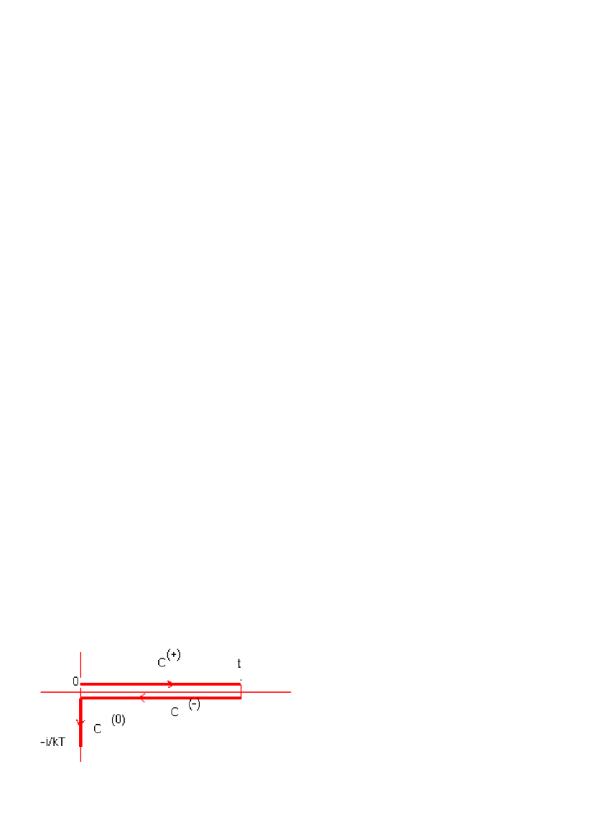
Figure 1: Complex time-path for the generating functional

The $\alpha_{i=1,2,3}$ represent states of the spin system, while the $\mathbf{\varphi}_{i=1,2,3}$ represent the bath states.  This integral can be formally written as a path integral along the path in Fig.1 with periodic boundary conditions similar to the equilibrium partition function calculations.  This functional can be calculated exactly only in few cases in particular if the Hamiltonian is quadratic.  Higher order terms can be accounted for only approximately.  This is best done through a graphical procedure such as the Feynman diagram technique.  Here we have a quadratic Hamiltonian and hence we can solve for $\mathbb{Z}$, however we will mention briefly what happens in the general case.

In our case, the bath degrees of freedom can be integrated out exactly and we can derive an exact effective action for the spin degrees of freedom. In the general case, the effective action can be derived perturbatively. From it, we will calculate the correlation functions of $\mathbf{S}$. We find

$$\mathbb{Z}\left[\mathbf{J},\mathbf{J}^{\ast}\right] = \int d\mu(\alpha_{1})\int d\mu(\alpha_{2})\int d\mu(\alpha_{3})\;\exp\left\{-\left|\alpha_{1}\right|^{2}-\left|\alpha_{2}\right|^{2}-\left|\alpha_{3}\right|^{2}\right\}$$

$$\times\int_{\alpha_{1}}^{\overline{\alpha}_{3}}d\mu(z_{1})\int_{\alpha_{3}}^{\overline{\alpha}_{2}}d\mu(z_{2})\int_{\alpha_{2}}^{\overline{\alpha}_{1}}d\mu(z_{3})\;\exp\left\{\sum_{i=1}^{3}I_{i}\left[z_{i},\overline{z}_{i},J_{i},J_{i}^{\ast}\right]\right\}\mathcal{F}\left(\mathbf{Z},\overline{\mathbf{Z}}\right)$$

where $\mathcal{F}\left(\mathbf{Z},\overline{\mathbf{Z}}\right)$ is the Feynman-Vernon functional for the spin-bath system.  It is given by

$$\ln\mathcal{F}\left(\mathbf{Z},\overline{\mathbf{Z}}\right)=\int dt\int dt^{\prime}\left[-\sum_{k}\left|\gamma_{k}\right|^{2}\overline{\mathbf{Z}}\left(t\right)\cdot G^{k}\left(t,t^{\prime}\right)\cdot\mathbf{Z}\left(t^{\prime}\right)\right],$$ (74)

where the three-vector $\mathbf{Z}$ is related to the three branches of the curve $C$, Fig. 1,

$$\mathbf{Z}=\left(\begin{array}[c]{c}z_{1}\\ -z_{2}\\ z_{3}\end{array}\right).$$ (75)

The time integrations are defined based on the path $C$:

$$t_{i} <t,t^{\prime}<t_{f}, t,t^{\prime}\in C^{(+)},C^{(-)}$$

$$t_{i} <t,t^{\prime}<t_{i}-i\beta, t,t^{\prime}\in C^{(0)}.$$

The Feynman-Vernon term is the only term which is dependent on the bath parameters.  The functions $G^{k}_{ij}\left(t,t^{\prime}\right)$, nine in total, are propagators associated with the bath oscillators.  Hence they can easily be calculated using Eq.$\left(\ref{phase}\right)$ since the oscillator part of the Hamiltonian is quadratic and the spin can be considered as the external field.  The indices $i,j=1,2,3$ relate to the branches $C^{(+)},C^{(-)},C^{(0)}$ of $C$. They are rivers

$$G_{ij}^{k}(t-t^{\prime})=\left[\begin{array}[c]{ccc}\theta\left(t-t^{\prime}\right)G_{21}^{k}+\theta\left(t^{\prime}-t\right)G_{12}^{k}&n\left(\omega_{k}\right)e^{-i\omega_{k}\left(t-t^{\prime}\right)}&\\ n\left(\omega_{k}\right)e^{\beta\omega_{k}}e^{-i\omega_{k}\left(t-t^{\prime}\right)}&\theta\left(t-t^{\prime}\right)G_{12}^{k}+\theta\left(t^{\prime}-t\right)G_{21}^{k}&\\ n\left(\omega_{k}\right)e^{\beta\omega_{k}}e^{i\omega_{k}(t+i\tau)}&G_{31}^{k}(t-\tau)&\\ \end{array}\right.$$

$$\left.\begin{array}[c]{ccc}&&n\left(\omega_{k}\right)e^{-i\omega_{k}(t+i\tau)}\\ &&G_{13}^{k}\left(t,\tau\right)\\ &&n\left(\omega_{k}\right)e^{-\omega_{k}\left(\tau-\tau^{\prime}-\frac{\beta}{2}\right)}\left[\theta\left(\tau-\tau^{\prime}\right)e^{\omega_{k}\frac{\beta}{2}}+\theta\left(\tau^{\prime}-\tau\right)e^{-\omega_{k}\frac{\beta}{2}}\right]\end{array}\right].$$ (76)

These “path-coupling” functions show that if the initial time $t_{i}$ is taken to be in the infinite past, $t_{i}\longrightarrow-\infty$, the branch $C^{(0)}$ decouples from the other two branches. rivers  This is the case where transient effects have died out.  In the rest of this paper, these transient effects will be neglected and we will concentrate only on the real-time paths $C^{(+)}$ and $C^{(-)}$.  We take account of the third branch through the assumption that initially the system is in equilibrium.  For a general potential $V$, the generating functional can be written in terms of that of a free system, $\widehat{\mathcal{H}}_{0}=\Omega a^{\dagger}a$, interacting with the bath,

$$\mathbb{Z}\left[\mathbf{J},\overline{\mathbf{J}}\right]=\exp\left\{-{i}\int_{C}dt\;V\left[\frac{\partial}{\partial J_{i}(t)},\frac{\partial}{\partial\overline{J}_{i}(t)}\right]\right\}\mathbb{Z}_{SB}\left[\mathbf{J},\overline{\mathbf{J}}\;\right].$$ (77)

$\mathbb{Z}_{SB}$ is therefore the generating functional of a particle interacting with the bath and there is no external potential.  This latter formula is valid in the general case and is the start of any perturbative calculations.   The action along the real-time trajectories is given by

$$iI_{1}^{0}={i}\int dt\left[\frac{\overset{\cdot}{\overline{z}}_{1}z_{1}-\overline{z}_{1}\overset{\cdot}{z}_{1}}{2i}-\Omega\overline{z}_{1}z_{1}\right]$$ (78)

along the path $C^{\left(+\right)}$ and by

$$iI_{2}^{0}=-i\int dt\left[\frac{\overset{\cdot}{\overline{z}}_{2}z_{2}-\overline{z}_{2}\overset{\cdot}{z}_{2}}{2i}-\Omega\overline{z}_{2}z_{2}\right]$$ (79)

along the path $C^{\left(-\right)}$, Fig. 1. At $t_{i}\rightarrow-\infty$,   the system is at equilibrium, then we can assume that the initial density matrix is thermal, with $J_{3}(t_{i})=0$.  Therefore we write that

$$\rho\left(t_{i}\right)=\frac{1}{Z(t_{i})}e^{-\beta H(t_{i})},\quad t_{i}\to-\infty$$ (80)

Then, we observe that

$$\left\langle\alpha_{1}\left|\rho(-\infty)\right|\alpha_{2}\right\rangle=\int_{\alpha_{1}}^{\overline{\alpha}_{2}}d\mu(z_{3})e^{iI_{3}^{0}\left[z_{3},\overline{z}_{3}\right]}\mathcal{F}\left(z_{3},\overline{z}_{3}\right),$$ (81)

where $I_{3}^{0}$ has the same expression as $I_{1}^{0}$ but with $t\rightarrow it$.  Hence in this case, the initial density matrix element is just another overall factor in the generating functional $\mathbb{Z}$,

$$\mathbb{Z}\left[\mathbf{J},\overline{\mathbf{J}}\;\right] = \int d\overline{\mu}(\alpha_{3})\int d\overline{\mu}(\alpha_{1})d\overline{\mu}(\alpha_{2})\left\langle\alpha_{1}\left|\rho(-\infty)\right|\alpha_{2}\right\rangle$$

$$\times\int_{\alpha_{1}}^{\overline{\alpha}_{3}}d\mu(z_{1})\int_{\alpha_{3}}^{\overline{\alpha}_{2}}\left[d\mu(z_{2})\exp\left[-\int_{C^{+}}dt\;V\left(\frac{\partial}{\partial\mathbf{J}(t)},\frac{\partial}{\partial\overline{\mathbf{J}}(t)}\right)\right]\right]$$

$$\times\exp\left\{iI_{1}^{0}\left[z_{1},\overline{z}_{1}\right]+iI_{2}^{0}\left[z_{2},\overline{z}_{2}\right]+i\int dt\left(\mathbf{J}\cdot\overline{\mathbf{Z}}+\overline{\mathbf{J}}\cdot\mathbf{Z}\right)\right\}\mathcal{F}\left(\mathbf{Z},\overline{\mathbf{Z}}\right),$$

with $\mathbf{Z}=\left(z_{1},-z_{2}\right)$ and the measure is defined by

$$d\overline{\mu}\left(\alpha\right)=d\mu\left(\alpha\right)e^{-\left|\alpha\right|^{2}}.$$ (83)

Therefore we define a new generating functional $\widehat{\mathbb{Z}}$

$$\mathbb{Z}\left[\mathbf{J},\overline{\mathbf{J}}\right]=\int d\overline{\mu}(\alpha_{3})\int d\overline{\mu}(\alpha_{1})\left[\int d\overline{\mu}(\alpha_{2})\left\langle\alpha_{1}\left|\rho(-\infty)\right|\alpha_{2}\right\rangle\times\widehat{\mathbb{Z}}\left[\mathbf{J},\overline{\mathbf{J}}\right]\right].$$

We can now adopt a different notation that takes into account the path $C$ implicitly by defining a scalar product and combine the different components into a single vector.  The generating function becomes

$$\widehat{\mathbb{Z}}\left[\mathbf{J},\overline{\mathbf{J}}\;\right] = \int d\mu(z_{1})\int d\mu(z_{2})\exp\left[-\int dtV\left(\frac{\partial}{\partial\mathbf{J}(t)},\frac{\partial}{\partial\overline{\mathbf{J}(t)}}\right)\right]$$ (84)

$$\times\exp\left\{iI^{0}\left(\mathbf{Z},\overline{\mathbf{Z}}\right)+i\int dt\left(\overline{\mathbf{Z}}\cdot\mathbf{J}+\overline{\mathbf{J}}\cdot\mathbf{Z}\right)\right\}\mathcal{F}\left(\mathbf{Z},\overline{\mathbf{Z}}\right),$$

where now the vector $\mathbf{Z}$ is defined

$$Z=\left(\begin{array}[c]{c}z_{1}\\ z_{2}\end{array}\right),$$ (85)

and the free action is

$$I^{0}=\sum_{i=i,j}\sigma^{ij}I_{j}^{0},$$ (86)

with

$$\sigma^{ij} =\left(\begin{array}[c]{cc}1&0\\ 0&-1\end{array}\right).$$ (89)

The complex scalar product is now defined by

$$\overline{\mathbf{Z}}\cdot\mathbf{J}=\sigma^{ij}\overline{z_{j}}J_{j}.$$ (90)

This notation makes it possible to take into account the closedness of the real-time path by just taking one branch of the curve $C$ and doubling the components of the dynamical variables.  The matrix $\sigma_{ij}$ plays the role of a metric.

Now we turn to some properties satisfied by the functions $G_{ij}^{k}$.  These properties are better displayed in Fourier space.  The Fourier space representation of the Feynman propagator is given by

$$G_{11}^{k}\left(\omega\right) = \int dt\;e^{i\omega t}\left(1+n\left(\omega_{k}\right)\right)\Theta\left(t\right)e^{-i\omega_{k}t}+\int dt\;e^{i\omega t}n\left(\omega_{k}\right)\theta\left(-t\right)e^{-i\omega_{k}t}$$ (91)

$$= \left(1+n\left(\omega_{k}\right)\right)\frac{i}{\omega-\omega_{k}+i\epsilon}-n\left(\omega_{k}\right)\frac{i}{\omega-\omega_{k}-i\epsilon},$$ (92)

where $\epsilon\longrightarrow 0^{+}$.  $\mathcal{P}$ stands for the principal part of the integral. For the anti-time ordered propagator, we have

$$G_{22}^{k}\left(\omega\right) = \int dte^{i\omega t}n\left(\omega_{k}\right)\Theta\left(t\right)e^{-i\omega_{k}t}+\int dte^{i\omega t}\left(1+n\left(\omega_{k}\right)\right)\Theta\left(-t\right)e^{-i\omega_{k}t}$$ (93)

$$= n\left(\omega_{k}\right)\frac{i}{\omega-\omega_{k}+i\epsilon}-\left(1+n\left(\omega_{k}\right)\right)\frac{i}{\omega-\omega_{k}-i\epsilon}.$$ (94)

For the other remaining Green functions, we have for positive $\omega$

$$G_{12}^{k}\left(\omega\right)=2\pi n\left(\omega_{k}\right)\delta\left(\omega-\omega_{k}\right),$$ (95)

and

$$G_{21}^{k}\left(\omega\right)=2\pi\left(1+n\left(\omega_{k}\right)\right)\delta\left(\omega-\omega_{k}\right).$$ (96)

These Green functions are not all independent.  We first observe that

$$G_{11}^{k}\left(\omega\right)+G_{22}^{k}\left(\omega\right)=G_{12}^{k}\left(\omega\right)+G_{21}^{k}\left(\omega\right).$$ (97)

This is an immediate result of their definition.  Moreover, the term on the l.h.s. is easily seen to be a symmetric sum of the product of two operators.  Now it is not difficult to show from the above expressions of the Green functions that we have

$$G_{11}^{k}\left(\omega\right)+G_{22}^{k}\left(\omega\right)=\left(1+2n(\omega)\right)\left[G_{21}^{k}\left(\omega\right)-G_{12}^{k}\left(\omega\right)\right].$$ (98)

The last factor on the r.h.s. is an anti-symmetric sum of two operators.  Equation $(\ref{fluct-diss-gen})$ is a statement of some form of the fluctuation dissipation theorem. martin .  These relations will be used in subsequent sections to calculate the correlation functions.  In equilibrium, when the distribution functions are the Bose-Enstein functions

$$1+2n(\omega)=\coth\frac{\beta\omega}{2}$$ (99)

and equation $(\ref{fluct-diss-gen})$ gives the usual from of the fluctuation-dissipation theorem.

5 Normal Mode Analysis

In this section we follow Lyberatos, Berkov and Chantrell lyberatos and couple the normal modes of the spin system (also called collective field) to the harmonic oscillators of the bath.   This method has also been recently used by Safonov and Bertram to calculate correlation functions of the magnetization in thin films. safonov  In this section, we show how their correlation functions for the collective field follow from the microscopic model treated here.  The results in this section will be used in the next section to find the correlation functions of the magnetization in the general case.

First we find the collective degrees of freedom $c$ and $c^{\dagger}$ from the magnetization:

$$a = uc+vc^{\dagger}$$ (100)

$$a^{\dagger} = vc+uc^{\dagger}$$

where $u$ and $v$ are real.  We require that

$$\left[c,c^{\dagger}\right]=1.$$ (101)

This implies that

$$u^{2}-v^{2}=1.$$ (102)

Therefore, we can write for some $\theta$,

$$u = \cosh\theta$$ (103)

$$v = \sinh\theta.$$

If we set,

$$\omega_{0}^{2}=\Omega^{2}-\frac{K^{2}}{4},$$ (104)

we find that the coefficients of the transformation Eq.$\left(\ref{transf}\right)$,

$$u = \sqrt{\frac{\Omega+\omega_{0}}{2\omega_{0}}},$$ (105)

$$v = -\sqrt{\frac{\Omega-\omega_{0}}{2\omega_{0}}}.$$

In this collective coordinates, the spin Hamiltonian becomes diagonal,

$$\mathcal{H}_{S}=\omega_{0}c^{\dagger}c.$$ (106)

Now the interaction term between the bath and the spin is taken of the form

$$\widehat{\mathcal{H}}_{SR}=-\sum_{k}\left(\gamma_{k}c^{\dagger}b_{k}+\gamma_{k}^{\ast}b_{k}^{\dagger}c\right).$$ (107)

The generating functional for this system is then calculated in Fourier space with the help of the Green functions stated in the last section.  We find that

$$\widehat{\mathbb{Z}}\left[\,\overline{\mathbf{J}},\mathbf{J}\right] = \int d\mu\left(\overline{z}_{1},z_{1}\right)\int d\mu\left(\overline{z}_{2},z_{2}\right)\exp\left\{-\int\frac{d\omega}{2\pi}\;\left[\;\overline{\mathbf{Z}}\cdot\mathcal{A}\cdot\mathbf{Z}+\overline{\mathbf{J}}\cdot\mathbf{Z}+\mathbf{J}\cdot\overline{\mathbf{Z}}\;\right]\right\}$$ (108)

$$= \frac{1}{\det\mathcal{A}}\exp\left\{-\int\frac{d\omega}{2\pi}\;\overline{\mathbf{J}}\cdot\mathcal{A}^{-1}\cdot\mathbf{J}\right\}$$

where $\mathbf{Z}=\left(z_{1},z_{2}\right)$ and $\mathbf{J}=\left(J_{1},J_{2}\right)$ are two-component vectors. The matrix $\mathcal{A}$ is

$$\mathcal{A}_{ij}=\left[\begin{array}[c]{cc}i\left(\omega_{0}-\omega\right)+\Pi_{11}\left(\omega\right)&\Pi_{12}\left(\omega\right)\\ \Pi_{21}\left(\omega\right)&-i\left(\omega_{0}-\omega\right)+\Pi_{22}\left(\omega\right)\end{array}\right].$$ (109)

The $\Pi_{ij}$ terms are due to the interaction of the system with the bath. They depend on the density of states of the bath $\lambda(\omega)$ and the coupling constants.  For a general bath, the $Pi_{11}$ element is given

$$\Pi_{11}\left(\omega\right) = \sum_{k}\left|\gamma_{k}\right|^{2}G_{11}^{k}\left(\omega\right)$$ (110)

$$= i\int\frac{d\omega_{k}}{\pi}\pi\lambda\left(\omega_{k}\right)\left|\gamma\left(\omega_{k}\right)\right|^{2}\left[\frac{1+n\left(\omega_{k}\right)}{\omega-\omega_{k}+i\epsilon}-\frac{n\left(\omega_{k}\right)}{\omega-\omega_{k}-i\epsilon}\right].$$ (111)

The remaining matrix elements are calculated similarly. If now, we assume that the bath parameters satisfy the condition

$$\pi\lambda\left(\omega_{k}\right)\left|\gamma\left({\omega_{k}}\right)\right|^{2}=\alpha\;\;\;\;\;\;\left(\omega_{k}>0\right),$$ (112)

where $\alpha$ is a constant, we find that the interaction with the bath induces the following coefficients,

$$\Pi_{11}\left(\omega\right) = \,\alpha\left(1+2n(\omega)\right)$$ (113)

$$\Pi_{22}\left(\omega\right) = \Pi_{11}\left(\omega\right)$$ (114)

$$\Pi_{12}\left(\omega\right) = 2\alpha n\left(\omega\right)$$ (115)

$$\Pi_{21}\left(\omega\right) = 2\alpha\left(1+n\left(\omega\right)\right).$$ (116)

The correlation functions of the magnetization are related to the inverse elements of the matrix $\mathcal{A}$.  A calculation of the inverse matrix gives

$$\mathcal{A}^{-1}=\frac{1}{\mathcal{D}}\left[\begin{array}[c]{cc}i\left(\omega_{0}-\omega\right)+\alpha\left(1+2n(\omega)\right)&-2\alpha n\left(\omega\right)\\ -2\alpha\left(1+n\left(\omega\right)\right)&-i\left(\omega_{0}-\omega\right)+\alpha\left(1+2n(\omega)\right)\end{array}\right].$$ (119)

where $\mathcal{D}$ is the determinant

$$\mathcal{D}=\det\mathcal{A}=\left(\omega_{0}-\omega\right)^{2}+\alpha^{2}.$$ (120)

After solving for the generating functional in terms of the external sources, we can expand it around the point $\mathbf{J}=\mathbf{J}^{\ast}=0$ to get all the required correlation functions.  In this case, we can solve for $\widehat{\mathbb{Z}}\left[\,\overline{\mathbf{J}},\mathbf{J}\right]$ exactly since the full Hamiltonian is quadratic.   The correlation functions are now found by differentiations with respect to $\overline{\mathbf{J}}$ and/or $\mathbf{J}$. For $t>t^{\prime}$, we have for the correlation function of the collective operator $c$

$$\left\langle c^{\dagger}(t)c(t^{\prime})\right\rangle=i\frac{\partial}{\partial J_{2}(t)}\frac{\partial}{\partial\overline{J}_{1}(t^{\prime})}\left.\mathbb{W}\left[\;\overline{\mathbf{J}},\mathbf{J}\right]\right|_{\mathbf{J}=\overline{\mathbf{J}}=0}$$ (121)

where

$$\mathbb{W}\left[\,\overline{\mathbf{J}},\mathbf{J}\right]=i\int\frac{d\omega}{2\pi}\,\overline{J}_{i}\left(\omega\right)\mathcal{A}_{ij}^{-1}\left(\omega\right)J_{j}\left(\omega\right)$$ (122)

All correlation functions of three operators or more are zero since the Hamiltonian is quadratic.  The above correlation function is therefore related to the matrix element, $\mathcal{A}^{-1}_{12}$.  At high temperature, i.e., $\beta\rightarrow 0\left(\omega<<kT\right)$

$$\mathcal{A}_{12}^{-1}(\omega) = -\frac{2\alpha n\left(\omega\right)}{\left(\omega_{0}-\omega\right)^{2}+\alpha^{2}}$$ (123)

$$= \frac{-2\alpha kT}{\omega}\frac{1}{\left(\omega_{0}-\omega\right)^{2}+\alpha^{2}}$$ (124)

In real time, we have

$$\mathbb{W}\left[\,\overline{J},J\right]=i\int{dt}\int dt^{\prime}\,\overline{J}_{i}\left(t\right)\mathcal{A}_{ij}^{-1}\left(t-t^{\prime}\right)J_{j}\left(t^{\prime}\right),$$ (125)

hence, the two-point correlation function of the field $c$ associated with the $1-2$ component of the path $C$ is

$$\left\langle c^{\dagger}(t)c(t^{\prime})\right\rangle=2\alpha\int\frac{d\omega}{2\pi}e^{-i\omega\left(t-t^{\prime}\right)}\frac{n\left(\omega\right)}{\left(\omega_{0}-\omega\right)^{2}+\alpha^{2}}.$$ (126)

Similarly, we can find the corresponding $2-1$ component of the correlation function,

$$\left\langle c(t^{\prime})c^{\dagger}(t)\right\rangle=2\alpha\int\frac{d\omega}{2\pi}e^{-i\omega\left(t-t^{\prime}\right)}\frac{1+n\left(\omega\right)}{\left(\omega_{0}-\omega\right)^{2}+\alpha^{2}}.$$ (127)

From these last two correlation function, we get the classical correlation function of $c$,

$$\frac{1}{2}\left\langle c^{\dagger}(t)c(t^{\prime})+c(t^{\prime})c^{\dagger}(t)\right\rangle=\alpha\int\frac{d\omega}{2\pi}e^{-i\omega\left(t-t^{\prime}\right)}\frac{1+2n\left(\omega\right)}{\left(\omega_{0}-\omega\right)^{2}+\alpha^{2}}.$$ (128)

Now we observe that if we take the limits $\alpha\longrightarrow 0$ and $t^{\prime}\longrightarrow t$, we recover the expectation value of the occupation number $\widehat{n}=cc^{\dagger}$,

$$\langle\widehat{n}\left(\omega\right)\rangle=1+n\left(\omega\right).$$ (129)

To get this limit, we have used the fact that

$$\frac{1}{\pi}\frac{\alpha}{\omega^{2}+\alpha^{2}}\longrightarrow\delta\left(\omega\right)\;\;\;\;\text{as}\;\;\;\alpha\longrightarrow 0.$$

We also note that in this limit, we have

$$\langle c^{{\dagger}}c+cc^{{\dagger}}\rangle=1+2n\left(\omega\right),$$ (130)

and

$$\langle[c(t),c^{{\dagger}}(t)]\rangle=1.$$ (131)

This shows that the commutations relations and the FDT are satisfied at all times $t$.

Since we are close to equilibrium and $\alpha$ is small, the power spectrum will be picked near $\omega=\omega_{0}$.  Therefore, this is also equivalent to having a Langevin equation with random forces F such that haken

$$\overset{.}{c}=-(i\omega_{0}+\alpha)c+F\left(t\right)$$ (132)

and

$$\left\langle\left\{F^{\dagger}\left(t\right),F\left(t^{\prime}\right)\right\}\right\rangle=2\alpha kT\delta\left(t-t^{\prime}\right).$$ (133)

Within this approximation, we recover the correlation functions of Safonov-Bertram, Eq.$\left(2.14\right)$ in Ref. safonov .

$$\left\langle c^{\dagger}(t)c(0)\right\rangle=\int\frac{d\omega}{2\pi}\frac{2\alpha kT}{\omega_{0}}\frac{e^{-i\omega t}}{\left(\omega_{0}-\omega\right)^{2}+\alpha^{2}}.$$ (134)

To get the correlation functions of the magnetization $\mathbf{S}$, we first use the linear transformation, Eq. $\left(\ref{transf}\right)$, to write $S_{x}$ and $S_{y}$ in terms of the collective operators $c$ and $c^{{\dagger}}$.  This result will be deduced in the next section from the exact treatment of the general asymmetric case and without recourse to the rotating wave approximation as was done in Ref. safonov .

6 White and Colored Noise: LLG and Other Solutions

One could compute the correlation functions for the original variables from the $cc^{\dagger}$ correlation functions, by inverting the Bogoliubov transformation (100). However, in this section, we will repeat the computation directly in terms of original magnetization component variables,

$$\widehat{S}_{x} = \frac{1}{2}\left(a+a^{\dagger}\right),$$ (135)

$$\widehat{S}_{y} = \frac{1}{2i}\left(a-a^{\dagger}\right)\;.$$ (136)

Writing the generating functional $\overline{\mathbb{Z}}$ in terms of them is trivial, but performing the Gaussian integration is more complicated, since we will have to invert a $4\times 4$ matrix.  We couple the magnetization to an external time dependent magnetic field $\mathbf{F}$

$$\widehat{\mathcal{H}}_{e}=-\mathbf{F}\cdot\widehat{\mathbf{S}}.$$ (137)

As we have seen in the previous section, in the generating functional approach, we double the components of $\mathbf{S}$ and that implies doubling of the external field $\mathbf{F}$.  Therefore the interaction term becomes

$$\widehat{H}_{e}=-\mathbf{F}_{1}\cdot\mathbf{S}_{1}+\mathbf{F}_{2}\cdot\mathbf{S}_{2}.$$ (138)

The results for this Hamiltonian can be derived from those already found in the previous section. The bath contributes a term of the following form to the effective action

$$S_{eff}\left(\mathbf{S}_{1},\mathbf{S}_{2}\right) = \left.\int\frac{d\omega}{2\pi}\left|\gamma_{k}\right|^{2}G_{11}^{k}\left(\omega\right)\left[S_{1,x}^{2}+S_{1,y}^{2}+i\overline{S}_{1,x}S_{1,y}-i\overline{S}_{1,y}S_{1,x}\right]\right.$$

$$-\int\frac{d\omega}{2\pi}\left|\gamma_{k}\right|^{2}G_{22}^{k}\left(\omega\right)\left[S_{2,x}^{2}+S_{2,y}^{2}+i\overline{S}_{2,x}S_{2,y}-i\overline{S}_{2,y}S_{2,x}\right]$$

$$+\int\frac{d\omega}{2\pi}\left|\gamma_{k}\right|^{2}G_{21}^{k}\left(\omega\right)\left[\overline{S}_{2,x}S_{1,x}+\overline{S}_{2,y}S_{1,y}+i\overline{S}_{2,x}S_{1,y}-i\overline{S}_{2,y}S_{1,x}\right]$$

$$+\left.\int\frac{d\omega}{2\pi}\left|\gamma_{k}\right|^{2}G_{12}^{k}\left(\omega\right)\left[\overline{S}_{1,x}S_{2,x}+\overline{S}_{1,y}S_{2,y}+i\overline{S}_{1,x}S_{2,y}-i\overline{S}_{1,y}S_{2,x}\right]\right\}$$

where the bar denotes the complex conjugate integration variables and $S_{1}$ $\left(S_{2}\right)$ is the component along the path $C^{(+)}\left(C^{(-)}\right)$, Fig. 1. Next, we define two new vectors $\mathbf{S}$ and $\mathbf{D}$,

$$\mathbf{S} = \frac{1}{2}\left(\mathbf{S}_{1}+\mathbf{S}_{2}\right),$$ (140)

$$\mathbf{D} = \mathbf{S}_{1}-\mathbf{S}_{2}.$$ (141)

Similarly, we define

$$\mathbf{F}_{d} = \mathbf{F}_{1}-\mathbf{F}_{2},$$ (142)

$$\mathbf{F}_{a} = \frac{1}{2}\left(\mathbf{F}_{1}+\mathbf{F}_{2}\right).$$ (143)

Finally, we make another definition. We define four-vectors $\mathbf{U}$ and $\mathbf{F}$

$$\mathbf{U} = \left(S_{x},S_{y},D_{x},D_{y}\right),$$ (144)

$$\mathbf{F} = \left(\mathbf{F}_{d},\mathbf{F}_{a}\right),$$ (145)

and write the generating functional in terms of these four-vectors along the path $C^{\left(+\right)}$ only.  Since $\mathbf{U}\left(t\right)$ is real, then we have

$$\overline{U}\left(\omega\right)=U\left(-\omega\right),$$

and hence we should constrain the fourier integration to positive frequencies only.  The bath-independent part of the Hamiltonian then gives the following contribution to the phase of $\widehat{\mathbb{Z}}$,

$$iI_{1}-iI_{2}=-\int_{0}^{\infty}\frac{d\omega}{\pi}\overline{U}_{i}\left(\omega\right)\mathcal{A}_{ij}^{(0)}\left(\omega\right)U_{j}\left(\omega\right),$$ (146)

where the matrix $\mathcal{A}^{(0)}$ is, in Fourier space,

$$\mathcal{A}_{ij}^{(0)}=\left[\begin{array}[c]{cccc}0&0&iA&-\omega\\ 0&0&\omega&iB\\ iA&-\omega&0&0\\ \omega&iB&0&0\end{array}\right].$$ (147)

Again, it is the inverse of the full matrix $\mathbf{\mathcal{A}}=\mathbf{\mathcal{A}}^{(0)}+\mathbf{\mathcal{A}}^{\text{int}}$, that is needed to determine the correlation functions of the magnetization where  $\mathbf{\mathcal{A}}^{\text{int}}$ is the part that is due to the interaction with the bath. The determinant of $\mathbf{\mathcal{A}}$ determines the natural frequency of the system and any broadening due to interactions.  The determinant of the free part is

$$\mathcal{D}_{0}=\left(\omega_{0}^{2}-\omega^{2}\right)^{2},$$ (148)

where

$$\omega_{0}^{2}=AB,$$ (149)

is the ferro-magnetic resonance (FMR) frequency of the system.  The calculation of the matrix $\mathbf{\mathcal{A}}$ is done along the same lines as in the normal mode solution.

To recover dissipative behavior in the spin sub-system, we take the continuum limit in the number of oscillator modes.  This limit guarantees that the probability of acquiring back any energy lost to the bath is zero.  Because of the interaction with the bath, we expect that there will be a shift in the energy of the spin system accompanied by dissipation.

An explicit computation shows that in the continuum limit, i.e. converting the sum over $k$ in an integral over the frequencies involving the density of states $\lambda(\omega_{k})$

$$\lambda(\omega_{k})=\frac{dk}{d\omega_{k}}\;,$$ (150)

the correlation functions can be expressed in terms of the functions $L_{r}$ and $L_{i}$ :

$$L_{r}\left(\omega\right) = -i\int_{0}^{\infty}\frac{d\omega_{k}}{\pi}\;\pi\lambda\left(\omega_{k}\right)\left|\gamma\left(\omega_{k}\right)\right|^{2}(G_{11}^{k}-G_{22}^{k})\left(\omega_{k}\right),$$ (151)

$$L_{i}\left(\omega\right) = 2\int_{0}^{\infty}\frac{d\omega_{k}}{\pi}\;\pi\lambda\left(\omega_{k}\right)\left|\gamma\left(\omega_{k}\right)\right|^{2}(G_{12}^{k}-G_{21}^{k})\left(\omega_{k}\right).$$ (152)

Using the definitions of the Green functions, we find

$$L_{r}\left(\omega\right) = 2\mathcal{P}\int_{0}^{\infty}\frac{d\omega_{k}}{\pi}\pi\lambda\left(\omega_{k}\right)\left|\gamma\left(\omega_{k}\right)\right|^{2}\frac{1}{\omega-\omega_{k}}\;,$$ (153)

$$L_{i}\left(\omega\right) = -2\pi\lambda\left(\omega\right)\left|\gamma\left(\omega\right)\right|^{2}\theta(\omega)\;.$$ (154)

Counter-terms are needed to cancel ultraviolet divergences in $L_{r}$.  For simplicity, we will assume that this is done via suitable subtractions. The effect of $L_{r}$ is a redefinition of the given coefficients $A$ and $B$.  This redefinition in principle changes the oscillation frequency. However, for a passive path, one neglects $L_{r}(\omega)$ and thus the frequency shift. In this approximation the coefficients $A$ and $B$ are kept unnormalized and all the physics is contained in $L_{i}(\omega)$. There is a subtlety here, since the expression (154) is not antisymmetric, whereas it has to be antisymmetric due to general properties of correlation functions (see appendix for a discussion). Therefore $L_{i}(\omega)$ has to be antisymetrized. By noticing that $|\gamma(\omega)|^{2}$ is even in $\omega$ and extending $\lambda(\omega)$ to negative $\omega<0$ with a negative sign, the final result can be written in the form

$$\mathcal{A}=\left[\begin{array}[c]{cccc}0&0&iA-\Delta(\omega)&-\omega\\ 0&0&\omega&iB-\Delta(\omega)\\ iA+\Delta(\omega)&-\omega&\pi\lambda\left(\omega\right)\left|\gamma\left(\omega\right)\right|^{2}\left(1+2n\left(\omega\right)\right)&0\\ \omega&iB+\Delta(\omega)&0&\pi\lambda\left(\omega\right)\left|\gamma\left(\omega\right)\right|^{2}\left(1+2n\left(\omega\right)\right)\end{array}\right],$$ (155)

where $\Delta(\omega)$ is the odd function

$$\Delta\left(\omega\right) = \frac{-L_{i}\left(\omega\right)+L_{i}\left(-\omega\right)}{2}=\pi\lambda(\omega)|\gamma(\omega)|^{2}\;.$$ (156)

The determinant of this matrix is given by

$$\det\mathcal{A}=\mathcal{D}\left(\omega\right) = \left[\omega_{0}^{2}-\omega^{2}-\Delta\left(\omega\right)^{2}\right]^{2}+\left[\Delta\left(\omega\right)\left(A+B\right)\right]^{2},$$ (157)

We also observe that for the functional integral to converge, we must have

$$\pi\lambda\left(\omega\right)\left|\gamma\left(\omega\right)\right|^{2}\left(1+2n(\omega)\right)>0.$$

This requires that the function $L_{i}\left(\omega\right)$ when extended to negative frequencies be an odd function which is consistent with the statement before Eq.$(\ref{matrix})$.

To calculate the correlation functions, we need first to calculate the inverse matrix of $\mathcal{A}$.  The cofactors needed for the correlation functions of the different components of the magnetization are for small couplings to the bath

$$c_{11} = -\pi\lambda\left(\omega\right)\left|\gamma\left(\omega\right)\right|^{2}\left(1+2n({\omega})\right)\left[B^{2}+\omega^{2}+\Delta\left(\omega\right)^{2}\right],$$ (158)

$$c_{12} = i\pi\lambda\left(\omega\right)\left|\gamma\left(\omega\right)\right|^{2}\left(1+2n({\omega})\right)\left[\left(A+B\right)\omega\right],$$ (159)

$$c_{22} = -\pi\lambda\left(\omega\right)\left|\gamma\left(\omega\right)\right|^{2}\left(1+2n({\omega})\right)\left[A^{2}+\omega^{2}+\Delta\left(\omega\right)^{2}\right],$$ (160)

$$c_{12} = -c_{21}=i\pi\lambda\left(\omega\right)\left|\gamma\left(\omega\right)\right|^{2}\left(1+2n({\omega})\right)\left[\left(A+B\right)\omega\right].$$ (161)

As will be seen below, the $c_{11}\;\left(c_{22}\right)$ co-factor of the matrix $\mathcal{A}$ is associated with the $xx\;\left(yy\right)-$component of the magnetization while $c_{12}$ is related to the $xy-$component.

Correlation Functions

Next, we use these cofactors to calculate the correlation functions of the magnetization.

For a general operator $\mathcal{O}$, the average of the anti- commutator $\left\{\mathcal{O}(t),\mathcal{O}(t^{\prime})\right\}$ is found by differentiation of $\mathbb{W}\left[\mathbf{F}_{a},\mathbf{F}_{d}\right]$ with respect to $\mathbf{F}_{d}$,

$$\frac{1}{2}\langle\mathcal{O}\left(t\right)\mathcal{O}\left(t^{\prime}\right)+\mathcal{O}\left(t^{\prime}\right)\mathcal{O}\left(t\right)\rangle = -i\frac{\delta^{2}\mathbb{W}\left[\mathbf{F}_{a},\mathbf{F}_{d}\right]}{\delta\mathbf{F}_{d}\left(t\right)\delta\mathbf{F}_{d}\left(t^{\prime}\right)}$$ (162)

Applying this procedure to the components of the magnetization, we find that for the $x-$component

$$\frac{1}{2}\langle S_{x}(t)S_{x}(0)+S_{x}(0)S_{x}(t)\rangle=\int\frac{d\omega}{2\pi}\cos\omega t\;\frac{c_{11}\left(\omega\right)}{\mathcal{D}\left(\omega\right)}.$$ (163)

From Eq. $(\ref{co11})$, we then obtain

$$C_{xx}(t) = \int\frac{d\omega}{2\pi}\cos(\omega t)\left[1+2n({\omega})\right]\pi\lambda\left(\omega\right)\left|\gamma\left(\omega\right)\right|^{2}\;\frac{\left(\omega^{2}+B^{2}\right)+\Delta^{2}}{\mathcal{D}\left(\omega\right)}.$$ (164)

Now, we show how for different choices of the function $L_{i}\left(\omega\right)$, we can recover the LLG result and other oscillator-type correlation functions.

6.0.1 Case 1 :   LLG

If we assume that the bath is defined such that

$$\pi\lambda\left(\omega\right)\left|\gamma\left(\omega\right)\right|^{2}=\alpha\omega,$$ (165)

i.e., $L_{i}\left(\omega\right)$ is odd. Then in the limit of high temperature, $\beta\rightarrow 0$, the correlation function for the $xx$-component takes the simple form

$$C_{xx}(t) = 2\alpha kT\int\frac{d\omega}{2\pi}\cos(\omega t)\;\left[\frac{\left(1+\alpha^{2}\right)\omega^{2}+B^{2}}{\left[\left(1+\alpha^{2}\right)\omega^{2}-\omega_{0}^{2}\right]^{2}+\left[\alpha\omega\left(A+B\right)\right]^{2}}\right].$$ (166)

This is the result that coincides with that derived from LLG. smith ; rebei  This case also corresponds to a white noise solution.rebei  Moreover, we observe that the condition on the bath that gives LLG is similar to the one that gave the harmonic oscillator solution, Eq.$\left(\ref{harmonic}\right)$.  In both cases the spectral density is linear in frequency.grabert

6.0.2 Case 2 :   Coherent Oscillator

This case is similar to the normal mode result.  We call it coherent oscillator because this case gives correlation functions similar to those of the collective operator $c$ in the normal mode analysis.  Here we choose $L_{i}(\omega)$ such that

$$\pi\lambda\left(\omega\right)\left|\gamma\left(\omega\right)\right|^{2}=\alpha,\;\;\;\;\omega>0.$$ (167)

This is the same choice as in the previous section. For $\beta\rightarrow 0$, we get the following expression for the $xx$-component of the correlation functions

$$C_{xx}(t)=2\alpha kT\;\int\frac{d\omega}{2\pi}\cos(\omega t)\;\left(\frac{1}{\omega}\right)\left[\frac{B^{2}+\omega^{2}+\alpha^{2}}{\left[\omega^{2}-\omega_{0}^{2}\right]^{2}+2\alpha^{2}\left(\omega^{2}+\omega_{0}^{2}\right)+\alpha^{4}}\right].$$ (168)

The normal mode result is easily seen to follow by setting $A=B$ in the correlation functions and $(1/\omega)$ by $(1/\omega_{0})$ . This result has been obtained before by Safonov and Bertram.safonov However without this latter approximation, this model corresponds to a case of colored noise.rebei  As $\omega\rightarrow 0$, the integral diverges.  Therefore at small $\omega$, the approximation in Eq. $(\ref{approx})$ is not applicable: $L_{i}(\omega)-L_{i}(-\omega)$ cannot be a constant but, for consistency with antisymmetry and analyticity, must vanish with $\omega$ at $\omega\to 0$.

7 Conclusion

Starting from simple quantum models which only differ in how the spin couples to the bath, we have been able to derive variant correlation functions for the magnetization close to equilibrium.  We have limited ourselves only to linear-type couplings.  Depending on the coupling and the density of states of the bath, we showed how to obtain different types of correlation functions including the classical LLG result.  First, we showed that the typical harmonic oscillator correlation functions are recovered only if the $S_{x}$ component of the magnetization is coupled to the bath oscillators.  Next, we coupled the normal modes of the spin to those of the bath and this allowed us to get the correlation functions of the collective field which is the starting point of the work of Safonov and Bertram.  We were also able to use this special coupling to derive a more general type of correlation functions without recourse to any approximations such as the rotating wave approximation.  These correlation functions are for a general linear coupling between the bath and the magnetization depend on the coupling constant $\gamma$ and the density of states of the bath system, $\lambda(\omega)$.  For the $S_{x}S_{x}$-correlation function we find,

$$C_{xx}(t)=\int\frac{d\omega}{2\pi}\left[1+2n(\omega)\right]\Delta\left(\omega\right)\cos(\omega t)\left[\frac{\omega^{2}+B^{2}+\Delta\left(\omega\right)^{2}}{\left(\omega_{0}^{2}-\omega^{2}-\Delta\left(\omega\right)^{2}\right)^{2}+\left[\Delta\left(\omega\right)\left(A+B\right)\right]^{2}}\right].$$ (169)

Similarly for the $S_{y}S_{y}$-correlation function, we have

$$C_{yy}(t)=\int\frac{d\omega}{2\pi}\left[1+2n(\omega)\right]\Delta\left(\omega\right)\cos(\omega t)\left[\frac{\omega^{2}+A^{2}+\Delta\left(\omega\right)^{2}}{\left(\omega_{0}^{2}-\omega^{2}-\Delta\left(\omega\right)^{2}\right)^{2}+\left[\Delta\left(\omega\right)\left(A+B\right)\right]^{2}}\right],$$ (170)

and finally for the $S_{x}S_{y}$-correlation function, the correlation function is

$$C_{xy}(t) = \int\frac{d\omega}{2\pi}\left[1+2n(\omega)\right]\Delta\left(\omega\right)\sin(\omega t)\left[\frac{\omega\left(A+B\right)}{\left(\omega_{0}^{2}-\omega^{2}-\Delta\left(\omega\right)^{2}\right)^{2}+\left[\Delta\left(\omega\right)\left(A+B\right)\right]^{2}}\right],$$ (171)

where

$$\Delta\left(\omega\right)=\pi\lambda\left(\omega\right)\left|\gamma\left(\omega\right)\right|^{2}.$$ (172)

The LLG solution was obtained for a special type of density of states and coupling to the bath.  The same condition was also obtained in Ref. rebei where in addition we were able to show that this choice gives the white noise character in the stochastic formulation .  The normal mode solutions are however in general with memory.  The assumption that damping is constant close to the FMR frequency makes the equations of motion Markovian.peier  The damping in the cases treated here is independent of the symmetries of the Hamiltonian spin system, the reason being that the dissipation kernel only depends on the coupling with the bath and the bath properties, but not on the spin Hamiltonian.  For couplings other than linear, the damping is expected to depend on the symmetries of the full Hamiltonian, but, again, not at the leading order in perturbation theory.  The point is that for non-linear coupling, the effective Hamiltonian and therefore the correlation functions have to be computed perturbatively in terms of Feynman diagrams; in particular the spin propagator will enter in higher order computations and since the spin propagator depends on the symmetry of the spin Hamiltonian, which could be isotropic ($A=B$) or not ($A\neq B$), we will have different results for $A=B$ and $A\neq B$.   This does not happen at leading order in the non-linear case, and does not happen at all orders in the linear case, where the exact result is available.

One last word about the non-equilibrium machinery used here to derive the above correlation functions: this choice of method allows us to go beyond the equilibrium formulation, and in particular to show that a generalized fluctuation-dissipation theorem (98) holds true even if the distribution functions are not exactly the Bose-Einstein ones.  In principle, an analysis of this system when the distribution functions present strong differences from the thermal one is also possible in the general formalism we discussed here. However, such a strongly out of equilibrium analysis would require further study and it is outside the scope of the present paper.

Appendix

Here we briefly show how the correlation functions derived in the main text can be derived using the equilibrium imaginary time formalism orland and without going to the coherent state representation. This is an equilibrium consistency check for our non-equilibrium computation.

The basic idea in the equilibrium computation is to invoke the fluctuation-dissipation theorem (which is not assumed in the non-equilibrium computation) in order to derive the fluctuations from the dissipation, i.e. from the spectral density. The fluctuation-dissipation theorem says that in equilibrium the symmetric correlation functions can be written in terms of the spectral densities $\rho^{ij}(\omega)$ as

$$<\{S^{i}(t),S^{j}(0)\}>=\int d\omega\;e^{i\omega t}\;\coth\frac{\beta\omega}{2}\;\rho^{ij}(\omega)\;,$$ (173)

where $i$ and $j$ denote the indices $x$ and $y$ respectively. From this definition it is immediate to see that the spectral densities must satisfy the relationships

$$\rho^{ij}(\omega)^{*}=\rho^{ji}(\omega),\quad\rho^{ij}(\omega)=-\rho^{ji}(-\omega).$$ (174)

In particular, $\rho^{xx}$ and $\rho^{yy}$ are real and antisymmetric:

$$\rho^{ii}(\omega)^{*}=\rho^{ii}(\omega),\quad\rho^{ii}(\omega)=-\rho^{ii}(-\omega).$$ (175)

Thus, one can extract the spectral densities $\rho^{ii}(\omega)$ from the spectral representation of the retarded self-energy,

$$D_{R}^{ij}(\omega)=\int d\omega^{\prime}\;\frac{\rho^{ij}(\omega^{\prime})}{\omega^{\prime}-\omega+i\varepsilon}$$ (176)

by taking the imaginary part:

$$\rho^{ii}(\omega)=-\frac{1}{\pi}\mbox{ Im }D_{R}^{ii}(\omega)\;.$$ (177)

Moreover, due to the behavior of the theory under time reflections $t\to-t$,

$$<\{S^{x}(t)\,,\,S^{y}(0)\}>=-<\{S^{x}(-t)\,,\,S^{x}(0)\}>$$ (178)

we have that $\rho^{xy}(\omega)$ and $\rho^{yx}(\omega)$ are imaginary and symmetric:

$$\rho^{ij}(\omega)^{*}=-\rho^{ij}(\omega),\quad\rho^{ij}(\omega)=\rho^{ij}(-\omega),\quad i\neq j$$ (179)

As a consequence, the $\rho^{ij}(\omega),\ i\neq j$ spectral densities can be extracted from the real part of the retarded self-energy:

$$\rho^{ij}(\omega)=\frac{i}{\pi}\mbox{ Re }D_{R}^{ij}(\omega),\quad i\neq j$$ (180)

In order to compute the retarded propagators, one has to compute the Euclidean effective action obtained by integrating out the bath degrees of freedom in the Euclidean functional integral

$$e^{-S^{E}_{eff}(S^{i})}=\int[db_{k}^{*}db_{k}]\exp\left[-\int_{0}^{\beta}d\tau\;L^{E}(S^{i},b_{k},b_{k}^{*})\right]$$ (181)

where

$$L^{E}(S^{i},b_{k},b_{k}^{*})=L^{E}_{S}(S^{i})+L^{E}_{R}(b_{k},b^{*}_{k})+L^{E}_{SR}(S^{i},b_{k},b_{k}^{*}),$$ (182)

with

$$L^{E}_{S}(S^{i}) = S^{x}i\partial_{\tau}S^{y}+\frac{1}{2}A(S^{x})^{2}+\frac{1}{2}B(S^{y})^{2},$$ (183)

$$L^{E}_{R}(b_{k},b_{k}^{*}) = \sum_{k}b^{*}_{k}(\partial_{\tau}-\omega_{k})b_{k},$$ (184)

$$L^{E}_{SR}(S^{i},b_{k},b_{k}^{*}) = \sum_{k}b_{k}^{*}\gamma_{k}S_{-}+S_{+}\gamma_{k}^{*}b_{k}.$$ (185)

Since the integration on $b_{k}$ and $b_{k}^{*}$ is Gaussian, $S_{eff}$ can be computed exactly and is quadratic in the spin fields:

$$S^{E}_{eff}(S^{i})=\int_{0}^{\beta}d\tau\int_{0}^{\beta}d\tau^{\prime}\;\frac{1}{2}\;S^{i}(\tau)\;D_{ij}^{E}(\tau-\tau^{\prime})\;S^{j}(\tau^{\prime}).$$ (186)

The Euclidean propagator is easily obtained in the Matsubara formulation by inverting the 2x2 matrix

$$D_{E}^{-1}(\omega_{n})=\begin{pmatrix}A&\omega_{n}\cr-\omega_{n}&B\end{pmatrix}+\begin{pmatrix}\Pi_{E}(\omega_{n})&0\cr 0&\Pi_{E}(\omega_{n})\end{pmatrix}$$ (187)

where the first matrix is the inverse free propagator and the second matrix is the self-energy matrix (to be compared with the real time result Eq. (110))

$$\Pi_{E}(\omega_{n})=2\sum_{k}|\gamma_{k}|^{2}G_{E}^{k}(\omega_{n})$$ (188)

and where $\omega_{n}=2\pi nT,\ n=0,\pm 1,\pm 2,\dots$ are the Matsubara frequencies. The inversion is trivial.  The retarted propagator can be obtained with an analytic continuation $\omega_{n}\to i\omega$:

$$D_{R}(\omega)=\frac{1}{\mathcal{D}(\omega)}\begin{pmatrix}B+\Pi_{R}(\omega)&-i\omega\cr i\omega&A+\Pi_{R}(\omega)\end{pmatrix}$$ (189)

where $\mathcal{D}(\omega)$ is the determinant

$$\mathcal{D}(\omega)=\omega_{0}^{2}-\omega^{2}+(A+B)\Pi_{R}(\omega)+\Pi_{R}^{2}(\omega)$$ (190)

In order to compute real and imaginary parts, it is convenient to split

$$\Pi_{R}(\omega)=\mbox{ Re }\Pi(\omega)+i\mbox{ Im }\Pi(\omega)$$ (191)

and to introduce the real quantities

$$\tilde{A}(\omega)=A+\mbox{ Re }\Pi(\omega),\quad\tilde{B}(\omega)=B+\mbox{ Re }\Pi(\omega)$$ (192)

Then the inverse determinant reads

$$\mathcal{D}^{-1}(\omega)=\frac{1}{\omega_{0}^{2}-\omega^{2}-|\Pi_{R}|^{2}+(\tilde{A}+\tilde{B})\Pi_{R}}=\frac{\omega_{0}^{2}-\omega^{2}-|\Pi_{R}|^{2}+(\tilde{A}+\tilde{B})(\mbox{ Re }\Pi-i\mbox{ Im }\Pi)}{|\mathcal{D}(\omega)|^{2}}$$ (193)

with

$$|\mathcal{D}(\omega)|^{2}=[\omega_{0}^{2}-\omega^{2}-|\Pi_{R}(\omega)|^{2}+\mbox{ Re }\Pi(\omega)(\tilde{A}+\tilde{B})]^{2}+(\tilde{A}+\tilde{B})^{2}(\mbox{Im }\Pi(\omega))^{2}$$ (194)

The function $\mbox{ Re }\Pi(\omega)$ and $\mbox{ Im }\Pi(\omega)$ are related to the previously defined functions $L_{r}(\omega)$, $L_{i}(\omega)$ and $\Delta(\omega)$. In particular

$$\mbox{ Im }\Pi(\omega)=-2\pi\sum_{k}|\gamma_{k}|^{2}\delta(\omega-\omega_{k})=-\pi\lambda(\omega)|\gamma(\omega)|^{2}=-\Delta(\omega)\;.$$ (195)

Notice that the continuum limit has been taken by ensuring the antisymmetry of $\mbox{ Im }\Pi(\omega)$. The $\rho^{ii}(\omega)$ spectral densities are obtained by taking the imaginary part of the full retarded propagators $D_{R}^{ii}(\omega)$:

$$\rho^{xx}=-\frac{1}{\pi|\mathcal{D}|^{2}}\left[\omega_{0}^{2}-\omega^{2}-|\Pi_{R}|^{2}-B(\tilde{A}+\tilde{B})\right]\Delta$$ (196)

$$\rho^{yy}=-\frac{1}{\pi|\mathcal{D}|^{2}}\left[\omega_{0}^{2}-\omega^{2}-|\Pi_{R}|^{2}-A(\tilde{A}+\tilde{B})\right]\Delta$$ (197)

whereas the spectral densities, $\rho^{ij}(\omega)$ ($i\neq j$), are obtained by taking the real part of $D_{R}^{ii}(\omega)$:

$$\rho^{xy}(\omega)=\frac{i}{\pi|\mathcal{D}|^{2}}\left[\omega(\tilde{A}+\tilde{B}\right]\Delta)$$ (198)

These results coincide with equations (169, 170, 171). Therefore there is full consistency between the real time and the imaginary time formalism.

The LLG limit for small damping is recovered when $\mbox{ Re }\Pi\to const,\;\mbox{ Im }\Pi\to\alpha\;\omega$, and the coherent oscillator is recovered in the region $|\omega|\sim\omega_{0}$ when $\mbox{ Re }\Pi\to const,\;\mbox{ Im }\Pi\to\alpha\;\mbox{sgn}\omega$.  The term $\mbox{ Re }\Pi$ is usually set to zero after being absorbed in the definition of the FMR frequency.

References

- (1) W.F. Brown, Jr, Phys. Rev. , 1677 (1963).
- (2) N. Smith and P. Arnett, App. Phys. Lett. , 1448 (2001); N. Smith, J. App. Phys. , 5768 (2001).
- (3) V. Safonov and N. Bertram, Phys. Rev. B , 172417 (2002); H. N. Bertram, Z. Jin and V.L. Safonov, IEEE Trans. Magn. , 38 (2002).
- (4) J.C. Jury, K. B. Klaassen, J.C.L. van Peppen, S.X. Wang, IEEE Trans. Magn. (to be published).
- (5) R. Kubo, M. Toda and N. Hashitsume, Statistical Physics II (Springer-Verlag, Berlin, 1991).
- (6) A. Lyberatos, D.V. Berkov and R.W. Chantrell, J. Phys.: Condens. Matter 5, 8911 (1993).
- (7) C. Kittel, Quantum Theory of Solids, Wiley, New York, 1987.
- (8) G.W. Ford, J.T. Lewis and R.F. O’Connell, Phys. Rev. A 37, 4419 (1988).
- (9) R. Glauber, Phys. Rev. 131, 2766 (1963).
- (10) A.O. Caldeira and A.J. Leggett, Physica A 121, 587 (1983).
- (11) J. Schwinger, J. Math. Phys. , 407 (1961).
- (12) K-C. Chou, Z-B. Su, B-L. Hao and L. Yu, Phys. Rep. 118, 1 (1985).
- (13) A. Rebei and G. J. Parker, Phys. Rev. B 67, 104434 (2003).
- (14) N. Stutzke, S.L. Burkett, S.E. Russek, Appl. Phys. Lett. 82, 91 (2003).
- (15) A. Rebei, G. J. Parker and W. N. G. Hitchon, (unpublished).
- (16) J. Van Kranendonk and J.H. Van Vleck, Rev. Mod. Phys. , 1 (1958).
- (17) J.P. Blaizot and H. Orland, Phys. Rev. C 24, 1740 (1981).
- (18) R.J. Rivers, Path Integral Methods in Quantum Field Theory, Cambridge University Press, Cambridge, 1987.
- (19) H. Haken, Synergetics, Springer, Berlin 1983.
- (20) H. Grabert, P.Schramm, G-L. Ingold, Phys. Rept. 168, 115 (1988).
- (21) L.P. Kadanoff and P.C. Martin, Ann. Phys. (N.Y.)24, 419 (1963).
- (22) W. Peier, Physica 58, 229 (1972).