Dynamical $1/N$ approach to time-dependent currents through quantum dots

Abstract

A systematic truncation of the many-body Hilbert space is implemented to study how electrons in a quantum dot attached to conducting leads respond to time-dependent biases. The method, which we call the dynamical $1/N$ approach, is first tested in the most unfavorable case, the case of spinless fermions ($N=1$). We recover the expected behavior, including transient ringing of the current in response to an abrupt change of bias. We then apply the approach to the physical case of spinning electrons, $N=2$, in the Kondo regime for the case of infinite intradot Coulomb repulsion. In agreement with previous calculations based on the non-crossing approximation (NCA), we find current oscillations associated with transitions between Kondo resonances situated at the Fermi levels of each lead. We show that this behavior persists for a more realistic model of semiconducting quantum dots in which the Coulomb repulsion is finite.

I INTRODUCTION

The behavior of strongly interacting electrons confined to low spatial dimensions and driven out of equilibrium is still poorly understood. Recent advances in the construction of small quantum dot devices have opened up the possibility of studying in a controlled way the nonequilibrium behavior of strongly correlated electrons. For instance the Kondo effect, which was first observed in metals with dilute magnetic impuritiesHewson , has now been seen in measurements of the conductance through a single-electron transistorGoldhaber (SET), in accord with theoretical predictionsLee . Most experiments so far have focused on steady state transport through a quantum dot.

Several theoretical approaches have been developed to calculate electrical transport properties in a far from equilibrium situation. Currents generated by a large static bias applied to the leads of a quantum dot in the Kondo regime have been analyzed in some detail using the Keldysh formalism combined with the non-crossing approximation (NCA)Wingreen . Remarkably, stationary currents may also be found exactly with the use of the Bethe ansatzLudwig . Exact treatments at special points in parameter space have also been carried outSchiller . More recently, attention has been paid to time-dependent phenomena in quantum many-body systemsWingreenb ; Schiller ; Ng ; Nordlander ; Plihal ; Kaminski99 ; Talyanskii97 ; Cuniberti98 . By looking at the response of an interacting dot to a time-dependent potential, Plihal, Langreth, and Nordlander studied the several time scales associated with different electronic processesNordlander . The response to a sinusoidal AC potentialKouwenhoven ; Lopez ; Kaminski99 in the Kondo regime has been studied both in the lowNg and high-frequency limitsHettler .

NCA has been the most commonly used approximation to obtain response currents due to an external applied pulse. The exact solution at the Toulouse point corroborates many of the NCA resultsSchiller . However, NCA calculations have mostly focused on the Kondo regime at not too low temperatures, because in the mixed-valence regime, or at low temperatures, NCA is known to give spurious results Costib . In practice NCA has usually been limited to studies in the $U\rightarrow\infty$ limit. For a typical SET, the ratio of the Coulomb repulsion in the dot to the dot-lead coupling strength ranges over $U/\Delta\approx 10$ to $20$. Other numerical techniques, such as the Numerical Renormalization Group, have also been usedCosti to calculate the conductance through dots. However, these methods seem to be limited to the static linear-response regime. Perturbative RG methods KonigRG have been used to analyze nonequilibrium transport through dots in the Kondo regimeRoschb . Recent progress in extending density matrix renormalization group (DMRG) methods to explicitly time-dependent problems has been recently achieved with the Time-dependent Density-Matrix Renormalization-Group (TDMRG)Cazalilla .

In this paper we introduce a dynamical $1/N$ approach, where $N$ counts the number of spin components of the electron. Physical electrons correspond to $N=2$ (spin-up or spin-down). We will also have occasion to consider spinless electrons ($N=1$) as this case permits a comparison with known exact results for noninteracting electrons. Higher values of $N>2$ are of actual physical interest too, as these can occur when there are additional orbital and channel degeneracies. The model we study possesses a global SU(N) spin symmetry.

Unlike NCA, the dynamical $1/N$ approach is systematic in the sense that it includes all Feynman diagrams up through a given order in $1/N$; not only a certain class of them. As crossing diagrams are neglected in the NCA it is of interest to compare the two approaches. The static version of the $1/N$ expansion is a type of configuration-interaction (CI) expansion of the sort familiar to quantum chemists. The dynamical 1/N approach has some similarities to a real-time perturbation scheme along the Keldysh contour developed by KönigKonig . Perturbing in the powers of the lead-dot coupling generates an increasing number of particle-hole excitations in the leads. In practice a resonant-tunneling approximation is implemented to restrict the set of diagrams to be considered. Only single particle-hole excitations in the leads were included in the off-diagonal elements of the total density matrix, and the intra-dot Coulomb repulsion $U$ was taken to be infinite.

We determine the response currents through a quantum dot under the influence of both a small step bias, and a large pulse. Transient oscillatory phenomena are found. In particular, a type of ringing in the current discovered previously for non-interacting electrons is recovered within the $1/N$ approach upon setting $N=1$. We compare the behavior of the response current for spinning and spinless electrons, and demonstrate that the intradot Coulomb interaction changes both the period of the oscillations and the decay rate of the currents. We further demonstrate that the period of the oscillations, in the case of spinning electrons, does not depend on the dot level energy when the dot level is moved from the Kondo into the mixed valence regime, and thus extend previous results in the Kondo regime based on NCAPlihal .

The paper is organized as follows: In Section II we introduce a generalized time-dependent Newns-Anderson model for describing a quantum dot and its systematic solution using a $1/N$ expansion of the many-body wavefunction. Also we describe how non-zero temperature can be treated in the method and how observables are calculated. In Section III we find the current through a quantum dot for a small symmetric bias, deep in the linear response regime. In Section IV we analyze the response of a quantum dot to a large amplitude bias for spinless and interacting electrons. We conclude in Section V by discussing the advantages and limitations of the dynamical $1/N$ approach, as well as its future prospects. Details of the equations of motion and the calculation of currents are presented in an Appendix.

II Theoretical approach

In this section we discuss the correlated-electron model that we employ to study time-dependent currents in a quantum dot. We then present its systematic solution order by order in powers of $1/N$.

II.1 Generalized Newns-Anderson Model

The model we use to analyze transport through a quantum dot is defined by the following generalized time-dependent Newns-Anderson Hamiltonian:

$$H(t) = \sum_{a}[\epsilon^{(1)}_{a}(t)\hat{P}_{1}+\epsilon^{(2)}_{a}(t)\hat{P}_{2}]~{}\ c_{a}^{{\dagger}\sigma}c_{a\sigma}+\sum_{k\alpha}\epsilon_{k\alpha}(t)\ c_{k\alpha}^{{\dagger}\sigma}c_{k\alpha\sigma}$$ (1)

$$+ {{1}\over{\sqrt{N}}}~{}\sum_{a;\ k\alpha}\big{\{}[V^{(1)}_{a;k\alpha}(t)\hat{P}_{1}+V^{(2)}_{a;k\alpha}(t)\hat{P}_{2}]\ c_{a}^{{\dagger}\sigma}c_{k\alpha\sigma}+H.c\big{\}}$$

$$+ {{1}\over{2}}~{}\sum_{a}U_{aa}n_{a}(n_{a}-1)+\sum_{a>b}U_{ab}n_{a}n_{b}~{}.$$

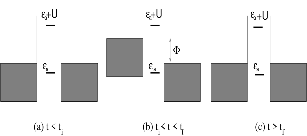
Figure 1: Energy level representation of interacting electrons in a quantum dot before, during, and after application of a bias pulse of amplitude $\Phi$ to the left lead, holding both the right lead chemical potential and the dot energy level, $\epsilon_{a}$, fixed. Here $U$ is the Coulomb interaction between electrons inside the dot.

Here $c_{a}^{{\dagger}\sigma}$ is an operator that creates an electron in the dot level $a$ with spin $\sigma$ and $c_{k\alpha}^{{\dagger}\sigma}$ creates an electron in a level $k$ in the $\alpha$-lead. Throughout the paper we adopt the following notation for the indices: Greek letters $\alpha$, $\beta$, $\gamma$ and $\delta$ label the left and right leads. Greek letter $\sigma$ labels the spin, and a sum over the $N$ spin components is implied whenever there is a pair of raised and lowered indices. Operator $n_{a}\equiv c_{a}^{{\dagger}\sigma}c_{a\sigma}$ counts the occupancy of level $a$ in the dot. Projection operators $\hat{P}_{1}$ and $\hat{P}_{2}$ can be written in terms of $n_{a}$ and project onto the single- and double-occupied dot, respectively. Parameters $\epsilon_{a}^{(1)}(t)$, $\epsilon_{a}^{(2)}(t)$, $V_{a;k}^{(1)}(t)$ and $V_{a;k}^{(2)}(t)$ are respectively the orbital energies and hybridization matrix elements for the quantum dot with one or two electrons. The projection operators enable the use of different couplings and orbital energies depending on the number of electrons in the dot. For simplicity, however, here we assume that the hybridization matrix elements are identical, and independent of level index and time: $V_{a;k\alpha}^{(1)}(t)=V_{a;k\alpha}^{(2)}(t)\equiv V$. We also assume that the electronic levels in the dot are the same (apart from the charging energy $U_{aa}$): $\epsilon^{(1)}_{a}(t)=\epsilon^{(2)}_{a}(t)=\epsilon_{a}(t)$. In Eq. 1, the original hybridization matrix elements are divided by a factor of $\sqrt{N}$ so that the dot level half-width due to the hybridization with either lead, $\Delta_{\alpha}=\pi\rho|V|^{2}=\Delta$, is independent of $N$, remaining finite in the $N\rightarrow\infty$ limit. The density of states per spin channel of either lead is denoted by $\rho$, here is taken to be constant. Coulomb interaction $U_{aa}$ is the repulsive energy between two electrons that occupy the same dot level $a$, while $U_{ab}$ is the interaction between electrons in different levels. Time-dependence may come in through the conducting leads, $\epsilon_{k\alpha}(t)=\epsilon_{k\alpha}+\Phi_{k\alpha}(t)$, the dot level, $\epsilon_{a}(t)=\epsilon_{a}+\Phi_{a}(t)$, or both. Functions $\Phi_{a}(t)$ and $\Phi_{k\alpha}(t)$ may have any time dependence. For instance Fig. 1 illustrates the case of a rectangular pulse bias potential applied to the left lead keeping both the dot level and right lead unchanged.

To permit a comparison of the dynamical $1/N$ approach to other methods we further simplify the above Hamiltonian. In the following we only consider the case of a single level, $a=0$, so for notational simplicity we define $U_{aa}\equiv U$ in the rest of the paper. The model then corresponds to the usual one considered by many other authors that treats only a single s-wave level in the quantum dot. However, we stress that the Hamiltonian, Eq. 1, can also be used to study more general and experimentally relevant models.

II.2 $1/N$ expansion of the wavefunction

The many-body wavefunction is constructed by systematically expanding the Hilbert space into sectors with increasing number of particle-hole pairs in the leads. Sectors with more and more particle-hole pairs are reduced by powers of $1/N$ in the expansion. The approach was originally introduced to study magnetic impurities in metalsVarma , mixed-valence compoundsGunnarsson and it was first applied to a dynamical atom-surface scattering problem by Brako and NewnsBrako . We have previously applied it to the scattering of alkaliErnie ; Onufriev and alkaline-earth ions such as calcium off metal surfacesMerino where in the latter case various Kondo effects may be expectedSNL ; Toulouse . The expansion of the time-dependent wavefunction for the lead-dot-lead system up to order O($1/N^{2}$) in the spin-singlet (more generally, SU(N)-singlet) sector may be written in terms of the scalar amplitudes $f(t)$, $b_{a;k\alpha}(t)$, $e_{L\gamma,k\alpha}(t)$, $d_{k\alpha,q\beta}(t)$, $s_{a;L\gamma,k\alpha,q\beta}(t)$, $a_{a;L\gamma,k\alpha,q\beta}(t)$, $g_{L\gamma,P\delta,k\alpha,q\beta}(t)$, and $h_{L\gamma,P\delta,k\alpha,q\beta}(t)$:

$$|\Psi(t)\rangle = f(t)~{}|0\rangle+\sum_{a;\ k,\alpha}b_{a;k\alpha}(t)~{}|a;k\alpha\rangle+\sum_{L,\ k,\gamma,\alpha}e_{L\gamma,k\alpha}(t)~{}|L\gamma,k\alpha\rangle+\sum_{q<k,\alpha,\beta}d_{k\alpha,q\beta}(t)~{}|k\alpha,q\beta\rangle$$ (2)

$$+ \sum_{a;\ L,\ q<k,\gamma,\alpha,\beta}s_{a;L\gamma,k\alpha,q\beta}(t)~{}{|a;L\gamma,k\alpha,q\beta\rangle}^{S}+\sum_{a;\ L,\ q<k,\gamma,\alpha,\beta}a_{a;L\gamma,k\alpha,q\beta}(t)~{}{|a;L\gamma,k\alpha,q\beta\rangle}^{A}$$

$$+ \sum_{L>P,\ q<k,\gamma,\delta,\alpha,\beta}g_{L\gamma,P\delta,k\alpha,q\beta}(t)~{}{|L\gamma,P\delta,k\alpha,q\beta\rangle}^{S}+\sum_{L>P,\ q<k,\gamma,\delta,\alpha,\beta}h_{L\gamma,P\delta,k\alpha,q\beta}(t)~{}{|L\gamma,P\delta,k\alpha,q\beta\rangle}^{A}$$

$$+ \{{\rm rest~{}of~{}Hilbert~{}space}\}\ .$$

The first line of this equation contains the O(1) amplitudes, the second line has the O($1/N$) terms, and the amplitudes in the third line are O($1/N^{2}$). Upper case Roman letters $L$ and $P$ label lead levels above the Fermi level, whereas lower case letters $k$ and $q$ label lead levels below the Fermi energy. Expressions for the basis states in the case of atoms scattered off metal surfaces can be found elsewhereOnufriev , but we rewrite them here for clarity. The vacuum state $|0\rangle$ represents an empty dot, with both leads filled with electrons up to the Fermi energy. The remaining states, which are all SU(N)-singlets due to the contracted spin indices $\sigma$ and $\sigma^{\prime}$, are:

$$|a;k\alpha\rangle = {{1}\over{\sqrt{N}}}~{}c^{\dagger\sigma}_{a}c_{k\alpha\sigma}|0\rangle$$

$$|L\gamma,k\alpha\rangle = {{1}\over{\sqrt{N}}}~{}c^{\dagger\sigma}_{L\gamma}c_{k\alpha\sigma}|0\rangle$$

$$|k\alpha,q\beta\rangle = {{1}\over{\sqrt{N(N-1)}}}~{}c^{\dagger\sigma}_{0}c_{k\alpha\sigma}c_{0}^{\dagger\sigma^{\prime}}c_{q\beta\sigma^{\prime}}|0\rangle$$

$${|a;L\gamma,k\alpha,q\beta\rangle}^{S} = {{1}\over{\sqrt{2N(N-1)}}}~{}\big{\{}c_{L\gamma}^{\dagger\sigma}c_{k\alpha\sigma}c^{\dagger\sigma^{\prime}}_{a}c_{q\beta\sigma^{\prime}}|0\rangle+c_{L\gamma}^{\dagger\sigma}c_{q\beta\sigma}c^{\dagger\sigma^{\prime}}_{a}c_{k\alpha\sigma^{\prime}}|0\rangle\big{\}}$$

$${|a;L\gamma,k\alpha,q\beta\rangle}^{A} = {{1}\over{\sqrt{2N(N+1)}}}~{}\big{\{}c_{L\gamma}^{\dagger\sigma}c_{k\alpha\sigma}c^{\dagger\sigma^{\prime}}_{a}c_{q\beta\sigma^{\prime}}|0\rangle-c_{L\gamma}^{\dagger\sigma}c_{q\beta\sigma}c^{\dagger\sigma^{\prime}}_{a}c_{k\alpha\sigma^{\prime}}|0\rangle\big{\}}$$

$${|L\gamma,P\delta,k\alpha,q\beta\rangle}^{S} = {{1}\over{\sqrt{2N(N-1)}}}~{}\big{\{}c_{L\gamma}^{\dagger\sigma}c_{k\alpha\sigma}c^{\dagger\sigma^{\prime}}_{P\delta}c_{q\beta\sigma^{\prime}}|0\rangle+c_{L\gamma}^{\dagger\sigma}c_{q\beta\sigma}c^{\dagger\sigma^{\prime}}_{P\delta}c_{k\alpha\sigma^{\prime}}|0\rangle\big{\}}$$

$${|L\gamma,P\delta,k\alpha,q\beta\rangle}^{A} = {{1}\over{\sqrt{2N(N+1)}}}~{}\big{\{}c_{L\gamma}^{\dagger\sigma}c_{k\alpha\sigma}c^{\dagger\sigma^{\prime}}_{P\delta}c_{q\beta\sigma^{\prime}}|0\rangle-c_{L\gamma}^{\dagger\sigma}c_{q\beta\sigma}c^{\dagger\sigma^{\prime}}_{P\delta}c_{k\alpha\sigma^{\prime}}|0\rangle\big{\}}.$$

We set the Fermi energy to zero ($\epsilon_{F}\equiv 0$) before the pulse is applied ($t<t_{i}$). An ordering convention is imposed on the above states such that $\epsilon_{q}<\epsilon_{k}<0$ and $\epsilon_{L}>\epsilon_{P}>0$. Fig. 2 shows a schematic representation of the different Hilbert space sectors appearing in the $1/N$ expansion up through $O(1/N^{2})$. Each row represents a different order in the $1/N$ expansion, increasing upon moving downwards in the diagram. The physical interpretation of each of the sectors is as follows: State $|L\gamma,k\alpha\rangle$ represents an electron excited to level $L$ in lead $\gamma$ along with a hole in level $k$ in lead $\alpha$. State $|k\alpha,q\beta\rangle$ represents configurations in which two electrons occupy the lowest level ($a=0$) of the quantum dot simultaneously, with two holes left behind in the leads. These configurations are suppressed in the limit $U\rightarrow\infty$. States ${|a;L\gamma,k\alpha,q\beta\rangle}^{S}$ and ${|a;L\gamma,k\alpha,q\beta\rangle}^{A}$ are symmetric (S) and antisymmetric (A) combinations of the configuration with one electron in level $L$ and holes in level $k$ of lead $\alpha$ and in level $q$ of lead $\beta$. The division of the sector into two parts reflects the fact that the state produced by an electron hopping to the dot from a continuum level $k$ while another electron is excited from $q$ to $L$ can be distinguished (because the electrons carry spin) from the state in which $k$ and $q$ are interchanged. A similar decomposition is carried out for the sectors with two particle-hole pairs described by amplitudes $g$ and $h$.

We neglect, at O($1/N^{2}$), the sector corresponding to a singly-occupied dot with a hole and two particle-hole pairs as the amplitude for this sector has 5 continuum indices. This sector is expected to be important for the physically interesting case of the Kondo and mixed-valent regimes with near single occupancy of the quantum dot. Its inclusion would presumably improve the behavior of the dynamical $1/N$ approach at long times, and we leave this for future work. Strictly speaking, through O($1/N^{2}$) we should also include sectors corresponding to a doubly-occupied quantum dot with one or two particle-hole pairs in addition to the two holes in the leads. However, as these configurations are described by amplitudes with up to 6 different continuum indices, and as the amplitudes for these sectors is small (due to the repulsive Coulomb interaction), the computational work required to include the amplitudes is excessive, and we drop them from the equations of motion.

The equations of motion for the amplitudes that appear in Eq. 2 are given in the Appendix. We note that the terms we keep in the $1/N$ expansion is equivalent to summing up Feynman diagrams, including the crossing ones, up to order $1/N^{2}$. The inclusion of crossing diagrams is significant because it is these diagrams that are known to be responsible for the recovery of Fermi liquid behavior at low temperaturesBickers , and the disappearance of the Kondo effect in the spinless $N\rightarrow 1$ limit.

II.3 Calculation of observable quantities

We conclude our discussion of the dynamical $1/N$ method by explaining how observable quantities such as the currents are calculated. At zero temperatures, the initial state of the system prior to application of the bias is chosen to be the ground state, which is obtained by the power method. Integrating the equations of motion forward in time then yields $|\Psi(t)\rangle$, and expectation values of observables, $\hat{O}$, are calculated periodically during the course of the time evolution:

$$\langle\hat{O}(t)\rangle=\langle\Psi(t)|\hat{O}|\Psi(t)\rangle\ .$$ (4)

For the particulars of how to calculate the expectation value of the current operators, see the Appendix.

Most of the results presented in the paper, with the exception of those shown in the final figure, are for the case of zero temperature. At non-zero temperatures we must extend the methodMerino . Suppose that at an initial time $t=0$, prior to application of the bias, we could find the complete set of energy eigenstates and values $\{|\Psi_{n}(0)\rangle,~{}E_{n}\}$ satisfying $H|\Psi_{n}(0)\rangle=E_{n}|\Psi_{n}(0)\rangle$. Each of these eigenstates could then be evolved forward in time yielding $\{|\Psi_{n}(t)\rangle\}$. The combined thermal and quantum average of any observable quantity, $\hat{O}$, would then be given at time $t$ by:

$$\langle\hat{O}(t)\rangle={{1}\over{Z}}\sum_{n}\langle\Psi_{n}(t)|\hat{O}|\Psi_{n}(t)\rangle\exp\bigg{\{}-{{E_{n}}\over{k_{B}T}}\bigg{\}}$$ (5)

where

$$Z=\sum_{n}\exp\bigg{\{}-{{E_{n}}\over{k_{B}T}}\bigg{\}}$$ (6)

is as usual the partition function of the system. However, as the Hilbert space is enormous in size, the determination of the whole set of time-evolved many-body wavefunctions is prohibitively difficult. Instead we sample the Hilbert space by creating a finite, random, set of wavefunctions: $\{|\Xi_{n}\rangle,~{}n=1,\ldots,n_{sample}\}$. The wavefunctions are generated by assigning random numbers to the amplitudes that describe the different sectors of the wavefunction, Eq. 2. Each of these randomly generated wavefunctions is then weighted by half of the usual Boltzmann factor,

$$|\tilde{\Psi}_{n}(0)\rangle=\exp\bigg{\{}-{{H(0)}\over{2k_{B}T}}\bigg{\}}|\Xi_{n}\rangle\ ,$$ (7)

and the resulting set of weighted wavefunctions is time-evolved to yield $\{|\tilde{\Psi}_{n}(t)\rangle\}$. (The wavefunctions are weighted by half the usual Boltzmann factor so that thermal expectation values, which depend on the square of the wavefunctions, have the correct weight.) Thermal averages of each observable such as the current are calculated periodically during the course of the integration forward in time:

$$\langle\hat{O}(t)\rangle={{1}\over{Z}}\sum_{n=1}^{n_{sample}}\langle\tilde{\Psi}_{n}(t)|\hat{O}|\tilde{\Psi}_{n}(t)\rangle$$ (8)

where

$$Z=\sum_{n=1}^{n_{sample}}\langle\tilde{\Psi}_{n}(t)|\tilde{\Psi}_{n}(t)\rangle=\sum_{n=1}^{n_{sample}}\langle\tilde{\Psi}_{n}(0)|\tilde{\Psi}_{n}(0)\rangle\ .$$ (9)

At the very lowest temperatures only a single sample is needed as the approach then reduces to the zero-temperature power method described above. At non-zero but moderate temperatures, thermal averages over $n_{sample}=30$ random wavefunctions suffice, and the convergence of the thermal average may be easily checked by increasing the number of samples. We stress that time dependence comes in only via the wavefunctions. This makes the present approach rather straightforward, avoiding cumbersome Green’s function formalisms based on the Keldysh or Kadanoff-Baym techniques. On the other hand, the approach is not useful at very high temperatures as an excessive number of samples is then required.

We now present an intuitive picture of how electronic transitions take place as the current flows through the quantum dot. Fig. 2 shows some of the sectors, up to O(1/$N^{2}$), that contribute to the current through a dot subject to the rectangular pulse bias shown in Fig. 1. When the bias is switched on, electronic transitions between the dot and the leads take place. Sectors shown in Fig. 2 in which an electron travels from the left to the right leads creating cross-lead particle-hole excitations make the most important contribution to the current. The current through the dot is a consequence of the formation of particle-hole pairs, with holes accumulating in one lead and particles in the other. Sectors of the Hilbert space with increasing numbers of particle-hole pairs, and hence higher order in $1/N$, become populated as time goes on. Electronic transitions back down to lower order sectors also occur, of course, since the Hamiltonian is Hermitian. However, because the phase space of sectors with increasing numbers of particle-hole pairs grows rapidly with the number of pairs, when the system is driven out-of-equilibrium, reverse processes back down to lower orders occur less frequently. This irreversibility may be quantified in terms of an increasing entropyOnufriev .

III Response to a small, symmetric, step in the bias potential

We first apply the dynamical $1/N$ approach to study the response of a quantum dot to a small, symmetric, step bias potential. We use parameters appropriate for a semiconducting quantum dot. We either take $U\rightarrow\infty$ or, more realistically, set $U=1$ or $2$ meV comparable to the values reported by Goldhaber-Gordon et al. for the single electron transistor built on the surface of a GaAs/AlGaAs heterostructure that led to the reported Kondo effectGoldhaber ; Gores . We further set the dot-lead half-width to be $\Delta=0.4$ meV, and $\epsilon_{a}=-2\Delta$. Thus in the case of spinning electrons the dot is in the Kondo regime. In a real SET there are several quantized levels with a typical spacing of order $0.4$ meV. However, as mentioned in the previous section, here for simplicity we consider only the case of a single energy level in the dot. At time $t_{i}=0.5\hbar/\Delta$ the bias on the left lead is suddenly turned on, raising the Fermi energy by $\Phi/2$, while the right lead is shifted down by the opposite amount, -$\Phi/2$, and the dot level is held fixed. The size of the bias is chosen to be $\Phi=0.05\Delta$ which is small enough to induce a linear response in the current.

The leads are assumed to be described by a flat band of constant density of states with all energies taken to be relative to the Fermi energy. The band is taken to be symmetrical about the Fermi energy with a half-bandwidth set at $D=4$ meV. We use $M=30$ discrete levels both above, and below, the Fermi energy in our calculations, except for the O($1/N^{2}$) amplitudes $g_{L\gamma,P\delta,k\alpha,q\beta}(t)$ and $h_{L\gamma,P\delta,k\alpha,q\beta}(t)$. As these amplitudes each have four continuum indices, we retain only 10 levels above, and below, the Fermi energy. This turns out to suffice as there is little change when only 5 levels are retained. To improve the discrete description, the continuum of electronic states in the conducting leads is sampled unevenly: the mesh is made finer near the Fermi energy to account for particle-hole excitations of low energy. Specifically, the discrete energy levels below the Fermi energy are of the following form:

$$\epsilon_{k}=-{{D}\over{e^{\gamma}-1}}~{}[e^{\gamma(k-1/2)/M}-1],\ \ \ k=1,2,\cdots,M\$$ (10)

with a similar equation for levels above the Fermi energy. Thus, the spacing of the energy levels close to the Fermi energy is reduced from the evenly spaced energy interval of $D/M$ by a factor of $\gamma/(e^{\gamma}-1)\approx 1/13$ for a typical choice of the sampling parameter $\gamma=4$. The matrix elements $V^{(i)}_{a;k\alpha}$ are likewise adjusted to compensate for the uneven sampling of the conducting levelsMerino . We note that the discretization of the continuum of electronic states in the leads means that we can only study pulses of duration less than a cutoff time: $t_{cutoff}\approx 2\pi\hbar/\delta$, where $\delta\approx D/(13M)$ is the level spacing close to the Fermi energy of the conducting leads. As we show below, however, the $1/N$ expansion itself imposes a more severe restriction on the reliability of the method at long times.

III.1 Noninteracting spinless electrons ($N=1$)

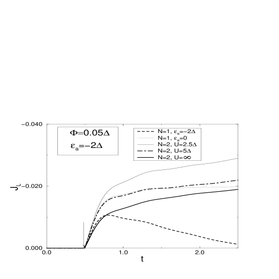
Figure 3: Response of the electric current per spin channel between the left lead and a quantum dot to a small symmetric bias step potential. Time is given in units of $\hbar/\Delta$ where $\Delta=0.4$ meV, and current is in units of $e/h$. A small, symmetric, step bias potential of amplitude $\Phi/2=0.025\Delta$ is applied to the left lead and an opposing bias of $-0.025\Delta$ is applied to the right lead. The arrow at time $t=t_{i}=0.5\hbar/\Delta$ indicates the moment when the step in the bias is turned on. The electronic level in the dot is held fixed at energy $\epsilon_{a}=-2\Delta$. (For comparison in the $N=1$ case we also show results for $\epsilon_{a}=0$.) The non-interacting spinless case as calculated within the dynamical $1/N$ approximation upon setting $N=1$ is compared to the case of interacting electrons ($N=2$) with $U=1$ and $2$ meV and $U=\infty$. Currents initially grow and then decay (evident in the time range shown here only for the case $N=1$ and $\epsilon_{a}=-2\Delta$) despite the fact that the bias remains on. The eventual decay of the currents is a consequence of continued production of particle-hole pairs, saturating the high-order sectors of the $1/N$ expansion. The response current is strongly enhanced in the interacting case with respect to the spinless case due to the presence of a Kondo resonance at the Fermi level of the leads. For $U=1$ and $2$ meV, the current is further enhanced reflecting an increase in the Kondo temperature.

The case of spinless electrons deserves special attention as it provides a stringent test of the $1/N$ expansion, and is also exactly solvable. For an Anderson impurity model at equilibrium it is knownGunnarsson that the occupancy of the impurity at $N=1$ is accurate to within 1% of the exact result when terms in the wavefunction expansion are kept up through order $1/N^{2}$. In the dynamical case shown in Fig. 3, however, we find that for $\epsilon_{a}=-2\Delta$ the currents decay in time despite the fact that the bias remains turned on. Insight into the breakdown of the dynamical $1/N$ expansion can be gleaned from the equilibrium problem as discussed by Gunnarssson and SchönhammerGunnarsson . They observe that the parameter range $\epsilon_{a}\ll-\Delta$ is an unfavorable one for the $1/N$ expansion. The O($1$) approximation in this limit differs qualitatively from the O($1/N$) and O($1/N^{2}$) approximations. In particular there is a large change in variational ground state energy (97% in the case of $\epsilon_{a}=-\Delta$) going from the O($1$) to O($1/N$) approximations. This compares to a change of only 18% in energy for the $\epsilon_{a}=0$ case. In the dynamical problem the observation likewise suggests that the case $\epsilon_{a}=-2\Delta$ depicted in Fig. 3 is also unfavorable for the $1/N$ expansion as higher order sectors may be expected to contribute substantially to the wavefunction. By contrast the other $N=1$ case of $\epsilon_{a}=0$ shown in Fig. 3 exhibits a clear plateau in the currents. We interpret this behavior as follows: As the dot energy level is raised from $\epsilon_{a}=-2\Delta$ to $0$, the many-body wavefunction moves closer to the beginning “root” state of the Hilbert space expansion, the state $|0\rangle$ in Fig. 2 for which the dot level is empty. Higher-order terms in the $1/N$ expansion are less important in this limit, and the expansion is more accurate.

The limited number of particle-hole pairs retained in the $1/N$ expansion means that electron transfer from one lead to the other ceases when the higher order sectors become significantly populated. Therefore, we conclude that the dynamical $1/N$ approach is limited to rather short times after the step in the bias is applied. Inclusion of higher-order sectors in the $1/N$ expansion would presumably permit accurate time-evolution for longer times. The amplitude of the $O(1/N^{2})$ sector for the case of Fig. 3 is quite small when the current starts to decay, consistent with the observation that the amplitude of the empty dot sectors (first column in Fig. 2) are small in comparison to the singly-occupied sectors (second column of Fig. 2), in the the Kondo and mixed-valence regimes. Including the O($1/N^{2}$) sector consisting of two particle-holes in the leads, an electron in the dot and an extra hole in the leads should improve the behavior of the current at longer times. However as a practical matter the rapid growth in computational complexity at high orders in the $1/N$ expansion prohibits extensions to arbitrarily high order. Cluster expansions based upon exponentials of particle-hole creation operatorsSebastian may offer a way to obtain more satisfactory behavior at long times.

III.2 Interacting spinning electrons ($N=2$)

Physical electrons have spin, and since $N=2$ is a more favorable case from the standpoint of the $1/N$ expansion, we expect (and find) improved behavior. The Coulomb repulsion $U$ reduces the size of higher-order corrections as it acts in part to suppress charge-transfer through the dot that leads to the formation of the particle-hole pairs. Furthermore the Kondo effect in the limit $\epsilon_{a}\ll-\Delta$ is recovered already at O($1$) in the $1/N$ expansion. As shown in Fig. 3, for $U\rightarrow\infty$ there is a strong enhancement in the current in comparison to the spinless case ($N=1$). This is as expected from the increase of spectral weight at the Fermi level of the leads due to the Kondo resonance. The current is further enhanced at finite $U=1$ meV. This can be understood from $1/N$ calculations of the spectral density at equilibrium. A decrease in $U$ results in an increase in the spectral weight at the Fermi energy, reflecting a corresponding increase in the Kondo energy scale (see Fig. 9 of Ref. Gunnarsson, ). The point is also illustrated by an analytical estimate of the Kondo temperature for finite $U$ based on weak-coupling renormalization-group scalingHaldane :

$$k_{B}T_{K}\approx\sqrt{{{\Delta_{dot}U}\over{2}}}~{}\exp{\bigg{\{}{{\pi\epsilon_{a}(\epsilon_{a}+U)}\over{\Delta_{dot}U}}}\bigg{\}}\ .$$ (11)

Here $\Delta_{dot}=\Delta_{L}+\Delta_{R}=2\Delta$ is the half-width of the dot level due to its hybridization with both leads. This formula yields $T_{K}\approx 4$K. As the weak-coupling expression Eq. 11 is only reliable at small values of $U$, it likely overestimates the Kondo temperature in the present case of $U/\Delta=2.5$. It is worth comparing the Kondo temperature so obtained with the value extracted from the $U\rightarrow\infty$ Bethe-ansatz expressionHewson ,

$$k_{B}T_{K}=D{{e^{1+C-{{3}\over{2N}}}}\over{2\pi}}\bigg{(}{\Delta_{dot}\over{\pi D}}\bigg{)}^{1/N}\exp{\bigg{\{}{{\pi\epsilon_{a}}\over{\Delta_{dot}}}}\bigg{\}}\ ,$$ (12)

where $C=0.577216$ is Euler’s constant. Taking $N=2$, Eq. 12 gives only $T_{K}\approx 185$ mK.

Hence, the increase in the Kondo temperature obtained from Eqs. 12 and 11 as $U$ is decreased from infinite to finite values is consistent with the enhancement of the current shown in Fig. 3. We use Eq. 11 to estimate the Kondo temperature at finite-$U$ in the following section.

IV Response to a large rectangular pulse bias potential

In this section we study the response of the quantum lead-dot-lead system to a large rectangular pulse bias potential, driving the system well beyond the linear response regime. As the response of the dot-lead system is highly non-linear, this situation is quite instructive. We again study both the $N=1$ and $N=2$ cases, and use the same values for $\epsilon_{a}$ and $U$ as in the previous section but with $\Delta=0.2$ meV. The rectangular pulse bias potential is applied as follows. At time $t_{i}=0.5\hbar/\Delta$, a sudden upward shift of the bias with amplitude $\Phi$ is applied to the left lead, leaving the dot energy level unchanged, and the right lead unbiased as depicted in Fig. 1. At a later time $t=t_{f}$ the bias is turned off.

IV.1 Noninteracting spinless electrons ($N=1$)

The abrupt rise in the bias generates a ringing in the response currents as a result of coherent electronic transitions between electrons at the Fermi energy in the leads and the dot level. The period of these oscillations was predicted to beWingreenb :

$$t_{p}={2\pi\hbar\over|\Phi-\epsilon_{a}|}.$$ (13)

Fig. 4 shows, for the case $\epsilon_{a}=-2\Delta$, the response current between the left lead and the dot upon setting $N=1$ in the $1/N$ expansion. The oscillation period accords with Eq. 13. For the sake of comparison, Fig. 4 also shows the current for the case of interacting, spinning, electrons. Note that oscillation period changes when interactions are turned on. As discussed in the next subsection, this is a consequence of the formation of Kondo resonances at the Fermi energy in each lead. It is remarkable that the $1/N$ approach reproduces, in the $N=1$ limit, the period of the oscillations expected from Eq. 13. Unlike NCA, the $1/N$ approach recovers the expected features of non-interacting electrons in the $N=1$ limit. In particular, many-body Kondo resonances disappearGunnarsson at $N=1$ as they must. As mentioned above, the recovery of independent-particle physics can be attributed to the presence of crossing diagrams in the $1/N$ expansion.

Also of interest is the duration of the initial response peak. The transient response time is shorter in the case of noninteracting spinless electrons. The transient response fades away more slowly because the repulsive Coulomb interaction inhibits electron motion through the dot.

IV.2 Interacting spinning electrons ($N=2$)

In equilibrium it is well known that a Kondo resonance can form at the Fermi energy of the leads. For the steady state case of constant bias potential, previous NCA calculations of spectral density predicted the splitting of the Kondo peakWingreen into two resonances, one at the Fermi energy of each lead. The situation studied here is different as we analyze the response to a short pulse rather than the steady state behavior. Nevertheless, the behavior is still consistent with the split Kondo peak picture.

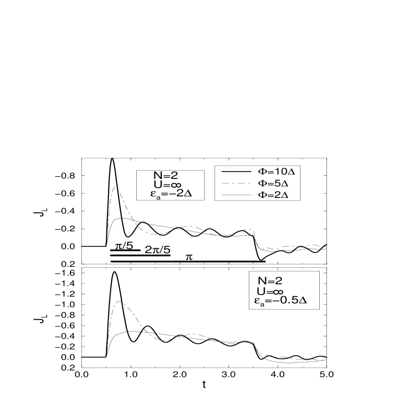
Figure 5: Dependence of the electronic current per spin channel between the left lead and the quantum dot on the amplitude, $\Phi$, of the externally applied rectangular pulse bias potential (see Fig. 1). Time is in units of $\hbar/\Delta$ where $\Delta=0.2$ meV, and current is in units of $e/h$. We consider interacting spinning electrons ($N=2$) and take $U\rightarrow\infty$. The quantum dot level is either in the Kondo regime ($\epsilon_{a}/\Delta=-2$) or in the mixed valent regime ($\epsilon_{a}/\Delta=-0.5$). The pulse starts at time $t=0.5\hbar/\Delta$ and ends at time $t=3.5\hbar/\Delta$. The current is plotted for different applied biases: $\Phi=2\Delta,5\Delta,$ and $10\Delta$. A comparison of time scales (horizontal lines) shows that the period of the oscillations does not obey Eq. 13 but rather $t_{p}=2\pi\hbar/\Phi$.

Fig. 5 shows that the response current does not obey Eq. 13. Instead the current oscillates with a period that is independent of $\epsilon_{a}$, and depends only on the bias. The period can be seen to be $2\pi\hbar/\Phi$, which agrees with Eq. 13 only upon setting $\epsilon_{a}=0$. Fig. 6 also demonstrates that the period of the oscillations remains nearly constant as the energy of the quantum dot level is varied from $\epsilon_{a}=0$ (mixed-valence regime) to $\epsilon_{a}=-3\Delta$ (Kondo regime). Large biases split the Kondo peak in two, and the resulting many-body resonances are separated by energy $\Phi$. Electronic transitions between these two peaks induce oscillations of period $2\pi\hbar/\Phi$. The $1/N$ calculation agrees qualitatively with the NCA calculation of Plihal, Langreth, and NordlanderPlihal . Figs. 5 and 6 show that the split-peak interpretation holds even for very large biases, $\Phi=2\Delta$ to $10\Delta$, and also in the mixed-valence regime. Fig. 6 also shows that the magnitude of the response current gradually decreases, and the transient oscillations damp out more quickly, as the dot energy level is moved downwards in energy. Insight into this behavior may again be attained from study of a quantum dot in equilibrium. In the limit $\epsilon_{a}/\Delta\rightarrow-\infty$ the Kondo scale vanishes and the spectral weight at the Fermi energy is suppressed. The dot enters the Coulomb blockade regime, inhibiting the flow of current.

Finally we discuss the effect of non-zero temperature on the response currents. Fig. 7 shows, for both noninteracting spinless and interacting spinning electrons, the currents at three temperatures: $T=100$ mK, $T=300$ mK and $500$ mK. The latter temperature is sufficiently high that multiple particle-hole pairs will be excited, as the level spacing is only $D/(13M)\approx 120$ mK at the Fermi energy; therefore the Hilbert space restriction to at most two particle-hole pairs is a severe limitation. Nevertheless, there is little change in the response of the spinless electrons as the temperature is increased. This is as it should be since the temperatures are still well below the Fermi temperature of the leads. By contrast the $N=2$ case shows a significant decrease in the current magnitude, and especially the oscillations, at the higher temperatures. Using the finite-$U$ formula Eq. 11 with $U/\Delta=10$, yields $T_{K}\approx 600$ mK. Considering the uncertainities involved in estimating the Kondo temperature (Eq. 11 gives the order of magnitude but the exact multiplicative factor is unknown) we can expect a suppression of the Kondo resonance and its associated effects at $500$ mK. The behavior of the currents shown in Fig. 7 is consistent with this interpretation, as the period of the transient oscillations decreases to approach that of the spinless system.

V Conclusions

We have presented a method for calculating the response of a quantum dot to time-dependent bias potentials. The approach, which is based upon a truncation of the Hilbert space, is systematic because corrections can be incorporated by including higher powers in the $1/N$ expansion. In agreement with previous approaches we find coherent oscillations in the response currents at low temperatures. We note that although the frequency of these oscillations is of order a terahertz for parameters typical of quantum dot devices, it should be possible to detect the oscillations experimentallyNakamura . The dynamical $1/N$ approach permits a realistic description of the quantum dot as finite Coulomb repulsion and multiple dot levels may be modeled. For typical device parameters, response currents are qualitatively similar to those found in the $U\rightarrow\infty$ limit. However, the magnitude of the current is larger.

We also discussed an extension of the dynamical $1/N$ expansion to treat the case of non-zero temperature. In the case of interacting spinning electrons the magnitude of the currents, and the nature of the transient response are sensitive to relative size of the system temperature in comparison to the Kondo temperature. In contrast non-interacting spinless electrons show little temperature dependence.

The dynamical $1/N$ approach complements other methods such as NCA and the TDMRG algorithm. The primary limitation of the dynamical $1/N$ approach comes from the truncation of the Hilbert space in which only a small number of particle-hole pairs (in this paper, at most two) are permitted. Hence, as it stands the method is not well suited for the study of steady state situations, and we cannot use it, for instance, to answer the question of whether or not a lead-dot-lead system exhibits coherent oscillations at long timesColeman ; Rosch . As NCA sums up an infinite set of Feynman diagrams, including ones with arbitrary numbers of particle-hole pairs, it provides a far better description of long-time behavior, including steady state current flow. For the same reason NCA is also superior at high temperature. However finite Coulomb interactions and other realistic features of lead-dot-lead systems are technically difficult to incorporate within NCA, but not in the dynamical $1/N$ method. Also, NCA shows unphysical behavior in the mixed valence regime, at very low temperatures, and in the spinless $N=1$ limit. The dynamical $1/N$ approach does not suffer from these pathologies. The method shares some features with the TDMRG algorithm as both are real-time approaches that truncate the Hilbert space in a systematic, though in a different, fashion. Unlike the present approach, TDMRG can treat strong electron interactions between electrons in the leads and can be used to study tunneling between Luttinger liquidsCazalilla . On the other hand, non-interacting electrons in the leads are treated exactly within the dynamical $1/N$ approach. In TDMRG these require as much or more computational effort as interacting electrons.

A complete description of the electronic transport properties in a SET would require taking into account the whole energy spectrum of the quantum dot and would include both the direct Coulomb repulsion and spin-exchange between electrons in different energy levels of the dot. Also the conducting leads should be described by realistic densities of states. The dynamical $1/N$ approach is well suited to accommodate these complications. Another aspect worth further attention is the case of orbital degeneracy of the dot levels. As the degeneracy increases, the Kondo resonance strengthens, and its width decreasesKroha . A combined experimental and theoretical exploration of the effect of orbital degeneracy on transport properties would be interesting. Finally, it should also be possible to extend the method to describe two coupled quantum dots attached to leadsAguado . Competition between Kondo resonances and spin-exchange between the two dots leads to unusual features such as a non-Fermi liquid fixed pointJones ; Affleck . Probing nonlinear transport as the parameters are tuned through this fixed pointGeorges could possibly shed some light on the physics of heavy-fermions materials.

VI Appendix

In this Appendix we present details of the equations of motion and the calculation of the currents.

VI.1 Equations of Motion

Equations of motion appropriate for the atom-surface scattering problem have been published elsewhereOnufriev . We rewrite them here, generalizing the equations to include two sectors that are of order O($1/N^{2}$) and substituting two conducting leads for the metallic surface. To remove diagonal terms in the equations of motion we introduce the phase factor

$$\phi^{(i)}_{a}(t)\equiv{{1}\over{\hbar}}~{}\int^{t}_{0}\epsilon^{(i)}_{a}(t^{\prime})dt^{\prime}\ ,$$ (14)

which is the phase of the quantum dot level when it is decoupled from the leads, and

$$\phi_{k\alpha}(t)\equiv{{1}\over{\hbar}}~{}\int^{t}_{0}\epsilon_{k\alpha}(t^{\prime})dt^{\prime}\ ,$$ (15)

the phase of the electronic levels in the decoupled leads. Upon projecting the time-dependent Schrödinger equation onto the different sectors of the Hilbert space, the equations of motion may then be extracted. Following Refs. Ernie, and Onufriev, we use capital letters to denote amplitudes in which the diagonal phases of the corresponding lower case amplitudes have been factored out:

$$i\hbar{d\over{dt}}F = \sum_{a;k\alpha}V^{(1)*}_{a;k\alpha}\exp\{i[\phi_{k\alpha}(t)-\phi^{(1)}_{a}(t)]\}\ B_{a;k\alpha}$$

$$i\hbar{d\over{dt}}B_{a;k\alpha} = V^{(1)}_{a;k\alpha}\ \exp\{i[\phi^{(1)}_{a}(t)-\phi_{k\alpha}(t)]\}\ F$$

$$+ \delta_{a,0}~{}\sqrt{1-1/N}\sum_{q,\beta}V^{(2)*}_{0;q\beta}\exp\{-i[U-\phi_{q\beta}(t)+2\phi^{(2)}_{0}(t)-\phi^{(1)}_{0}(t)]\}\ [\theta(k-q)~{}D_{k\alpha,q\beta}+\theta(q-k)~{}D_{q\beta,k\alpha}]$$

$$+ {{1}\over{\sqrt{N}}}\sum_{L\gamma}V^{(1)}_{a;L\gamma}\ \exp\{i[\phi^{(1)}_{a}(t)-\phi_{L\gamma}(t)]\}\ E_{L\gamma,k\alpha}$$

$$i\hbar{d\over{dt}}E_{L\gamma k\alpha} = {{1}\over{\sqrt{N}}}\sum_{a}V^{(1)*}_{a;L\gamma}\ \exp\{i[\phi_{L\gamma}(t)-\phi^{(1)}_{a}(t)]\}\ B_{a;k\alpha}$$

$$+ \sqrt{{{N-1}\over{2N}}}\sum_{a;q\beta}V^{(1)*}_{a;q\beta}\exp\{i[\phi_{q\beta}(t)-\phi^{(1)}_{a}(t)]\}[\theta(k-q)\ S_{a;L\gamma,k\alpha,q\beta}+\theta(q-k)\ S_{a;L\gamma,q\beta,k\alpha}]$$

$$+ \sqrt{{{N+1}\over{2N}}}\sum_{a;q\beta}V^{(1)*}_{a;q\beta}\exp\{i[\phi_{q\beta}(t)-\phi^{(1)}_{a}(t)]\}[\theta(k-q)\ A_{a;L\gamma,k\alpha,q\beta}-\theta(q-k)\ A_{a;L\gamma,q\beta,k\alpha}]$$

$$i\hbar{d\over{dt}}D_{k\alpha,q\beta} = \sqrt{1-1/N}\ V^{(2)}_{0;q\beta}\ \exp\{i[U-\phi_{q\beta}(t)+2\phi^{(2)}_{0}(t)-\phi^{(1)}_{0}(t)]\}\ B_{0;k\alpha}$$

$$+ \sqrt{1-1/N}~{}V^{(2)}_{0;k\alpha}~{}\exp\{i[U-\phi_{k\alpha}(t)+2\phi^{(2)}_{0}(t)-\phi^{(1)}_{0}(t)]\}~{}B_{0;q\beta}$$

$$+ \sqrt{{{2}\over{N}}}\sum_{L\gamma}V^{(2)}_{0;L\gamma}\ \exp\{i[U-\phi_{L\gamma}(t)+2\phi^{(2)}_{0}(t)-\phi^{(1)}_{0}(t)]\}~{}S_{0;L\gamma,k\alpha,q\beta}$$

$$i\hbar{d\over{dt}}S_{a;L\gamma,k\alpha,q\beta} = \delta_{a,0}\ \sqrt{{{2}\over{N}}}\ V^{(2)*}_{0;L\gamma}\ \exp\{-i[U-\phi_{L\gamma}+2\phi^{(2)}_{0}(t)-\phi^{(1)}_{0}(t)]\}D_{k\alpha,q\beta}$$

$$+ \sqrt{{{N-1}\over{2N}}}~{}[V^{(1)}_{a;q\beta}\exp\{i[\phi^{(1)}_{a}(t)-\phi_{q\beta}(t)]\}\ E_{L\gamma,k\alpha}+V^{(1)}_{a;k\alpha}\exp\{i[\phi^{(1)}_{a}(t)-\phi_{k\alpha}(t)]\}\ E_{L\gamma,q\beta}]\$$

$$+ {{1}\over{\sqrt{N}}}\sum_{J\delta}V^{(1)*}_{a;J\delta}\exp\{i[\phi_{J\delta}(t)-\phi^{(1)}_{a}(t)]\}[\theta(L-J)G_{a;L\gamma,J\delta,k\alpha,q\beta}+\theta(J-L)G_{a;J\delta,L\gamma,k\alpha,q\beta}]$$

$$i\hbar{d\over{dt}}A_{a;L\gamma,k\alpha,q\beta} = \sqrt{{{N+1}\over{2N}}}~{}[V^{(1)}_{a;q\beta}\exp\{i[\phi^{(1)}_{a}(t)-\phi_{q\beta}(t)]\}\ E_{L\gamma,k\alpha}-V^{(1)}_{a;k\alpha}\exp\{i[\phi^{(1)}_{a}(t)-\phi_{k\alpha}(t)]\}\ E_{L\gamma,q\beta}]\$$

$$+ {{1}\over{\sqrt{N}}}\sum_{J\delta}V^{(1)*}_{a;J\delta}\exp\{i[\phi_{J\delta}(t)-\phi^{(1)}_{a}(t)]\}[\theta(L-J)H_{a;L\gamma,J\delta,k\alpha,q\beta}-\theta(J-L)H_{a;J\delta,L\gamma,k\alpha,q\beta}]$$

$$i\hbar{d\over{dt}}G_{L\gamma,J\delta,k\alpha,q\beta} = {{1}\over{\sqrt{N}}}V^{(1)*}_{a;J\delta}\exp\{i[\phi_{J\delta}(t)-\phi^{(1)}_{a}(t)]\}S_{a;L\gamma,k\alpha,q\beta}+{{1}\over{\sqrt{N}}}V^{(1)*}_{a;L\gamma}\exp\{i[\phi_{L\gamma}(t)-\phi^{(1)}_{a}(t)]\}S_{a;J\delta,k\alpha,q\beta}$$

$$i\hbar{d\over{dt}}H_{L\gamma,J\delta,k\alpha,q\beta} = {{1}\over{\sqrt{N}}}V^{(1)*}_{a;J\delta}\exp\{i[\phi_{J\delta}(t)-\phi^{(1)}_{a}(t)]\}A_{a;L\gamma,k\alpha,q\beta}-{{1}\over{\sqrt{N}}}V^{(1)*}_{a;L\gamma}\exp\{i[\phi_{L\gamma}(t)-\phi^{(1)}_{a}(t)]\}A_{a;J\delta,k\alpha,q\beta}\ .$$ (16)

Here $\theta(k-q)$ and similar terms are unit step functions that enforces the ordering convention on the continuum indices. The equations of motion are numerically integrated forward in time using a fourth-order Runge-Kutta algorithm with adaptive time steps. We monitor the normalization of the wavefunction to ensure that any departure from unitary evolution remains small, less than $10^{-6}$.

VI.2 Calculation of Currents

A consideration of the rate of change of the quantum dot occupancy, as determined from the commutator $[n_{a},~{}H]$, permits the straightforward identification of the current operators between the dot and the left and right leads:

$$J_{\alpha} = {{e}\over{\hbar\sqrt{N}}}\sum_{a;k}\bigg{\{}i[V^{(1)*}_{a;k\alpha}\hat{P}_{1}+V^{(2)*}_{a;k\alpha}\hat{P}_{2}]c_{k\alpha}^{{\dagger}\sigma}c_{a\sigma}+H.c\bigg{\}}$$ (17)

$$= -{{2e}\over{\hbar\sqrt{N}}}{\rm Im}\bigg{\{}\sum_{a;k}[V^{(1)*}_{a;k\alpha}\hat{P}_{1}+V^{(2)*}_{a;k\alpha}\hat{P}_{2}]c_{k\alpha}^{{\dagger}\sigma}c_{a\sigma}\bigg{\}}$$

where as before the Greek index $\alpha$ refers to either the left or right lead. The expectation value of the current is calculated as the quantum and thermal average of the operator Eq. 17. For each time-evolved wavefunctions, $\tilde{\Psi}_{n}(t)$, the corresponding expected current may be expressed in terms of the amplitudes in the different sectors:

$$\langle\tilde{\Psi}_{n}(t)|J_{\alpha}|\tilde{\Psi}_{n}(t)\rangle=-{{2e}\over{\hbar}}~{}{\rm Im}\bigg{\{}\sum_{a;k}V^{(1)*}_{a;k\alpha}\exp\{i[\phi_{k\alpha}(t)-\phi^{(1)}_{a}(t)]\}F^{*}B_{a;k\alpha}$$ (18)

$$+ \sqrt{1-1/N}\sum_{k,q\beta}V^{(2)*}_{0;k\alpha}\exp\{-i[Ut-\phi_{k\alpha}(t)+2\phi^{(2)}_{0}(t)-\phi^{(1)}_{0}(t)]\}B^{*}_{0;q\beta}[\theta(k-q)D_{k\alpha,q\beta}+\theta(q-k)D_{q\beta,k\alpha}]$$

$$+ {{1}\over{\sqrt{N}}}\sum_{a;L,q\beta}V^{(1)*}_{a;L\alpha}\exp\{i[\phi_{L\alpha}(t)-\phi^{(1)}_{a}(t)]\}E^{*}_{L\alpha;q\beta}B_{a;q\beta}$$

$$+ \sqrt{{{N-1}\over{2N}}}\sum_{a;q,L\gamma,k\beta}V^{(1)*}_{a;q\alpha}\exp\{i[\phi_{q\alpha}(t)-\phi^{(1)}_{a}(t)]\}E^{*}_{L\gamma,k\beta}[\theta(k-q)S_{a;L\gamma,k\beta,q\alpha}+\theta(q-k)S_{a;L\gamma,q\alpha,k\beta}]$$

$$+ \sqrt{{{N+1}\over{2N}}}\sum_{a;q,L\gamma,k\beta}V^{(1)*}_{a;q\alpha}\exp\{i[\phi_{q\alpha}(t)-\phi^{(1)}_{a}(t)]\}E^{*}_{L\gamma,q\alpha}[\theta(k-q)A_{a;L\gamma,k\beta,q\alpha}-\theta(q-k)A_{a;L\gamma,q\alpha,k\beta}]$$

$$+ \sqrt{{{2}\over{N}}}\sum_{L,k\gamma,q\beta}V^{(2)*}_{0;L\alpha}\exp\{-i[Ut-\phi_{k\gamma}(t)+2\phi^{(2)}_{0}(t)-\phi^{(1)}_{0}(t)]\}S^{*}_{0;L\alpha k\gamma,q\beta}D_{k\gamma;q\beta}$$

$$+ {{1}\over{\sqrt{N}}}\sum_{a;L,J\beta,k\gamma,q\delta}V^{(1)*}_{a;L\alpha}\exp\{i[\phi_{J\beta}(t)-\phi^{(1)}_{a}(t)]\}S_{a;J\beta,k\gamma,q\delta}[\theta(L-J)G^{*}_{L\alpha,J\beta,k\gamma,q\delta}+\theta(J-L)G^{*}_{J\beta,L\alpha,k\gamma,q\delta}]$$

$$+ {{1}\over{\sqrt{N}}}\sum_{a;L,J\beta,k\gamma,q\delta}V^{(1)*}_{a;L\alpha}\exp\{i[\phi_{J\beta}(t)-\phi^{(1)}_{a}(t)]\}A_{a;J\beta,k\gamma,q\delta}[\theta(L-J)H^{*}_{L\alpha,J\beta,k\gamma,q\delta}-\theta(J-L)H^{*}_{J\beta,L\alpha,k\gamma,q\delta}]\bigg{\}}$$

Note that the current remains finite in the $N\rightarrow\infty$ limit as the amplitudes appearing in Eq. 18 are at most O(1). Thus Eq. 18 is the total current summed over all $N$ spin channels and divided by a factor of $N$, and hence equivalent to the current per spin channel (since spin-rotational invariance remains unbroken). Fig. 2 depicts some of the contributions to the current between the dot and the leads. At each time step we check that current is conserved to within an accuracy of $10^{-6}$ (when charging of the dot is taken into account). A thermal average of the current operator, using Eq. 8, is the final step:

$$\langle J_{\alpha}(t)\rangle={1\over Z}\sum_{n}\langle\tilde{\Psi}_{n}(t)|J_{\alpha}|\tilde{\Psi}_{n}(t)\rangle.$$ (19)

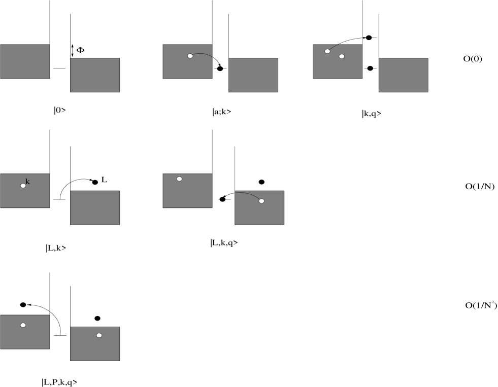
Figure 2: Schematic representation of Hilbert space as organized by the $1/N$ expansion. The diagram shows the succesive electronic transitions due both to the coupling of the dot levels to the leads and the applied bias. Particle-hole excitations are produced in both leads. Sectors with increasing number of particle-hole pairs appear at successive orders in the $1/N$ expansion. We retain configurations which are at most of order O($1/N^{2}$). Not shown, but included in the many-body wavefunction, are configurations with two particle-hole pairs in a single lead, or two particles in one lead and two holes in the other lead.

Figure 4: Electric current per spin channel between the left lead and a quantum dot due to application of a large rectangular pulse bias potential. Time is given in units of $\hbar/\Delta$ where $\Delta=0.2$ meV, and current is in units of $e/h$. Here the bias of amplitude $\Phi=5\Delta$ is applied only to the left lead (see Fig. 1), and the level in the dot is held fixed at $\epsilon_{a}=-2\Delta$. The bias is turned on abruptly at time $t=0.5\hbar/\Delta$ and off at time $t=3.5\hbar/\Delta$. In the same plot we compare the non-interacting, spinless case ($N=1$) with the $N=2$ case for both the $U\rightarrow\infty$ limit and for the experimentally relevant value of $U=2$ meV of a SETGoldhaber . The transient response time of the interacting electrons is longer than for non-interacting electrons. As can be seen upon comparison with the time scales (horizontal lines) the period of the oscillations also increases as $N$ changes from 1 to 2, in accord with the formula $t_{p}={2\pi\hbar\over|\Phi-\epsilon_{a}|}$ but only if we set $\epsilon_{a}=0$ in the case of spinning electrons.

Figure 6: Electric current per spin channel between the left lead and the quantum dot for different dot level energies. Time is in units of $\hbar/\Delta$ where $\Delta=0.2$ meV, and current is in units of $e/h$. We fix $N=2$ and $U=2$ meV, values appropriate for a semiconducting quantum dot. A rectangular pulse bias potential of amplitude $\Phi=5\Delta$ is applied with the dot level set at: $\epsilon_{a}=-3\Delta$, $-2\Delta$, and $-0.5\Delta$. The pulse is abruptly turned on at time $t=0.5\hbar/\Delta$ and off at time $t=3.5\hbar/\Delta$ as marked by the arrows. We find that the period of the oscillations remains constant even as the quantum dot level is moved from the Kondo into the mixed-valence regime. As $\epsilon_{a}/\Delta$ becomes more negative the Kondo scale decreases and the magnitude of the current is also suppressed.

Figure 7: Temperature dependence of the response current per spin channel through a quantum dot. Noninteracting spinless ($N=1$) electrons are compared to interacting spinful electrons ($N=2$). Time is in units of $\hbar/\Delta$ where $\Delta=0.2$ meV, and current is in units of $e/h$. A rectangular pulse bias potential of amplitude $\Phi=5\Delta$ is applied. We set $\epsilon_{a}=-2\Delta$, and for the interacting case we set $U=2$ meV. In contrast to the noninteracting spinless case, for interacting spinful electrons the period of the oscillations and the magnitude of the current decrease significantly as the temperature is increased, approaching those of the spinless system.

References

- (1) A. C. Hewson, The Kondo Problem to Heavy Fermions, (Cambridge University Press 1993).
- (2) D. Goldhaber-Gordon, et al., Phys. Rev. Lett. 81, 5225 (1998); D. Goldhaber-Gordon, et al. Nature 391, 156 (1998); S. M. Cronenwett, et al., Science 281, 540 (1998); J. Schmid, J. Weis, K. Eberl, and K. v. Klitzing, Physica B 256, 182 (1998).
- (3) L. I. Glazman and M. E. Raikh, JETP Lett. 47, 452 (1988); T.-K. Ng and P. A. Lee, Phys. Rev. Lett. 61, 1768 (1988); A. L. Yeyati, A. Martín-Rodero, and F. Flores, Phys. Rev. Lett. 71, 2991 (1993).
- (4) N. S. Wingreen and Y. Meir, Phys. Rev. B 49, 11040 (1994).
- (5) R. M. Konik, H. Saleur, and A. Ludwig, Phys. Rev. B 66, 125304 (2002).
- (6) A. Schiller and S. Hershfield, Phys. Rev. Lett. 77, 1821 (1996); A. Schiller, and S. Hershfield, Phys. Rev. B 62, R16271 (2000).
- (7) P. Nordlander, N. S. Wingreen, Y. Meir, and D. C. Langreth, Phys. Rev. Lett. 83, 808 (1999); M. Plihal, D. C. Langreth, and P. Nordlander, cond-mat/0108525.
- (8) M. Plihal, D. C. Langreth, P. Nordlander, Phys. Rev. B 61, R13341 (2000).
- (9) A. Kaminski, Yu. V. Nazarov, and L. I. Glazman, Phys. Rev. Lett. 83, 384 (1999).
- (10) V. I. Talyanskii, J. M. Shilton, M. Pepper, C. G. Smith, C. J. B. Ford, E. H. Linfield, D. A. Ritchie, and G. A. C. Jones, Phys. Rev. B 56, 15180 (1997).
- (11) G. Cuniberti, M. Sassetti, and B. Kramer, Phys. Rev. B 57, 1515 (1998).
- (12) N. S. Wingreen, A-P Jauho, and Y. Meir, Phys. Rev. B 48, R8487 (1993); A. P. Jauho, N. S. Wingreen, and Y. Meir, Phys. Rev. B 50, 5528 (1994).
- (13) T-K. Ng, Phys. Rev. Lett. 76, 487 (1996).
- (14) J. M. Elzerman, S. D. Franceschi, D. Goldhaber-Gordon, W. G. van der Wiel, and L. P. Kouwenhoven, J. Low Temp. Phys. 118, 375 (2000).
- (15) R. López, R. Aguado, G. Platero, and C. Tejedor, Phys. Rev. Lett. 81, 4688 (1998).
- (16) M. H. Hettler and H. Schoeller, Phys. Rev. Lett. 74, 4907 (1995).
- (17) T. A. Costi, J. Kroha, and P. Wölfle, Phys Rev. B 53, 1850 (1996).
- (18) T. A. Costi, A. C. Hewson, and V. Zlatić, J. Phys: Cond. Matt. 6, 2519 (1994).
- (19) H. Schoeller and J. König, Phys. Rev. Lett. 84, 3686 (2000).
- (20) A. Rosch, J. Paaske, J. Kroha, and P. Wölfle, Phys. Rev. Lett. 90, 076804 (2003).
- (21) M. A. Cazalilla and J. B. Marston, Phys. Rev. Lett. 88, 256403 (2002).
- (22) J. König, Quantum Fluctuations in the Single-Electron Transistor (Shaker Verlag, Aachen, 1999).
- (23) C. M. Varma and Y. Yafet, Phys. Rev. B 13, 2950 (1976); O. Gunnarsson and K. Schönhammer, Phys. Rev. B 28, 4315 (1983).
- (24) O. Gunnarsson and K. Schönhammer, Handbook on the Physics and Chemistry of Rare Earths , Vol. 10 (Elsevier Science Publishers 1987), p. 127.
- (25) R. Brako and D. M. Newns, Solid State Commun. 55, 633 (1985).
- (26) J. B. Marston, D. R. Andersson, E. R. Behringer, B. H. Cooper, C. A DiRubio, G. A. Kimmel, and C. Richardson, Phys. Rev. B 48, 7809 (1993).
- (27) A. V. Onufriev and J. B. Marston, Phys. Rev. B 53, 13 340 (1996).
- (28) J. Merino and J. B. Marston, Phys. Rev. B 58, 6982 (1998).
- (29) G. Toulouse, Proc. Int. School Phys. “Enrico Fermi” LVIII ed. F. O. Goodman in Dynamic Aspects of Surface Physics (1974).
- (30) H. Shao, P. Nordlander, and D. C. Langreth, Phys. Rev. Lett. 77, 948 (1996).
- (31) N. E. Bickers, Rev. Mod. Phys. 59, 845 (1987); T. Matsuura, A. Tsuruta, Y. Ono and Y. Kuroda, J. Phys. Soc. Jap. 66, 1245 (1997).
- (32) J. Göres, D. Goldhaber-Gordon, S. Heemeyer, M. A. Kastner, H. Shtrikman, D. Mahalu, and U. Meirav, Phys. Rev. B 62, 2188 (2000).
- (33) K. L. Sebastian, Phys. Rev. B 31, 6976 (1985).
- (34) F. D. M. Haldane, Phys. Rev. Lett. 40, 416 (1978) (endnote 10); errata Phys. Rev. Lett. 40, 911 (1978).
- (35) Y. Nakamura, Y. A. Pashkin, and J. S. Tsai, Nature 398, 786 (1999).
- (36) P. Coleman, C. Hooley, and O. Parcollet, Phys. Rev. Lett. 86, 4088 (2001).
- (37) A. Rosch, J. Kroha, and P. Wolfle, Phys. Rev. Lett. 87, 156802 (2001).
- (38) M. H. Hettler, J. Kroha, and S. Hershfield, Phys. Rev. B 58, 5649 (1998).
- (39) R. Aguado and D. C. Langreth, Phys. Rev. Lett. 85, 1946 (2000).
- (40) B. A. Jones and C. M. Varma, Phys. Rev. Lett. 58, 843 (1987); B. A. Jones, C. M. Varma, and J. W. Wilkins, Phys. Rev. Lett. 61, 125 (1988).
- (41) I. Affleck and A. W. W. Ludwig, Phys. Rev. Lett. 68, 1046 (1992).
- (42) A. Georges and Y. Meir, Phys. Rev. Lett. 82, 3508 (1999).