Aging dynamics of heterogeneous spin models

Abstract

We investigate numerically the dynamics of three different spin models in the aging regime. Each of these models is meant to be representative of a distinct class of aging behavior: coarsening systems, discontinuous spin glasses, and continuous spin glasses. In order to study dynamic heterogeneities induced by quenched disorder, we consider single-spin observables for a given disorder realization. In some simple cases we are able to provide analytical predictions for single-spin response and correlation functions.

The results strongly depend upon the model considered. It turns out that, by comparing the slow evolution of a few different degrees of freedom, one can distinguish between different dynamic classes. As a conclusion we present the general properties which can be induced from our results, and discuss their relation with thermometric arguments.

1 Introduction

Physical systems with an extremely slow relaxation dynamics (aging) are, at the same time, ubiquitous and fascinating [1]. Much of the insight we have on such systems comes from the study of mean-field models [2].

One of the weak points of the results obtained so far is that they focus on global quantities, e.g. the correlation and response functions averaged over all the spins. On the other hand, we expect one of the peculiar features of glassy dynamics to be its heterogeneity [3, 4, 5, 6, 7, 8, 9, 10, 11]. In order to understand this character, we study the out-of-equilibrium dynamics of three models belonging to three different families of slowly evolving systems: coarsening systems, discontinuous and continuous glasses.

The correlation and response functions of a particular spin depend (among the other things) upon its local environment, i.e. the strength of its interactions with other spins. However, the way the single-spin dynamics is influenced by its environment is highly dependent upon the nature of the system as a whole. For instance, as we will show, while in coarsening systems strongly interacting spins relax faster, for discontinuous glasses the opposite happens. Continuous glasses lie somehow midway. In principle, this allows to distinguish different types of slow dynamics just by looking at the relation between a couple of spins.

The local environment is not the only source of heterogeneities [12, 13, 14]. Even in systems without quenched disorder, like structural glasses, the thermal noise is able to break the initial spatial uniformity and to bring the system in a strongly heterogeneous configuration [3, 4, 5]. Nevertheless we think that considering systems with quenched disorder can be an instructive first step even in that direction. As it has been argued several times [15, 16], structural glasses behaves similarly to some disordered systems because of a sort of self-induced disorder. Each molecule relaxes in the amorphous environment produced by the (partially frozen) arrangement of the other ones.

In order to extract quenched-disorder-induced heterogeneities we will average on a very large number of independent thermal histories. This will delete the effects of the thermal noise.

On the contrary we are forced not to perform a naive average over the disorder realizations, because this would wash any difference between spins. Instead of doing more careful disorder averages, e.g. conditioning on the local environment of the spin under study, we prefer to work with a unique fixed disorder realization. In the limit of large system size we expect local quantities still to fluctuate from site to site, and to converge in distribution sense, making the analysis of a single typical sample representative of the whole ensemble.

After these preliminaries, we can summarize the approach used in this work. Given a disordered model, we take a few typical samples (as big as possible according to our numerical capabilities) from the ensemble and we repeat a huge number of times the typical numerical experiment used for studying out-of-equilibrium dynamics: start from a random configuration, quench the system to a low temperature, where it evolves slowly, wait a time $t_{w}$, switch on a small perturbing field, and take measurements. The observables we measure are local quantities, like single-spin correlation and response functions, averaged over the thermal noise.

We shall consider three different disordered models:

• a two-dimensional ferromagnetic Ising model (couplings are all ferromagnetic but of different strengths), which has a ferromagnetic phase below the critical temperature;

• the 3-spin Ising model on random hypergraph, which has a glassy phase with one step of replica symmetry breaking (1RSB);

• the spin glass Ising model on random graph, also known as Viana-Bray (VB) model [17], which is believed to have a glassy phase with continuous replica symmetry breaking (FRSB).

The last two models are examples of diluted mean-field spin glasses. They lack of any finite-dimensional geometric structure: this makes them soluble using mean-field techniques. On the other hand, the local fluctuations of quenched disorder are not averaged out as in completely connected models. For instance, the local connectivity is a Poissonian random variable. Because of these two features, they are an interesting playing ground for understanding heterogeneous dynamics.

Diluted mean-field models have been intensively studied in the last years, one of the qualifying motivations being their correspondence with random combinatorial problems [18]. Statical heterogeneities have been well understood, at least at 1RSB level. Throughout the paper we shall neglect FRSB effects [19], and assume that 1RSB is a good approximation. In Refs. [20, 21], the authors defined a linear-time algorithm that computes single-spin static quantities for a given sample in 1RSB approximation. The algorithm was dubbed surveys propagation (SP) and, strictly speaking, was defined for computing zero-temperature quantities. It is straightforward, although computationally more demanding, to generalize it for finite temperatures $T$ (the generalization follows the ideas of Ref. [22]): we shall call this generalization SP_T.

The resulting heterogeneities can be characterized by a local Edwards-Anderson parameter. This can be defined [23] by considering $m$ weakly-coupled “clones” $\{\sigma^{(1)},\dots,\sigma^{(m)}\}$ of the system. The local overlap between two of them $q_{\rm\scriptscriptstyle EA}^{(i)}(m)=\langle\sigma_{i}^{(a)}\sigma_{i}^{(b)}\rangle$, with $a\neq b$, is given by

$$q_{\rm\scriptscriptstyle EA}^{(i)}(m)\equiv\frac{1}{Z_{m}}\sum_{\alpha\in\{{\rm states}\}}\!\!e^{-\beta mF_{\alpha}}\,\langle\sigma_{i}\rangle_{\alpha}^{2}\,,$$ (1.1)

where the sum on $\alpha$ runs over the pure states, $\langle\cdot\rangle_{\alpha}$ denotes the thermal average over one of such states, and $Z_{m}=\sum_{\alpha}e^{-\beta mF_{\alpha}}$. Equation (1.1) follows from the observation that the $m$ clones stay at any time in the same state $\alpha$, and that each state is selected with probability $e^{-\beta mF_{\alpha}}/Z_{m}$. The parameter $m$ enables us to select metastable states. In fact we expect the dynamics of discontinuous glasses to be tightly related with the properties of high-energy metastable states [24, 25].

While in a paramagnetic phase $q_{\rm\scriptscriptstyle EA}^{(i)}(m)=0$ apart for a non-extensive subset of the spins, in the spin glass phase $q_{\rm\scriptscriptstyle EA}^{(i)}(m)>0$ in a finite fraction of the system. In general $q_{\rm\scriptscriptstyle EA}^{(i)}(m)$ depends upon the site $i$: the phase is heterogeneous. We will return in the next Section on the dynamical significance of this and other statical results.

The paper is organized as follows. In Sec. 2 we present some of the theoretical expectations which we are going to test. We also give a few technical details concerning the numerics. Section 3 deals with coarsening systems. We postulate the general behavior of response and correlation functions, and test our predictions on a simple model. In Secs. 4 and 5 we present our numerical results for, respectively, the 3-spin and 2-spin interaction spin glasses on random (hyper)graphs. The particularly easy case of weakly interacting spins is treated in Sec. 6. We show that the aging behavior of these spins can be computed from the behavior of their neighbors. Finally, in Sec. 7, we discuss the general picture which emerges from our observations. In Sec. 8 we interpret some of these properties using thermometric arguments. Appendix A present some calculations for coarsening dynamics. A brief account of our results has appeared in Ref. [26].

2 Generalities

In the following we shall discuss three different spin models. Before embarking in such a tour it is worth presenting the general frame and fixing some notations.

Our principal tools will be the single-spin correlation and response functions:

$$C_{ij}(t,t_{w})\equiv\langle\sigma_{i}(t)\sigma_{j}(t_{w})\rangle\,,\;\;\;\;\;\;\;R_{ij}(t,t_{w})\equiv\left.\frac{\partial\langle\sigma_{i}(t)\rangle}{\partial h_{j}(t_{w})}\right|_{h=0}\,,$$ (2.1)

where the average is taken with respect to some stochastic dynamics, and $h_{j}$ is a magnetic field coupled to the spin $j$. It is also useful to define the integrated response $\chi_{ij}(t,t_{w})=\int_{t_{w}}^{t}\!ds\,R_{ij}(t,s)$.

We shall not repeat the subscripts when considering the diagonal elements of the above functions (i.e. we shall write $C_{i}$ for $C_{ii}$, etc.). The global (self-averaging) correlation and response functions are obtained from the single-site quantities as follows: $C(t,t_{w})=(1/N)\sum_{i}C_{i}(t,t_{w})$; $\chi(t,t_{w})=(1/N)\sum_{i}\chi_{i}(t,t_{w})$. The times $t$ and $t_{w}$ are measured with respect to the initial quench (at $t_{\rm quench}=0$) from infinite temperature.

We will be interested in comparing the outcome of static calculations and out-of-equilibrium numerical simulations. For instance, we expect the order parameter (1.1) to have the following dynamical meaning

$$q_{\rm\scriptscriptstyle EA}^{(i)}(m_{\rm th})=\lim_{\Delta t\to\infty}\lim_{t_{w}\to\infty}C_{i}(t_{w}+\Delta t,t_{w})\,,$$ (2.2)

where $m_{\rm th}$ is the parameter which select the highest energy metastable states.

In the aging regime $\Delta t,t_{w}\gg 1$, $C_{i}(t_{w}+\Delta t,t_{w})<q_{\rm\scriptscriptstyle EA}^{(i)}(m_{\rm th})$. We expect the functions (2.1) to satisfy the out-of-equilibrium fluctuation-dissipation relation (OFDR) [24]

$$TR_{i}(t,t_{w})=X_{i}[C_{i}(t,t_{w})]\partial_{t_{w}}C_{i}(t,t_{w})\,.$$ (2.3)

If $X_{i}[C_{i}]=1$ the fluctuation-dissipation theorem (FDT) is recovered. The arguments of Refs. [27, 28], and the analogy with exactly soluble models [24, 29, 30] suggest that the function $X_{i}[C]$ is related to the static overlap probability distribution:

$$P_{i}(q)=-\frac{dX_{i}(q)}{dq}\,.$$ (2.4)

For discontinuous glasses the dynamics never approaches thermodynamically dominant states. In this case the function $P_{i}(q)$ entering in Eq. (2.4) is the overlap distribution among highest metastable states. We refer to the next Sections for concrete examples of the general relation (2.4).

Let us now give some details concerning our numerical simulations. We shall consider systems defined on $N$ Ising spins $\sigma_{i}=\pm 1$, $i\in\{1,\dots,N\}$, with Hamiltonian $H(\sigma)$. The dynamics is defined by single spin flip moves with Metropolis acceptance rule. The update will be sequential for the spin glass models of Secs. 4 and 5 and random sequential for the ferromagnetic model of Sec. 3.

For each one of the mentioned models, we shall repeat the typical aging “experiment”. The system is initialized in a random (infinite temperature) configuration. At time $t_{\rm quench}=0$, the system is cooled at temperature $T$ within its low temperature phase. We run the dynamics for a “physical” time $t_{w}$ (corresponding to $t_{w}$ attempts to flip each spin). Then we “turn on” a small random magnetic field $h_{i}=\pm h_{0}$ and go on running the Metropolis algorithm for a maximum physical time $\Delta t_{\rm MAX}$. Notice that the random external field is changed at each trajectory.

The correlation and response of the single degrees of freedom are extracted by measuring the following observables:

$$C_{i}(t_{w}+2\Delta t,t_{w}|h_{0}) \equiv \frac{1}{\Delta t}\sum_{t^{\prime}=t_{w}+\Delta t+1}^{t_{w}+2\Delta t}\langle\sigma_{i}(t^{\prime})\sigma_{i}(t_{w})\rangle\,,$$ (2.5)

$$\chi_{i}(t_{w}+2\Delta t,t_{w}|h_{0}) \equiv \frac{1}{\Delta t\,h_{0}}\sum_{t^{\prime}=t_{w}+\Delta t+1}^{t_{w}+2\Delta t}\langle\sigma_{i}(t^{\prime})\,{\rm sign}(h_{i})\rangle\,,$$ (2.6)

where $\langle\cdot\rangle$ denotes the average over the Metropolis trajectories and the random external field. The sum over $t^{\prime}$ has been introduced for reducing the statistical errors. While it is a drastic modification of the definition (2.1) in the quasi-equilibrium regime $\Delta t\ll t_{w}$, it produces just a small correction in the aging regime $\Delta t,t_{w}\gg 1$. This correction should cancel out in two interesting cases: $(i)$ in the time sector $t/t_{w}={\rm const.}$, if one restrict himself to the response-versus-correlation relation; $(ii)$ in “slower” time sectors (e.g. $(\log t)^{\mu}-(\log t_{w})^{\mu}={\rm const.}$, with $\mu<1$). The functions (2.5) and (2.6) have finite $h_{0}\to 0$ limits $C_{i}(t_{w}+\Delta t,t_{w})$ and $\chi_{i}(t_{w}+\Delta t,t_{w})$.

Finally, let us mention that we shall look at the $\chi_{i}(t,t_{w})$ versus $C_{i}(t,t_{w})$ data from two different perspectives. In the first one we focus on a fixed site $i$ and vary the times $t$ and $t_{w}$: this allows to verify the relations (2.3) and (2.4). We shall refer to this type of presentations as FD plots. In the second approach we plot, for a given couple of times, all the points $(C_{i}(t,t_{w}),\chi_{i}(t,t_{w}))$ for $i=1,\dots,N$. Then we let $t$ grow as $t_{w}$ is kept fixed. We dubbed such a procedure a movie plot. It emphasizes the relations between different degrees of freedom in the system.

3 Coarsening systems

Coarsening is the simplest type of aging dynamics [32, 31]. Despite its simplicity it has many representatives: ferromagnets (both homogeneous and not), binary liquids, and, according to the droplet model [33, 34, 35, 36], spin glasses.

Consider a homogeneous spin model with a low temperature ferromagnetic phase (e.g. an Ising model in dimension $d\geq 2$). When cooled below its critical temperature, the system quickly separates into domains of different magnetization. Within each domain the system is “near” one of its equilibrium pure phases. Nevertheless it keeps evolving at all times due the the growth of the domain size $\xi(t)$. This process is mainly driven by the energetics of domain boundaries.

In the $t\to\infty$ limit, the coarsening length obeys a power law $\xi(t)\sim t^{1/z}$ (for non-conserved scalar order parameter $z=2$). Two-times observables decompose in a quasi-equilibrium part describing the fluctuations within a domain ($C_{\rm eq}$ and $\chi_{\rm eq}$ in the equations below), plus an aging contribution which involves the motion of the domain walls ($C_{\rm ag}$, $C_{\rm dw}$ and $\chi_{\rm dw}$):

$$C(t,t_{w}) \approx C_{\rm eq}(t-t_{w})+q_{\rm\scriptscriptstyle EA}C_{\rm ag}\left(\frac{\xi(t)}{\xi(t_{w})}\right)-q_{\rm\scriptscriptstyle EA}t_{w}^{-a}C_{\rm dw}\left(\frac{\xi(t)}{\xi(t_{w})}\right)\,,$$ (3.1)

$$\chi(t,t_{w}) \approx \chi_{\rm eq}(t-t_{w})+\phantom{q_{\rm\scriptscriptstyle EA}C_{\rm ag}\left(\frac{\xi(t)}{\xi(t_{w})}\right)}+q_{\rm\scriptscriptstyle EA}t_{w}^{-a^{\prime}}\chi_{\rm dw}\left(\frac{\xi(t)}{\xi(t_{w})}\right)\,,$$ (3.2)

where $q_{\rm EA}$ is the equilibrium Edwards-Anderson parameter. For a ferromagnet $q_{\rm EA}=M(\beta)^{2}$, $M(\beta)$ being the spontaneous magnetization. Moreover $C_{\rm eq}(\tau)$ decreases from $(1-q_{\rm EA})$ to $0$ as $\tau$ goes from $0$ to $\infty$, and $C_{\rm ag}(\lambda)$ goes from $1$ to $0$ as its argument increases from $1$ to $\infty$. Finally the equilibrium part of the susceptibility $\chi_{\rm eq}(\tau)$ goes from $0$ to $(1-q_{\rm EA})/T$. In the case of a scalar order parameter both the response and correlation functions receive subleading contributions ($C_{\rm dw}$ and $\chi_{\rm dw}$) from spins “close” to the domain walls. Notice that these spins will decorrelate faster and respond easier than the others (in other words $C_{\rm dw}$ and $\chi_{\rm dw}$ are typically positive). These contributions are expected to be proportional to the density of domain walls $\rho_{\rm dw}(t_{w})\propto\xi(t_{w})^{-1}$. This would imply $a=a^{\prime}=1/z$.

It is easy to generalize this well-established scenario to include single-spin quantities in heterogeneous systems. We expect that the quasi-equilibrium parts of the correlation and response functions will depend upon the detailed environment of each spin. On the other hand, the large scale motion of the domain boundaries will not depend upon the precise point of the system we are looking at. Therefore the aging contribution will depend upon the site $x$ only through the local Edwards-Anderson parameter $q^{\rm\scriptscriptstyle EA}_{x}=M_{x}(\beta)^{2}$. The reason is that $q^{\rm\scriptscriptstyle EA}_{x}$ quantifies the distance between pure phases as seen through the spin $\sigma_{x}$.

We are led to propose the following form for single-site functions:

$$C_{x}(t,t_{w}) \approx C_{x}^{\rm eq}(t-t_{w})+q^{\rm\scriptscriptstyle EA}_{x}C_{\rm ag}\left(\frac{\xi(t)}{\xi(t_{w})}\right)-q^{\rm\scriptscriptstyle EA}_{x}t_{w}^{-a}C_{\rm dw}\left(\frac{\xi(t)}{\xi(t_{w})}\right)\,,$$ (3.3)

$$\chi_{x}(t,t_{w}) \approx \chi_{x}^{\rm eq}(t-t_{w})+\phantom{q^{\rm\scriptscriptstyle EA}_{x}C_{\rm ag}\left(\frac{\xi(t)}{\xi(t_{w})}\right)}+q^{\rm\scriptscriptstyle EA}_{x}t_{w}^{-a^{\prime}}\chi_{\rm dw}\left(\frac{\xi(t)}{\xi(t_{w})}\right)\,.$$ (3.4)

This ansatz can be summarized, as far as $O(t_{w}^{-a},t_{w}^{-a^{\prime}})$ terms are neglected, in the schematic response-versus-correlation plot reported in Fig. 1. Each spin follows its own fluctuation-dissipation curve. This is composed by a quasi-equilibrium sector $T\chi_{x}=1-C_{x}$, plus an horizontal aging sector $T\chi_{x}=1-q^{\rm\scriptscriptstyle EA}_{x}$. Moreover, for each couple of times $t_{w}$ and $t$, all the points are aligned on the line passing through $(C=0,T\chi=1)$.

Figure 1: Qualitative picture of the response-versus-correlation plot for coarsening systems. Bold dashed lines are the single-spin OFDR’s. Black dots represent the correlation and response functions at a given pairs of times $(t,t_{w})$. Arrows correspond to the “velocities” of the dots when they move along the fluctuation-dissipation curves.

Notice that spins with larger $q^{\rm\scriptscriptstyle EA}_{x}$ relax faster. Roughly speaking this happens because they have to move a larger distance in order to jump from one pure phase to the other.

Due to the independence of $C_{\rm dw}$ and $\chi_{\rm dw}$ upon the site $x$, Eqs. (3.3) and (3.4) imply that alignment in the $\chi$-$C$ plane is verified even in the pre-asymptotic regime. This property is therefore more robust than the OFDR which is violated by $O(t_{w}^{-a},t_{w}^{-a^{\prime}})$ terms, cf. Figs. 4 and 5.

Finally, both the large-$n$ calculation of Sec. 3.1.1, and our numerical data, cf. Sec. 3.1.2, suggest that domain-wall contributions in Eqs. (3.3), (3.4) have the same order of magnitude $C_{\rm dw}(\lambda)\sim T\chi_{\rm dw}(\lambda)$.

3.1 A staggered spin model

Here we want to test our predictions in a simple context. We shall consider a $d$-dimensional lattices ferromagnet, defined by the Hamiltonian

$$H(\sigma)=-\sum_{(xy)}J_{xy}\sigma_{x}\sigma_{y}\,,$$ (3.5)

where the sum runs over all the couples $(xy)$ of nearest-neighbors on the lattice $\mathbb{Z}^{d}$, and $J_{xy}\geq 0$. Moreover we assume periodicity in the couplings. Namely, there exist positive integers $l_{1},\dots,l_{d}$ such that, for any $x,y\in\mathbb{Z}^{d}$, and $\mu\in\{1,\dots,d\}$

$$J_{xy}=J_{x+\hat{\mu}l_{\mu},y+\hat{\mu}l_{\mu}}$$ (3.6)

where $\hat{\mu}$ is the unit vector in the $\mu$-th direction. Clearly there are $V=l_{1}\cdot l_{2}\cdots l_{d}$ different “types” of spins in this model. Two spins of the same type have the same correlation and response functions. We can identify these $V$ types with the spins of the “elementary cell” $\Lambda\equiv\{x\in\mathbb{Z}^{d}|0\leq x_{\mu}<l_{\mu}\}$.

Spatial periodicity is helpful for two reasons: $(i)$ it allows an analytical treatment in the large-$n$ limit; $(ii)$ averaging the single-spin quantities over the set of spins of a given type greatly improves the statistics of numerical simulations.

3.1.1 Large $n$

The model (3.5) is easily generalized to $n$-vector spins $\mbox{\boldmath$\phi$}_{x}=(\phi^{1}_{x},\dots,\phi^{n}_{x})$. We just replace the ordinary product between spins in Eq. (3.5) with the scalar product. Moreover we fix the spin length: $\mbox{\boldmath$\phi$}_{x}\cdot\mbox{\boldmath$\phi$}_{x}=n$. The dynamics is specified by the Langevin equation:

$$\partial_{t}\phi^{a}_{x}(t)=-\zeta_{x}(t)\phi^{a}_{x}(t)+\sum_{y}J_{xy}\phi^{a}_{y}(t)+\eta^{a}_{x}(t)\,,$$ (3.7)

where we introduced the Lagrange multipliers $\zeta_{x}(t)$ in order to enforce the spherical constraint. The thermal noise is Gaussian with covariance

$$\langle\eta^{a}_{x}(t)\eta^{b}_{y}(s)\rangle=2T\delta_{xy}\delta^{ab}\delta(t-s)\,.$$ (3.8)

The definition of correlation and response functions must be slightly modified for an $n$-components order parameter:

$$C_{xy}(t,t^{\prime})=\frac{1}{n}\langle\mbox{\boldmath$\phi$}_{x}(t)\cdot\mbox{\boldmath$\phi$}_{y}(t^{\prime})\rangle\,,\;\;\;\;\;\;\;\;R_{xy}(t,t^{\prime})=\frac{1}{n}\sum_{a}\frac{\delta\langle\phi^{a}_{x}(t)\rangle}{\delta h_{y}^{a}(t^{\prime})}\,.$$ (3.9)

Like its homogeneous relative [31], this model can be solved in the limit $n\to\infty$. The calculations are outlined in App. A. Let’s summarize here the main results. For $d>2$ the model undergoes a phase transition at a finite temperature $T_{c}$. Below the critical temperature the $O(n)$ symmetry is broken: $\langle\phi_{x}^{a}\rangle=M_{x}(\beta)\delta^{a1}$. Of course the spontaneous magnetizations preserves the spatial periodicity of the model: $M_{x+l_{\mu}\hat{\mu}}(\beta)=M_{x}(\beta)$.

Figure 2: Domain wall contributions to the correlation (dashed line) and integrated response functions (continuous line) in the $n\to\infty$ limit: the universal scaling functions, cf. Eqs. (3.11) and (3.12), as a function of $\lambda=\sqrt{t/t_{w}}$.

At low temperature, the forms (3.3)-(3.4) hold, with $q_{x}^{\rm EA}=M^{2}_{x}(\beta)$, $a=a^{\prime}=d/2-1$, $z=2$ and

$$C_{\rm ag}(\lambda) = \left(\frac{\lambda+\lambda^{-1}}{2}\right)^{-d/2}\,.$$ (3.10)

The subleading contribution read

$$C_{\rm dw}(\lambda) = \frac{2T}{(8\pi)^{d/2}(\sum_{x\in\Lambda}M_{x}^{2})\Delta^{1/2}}\cdot{\cal F}_{C}(\lambda;d)\,,$$ (3.11)

$$\chi_{\rm dw}(\lambda) = \frac{2}{(4\pi)^{d/2}(\sum_{x\in\Lambda}M_{x}^{2})\Delta^{1/2}}\cdot{\cal F}_{\chi}(\lambda;d)\,,$$ (3.12)

where $\Delta$ is a constant which depends uniquely on the couplings $J_{xy}$, cf. App. A.1. ${\cal F}_{C}(\cdot)$, ${\cal F}_{\chi}(\cdot)$ are two universal function which do not depend either on the temperature or on the particular model. The explicit expressions for these functions are not very illuminating. We report them in App. A.2, see Eqs. (A.18) and (A.19). Here we plot the two functions in the $d=3$ case, see Fig. 2. Notice that both ${\cal F}_{C}(\lambda;d)$ and ${\cal F}_{\chi}(\lambda;d)$ vanish in the $\lambda\to\infty$ limit. This could be expected because we know that $C_{x}(t,t_{w})\to 0$ and $\chi_{x}(t,t_{w})\to(1-M_{x}^{2})/T$ as $t\to\infty$ for any fixed $t_{w}$.

3.1.2 Numerical simulations

We simulated the model (3.5) in $d=2$ dimensions with $l_{1}=l_{2}=2$ and the choice of couplings among spins in the elementary cell illustrated in Fig. 3. We used square lattices with linear size $L$. There are $V=2^{2}$ different type of spins in this case. We shall improve our numerical estimates by averaging the single site functions $C_{i}(t,t_{w};h_{0})$ and $\chi_{i}(t,t_{w};h_{0})$, cf. Eqs. (2.5) and (2.5), over the $L^{2}/4$ spins of the same type.

Figure 3: Definition of the ferromagnetic couplings for the two-dimensional model studied in Sec. 3.1.2.

Most our numerical results were obtained at temperature $T=1$. A rough numerical estimate yields $T_{c}=1.10(5)$ for the critical temperature. The equilibrium magnetizations for $T=1$ of the four type of sites are: $M_{0}=0.8803(5)$, $M_{1}=0.8395(5)$, $M_{2}=0.7573(5)$, and $M_{3}=0.8624(5)$. Notice that, in order to separate the magnetization values on different sites, we are forced to choose a quite high temperature for our simulations.

We expect the growth of the domain size in the model (3.5) to follow asymptotically the law $\xi(t)\approx k(\beta)\cdot t^{1/z}$, with $z=2$, as in the homogeneous case. The pinning effect due to inhomogeneous couplings will renormalize the coefficient $k(\beta)$. We checked this law by studying the evolution of the total magnetization starting from a random initial condition for different lattice sizes. It turns out that the law is reasonably well verified with a coefficient $k(\beta=1)$ of order one.

The aging “experiment” was repeated for several values of the waiting time $t_{w}=10$, $10^{2}$, $10^{3}$, $10^{4}$, $10^{5}$. The correlation and response functions were measured up to a maximum time interval (respectively) $\Delta t_{\rm MAX}=2^{10}$, $2^{13}$, $2^{15}$, $2^{17}$, $2^{19}$. The linear size of the lattice was $L=2000$ in all the cases except for $t_{w}=10^{5}$. In this case we used $L=1000$. All the results were therefore obtained in the $\xi(t)\ll L$ regime, with the exception, possibly, of the latest times in the $t_{w}=10^{5}$ run. Some systematic discrepancies can be indeed noticed for these data. In the Table below we report the number $N_{\rm stat}$ of different runs for each choice of the parameters.

$h_{0}$	$t_{w}=10$	$t_{w}=10^{2}$	$t_{w}=10^{3}$	$t_{w}=10^{4}$	$t_{w}=10^{5}$
$0.025$	$30$	$23$	$30$	$9$	$\star$
$0.05$	$30$	$12$	$12$	$5$	$10$
$0.10$	$\star$	$\star$	$\star$	$12$	$\star$

Let us start by illustrating how the asymptotic behavior summarized in Fig. 1 is approached. In Fig. 4 we show the correlation functions and the FD plot for type-0 sites. Notice that the approach to the asymptotic behavior is quite slow and, in particular, the domain-wall contribution to the response function is pretty large. This can be an effect of the proximity of the critical temperature: the “thickness” of the domain walls grows with the equilibrium correlation length.

Figure 4: Correlation function and FD plot for type-0 sites (cf. Fig. 3). Different symbols correspond to $t_{w}=10$ ($\Box$), $10^{2}$ ($\ast$), $10^{3}$ ($\times$), $10^{4}$ ($+$), $10^{5}$ (filled $\Box$). The dot-dashed line on the left is the equilibrium Edwards-Anderson parameter $M_{0}^{2}$. On the right we report the FDT line $T\chi=1-C$ (dot-dashed) and the OFDR (dashed) which corresponds to Eqs. (3.3) and (3.4).

Figure 5: Movie plots at $t_{w}=10^{3}$ (left) and $10^{4}$ (right). The various symbols correspond to different types of spin: type 0 ($+$), type 1 ($\times$), type 2 ($\Box$), and type 3 ($\ast$). The straight lines confirm the alignment predicted in the general picture, cf. Fig. 1.

In Fig. 5 we verify the alignment of different sites correlation and response functions for a given pair of times $(t,t_{w})$.

Figure 6: Correlation function (left) and FD plot (right) with the rescaled correlation and response functions, see Eq. (3.13), for all the four spin types and several different waiting times: $t_{w}=10^{2}$, $10^{3}$, $10^{4}$, and, on the left $10^{5}$. Here $h_{0}=0.05$.

Notice that the alignment works quite well even for “pre-asymptotic” times, i.e. when the anomalous response is still sizeable and the OFDR is not well verified, cf. Fig. 4.

Figure 7: The fitting temperature (3.14) as a function of $\lambda=\sqrt{t/t_{w}}$ for $t_{w}=10$ (filled $\Box$), $10^{2}$ ($\Box$), $10^{3}$ ($\ast$), $10^{4}$ ($+$), and $10^{5}$ ($\times$). The dot-dashed line is the $n=\infty$ scaling function (3.10), with $d=2$.

In order to check the form (3.4) for the site dependence of the domain wall contribution, we plot in Fig. 6 the rescaled response and correlation functions:

$$C^{\rm res}_{x}=\frac{\overline{q}}{q^{\rm\scriptscriptstyle EA}_{x}}C_{x}\,,\;\;\;T\chi^{\rm res}_{x}=1-\frac{\overline{q}}{q^{\rm\scriptscriptstyle EA}_{x}}(1-T\chi_{x})\,,$$ (3.13)

where $\overline{q}$ is an arbitrary reference overlap. The rescaled correlation and response functions of different types of spin coincide perfectly for any couple of times $(t,t_{w})$.

Finally, we notice that we can consistently define a time-dependent fitting temperature as the slope of the lines in Fig. 5, i.e.:

$$T_{\rm fit}(t,t_{w})=\frac{T\,C_{x}(t,t_{w})}{1-T\chi_{x}(t,t_{w})}\,.$$ (3.14)

As a consequence of Eqs. (3.3) and (3.4) this temperature should depend upon $t$ and $t_{w}$ only through the parameter $\lambda=\xi(t)/\xi(t_{w})$. In Fig. 7 we verify this scaling.

4 Discontinuous glasses

In this Section we consider a ferromagnetic Ising model with 3-spin interactions, defined on a random hypergraph [37, 38]. More precisely, the Hamiltonian reads

$$H(\sigma)=-\sum_{(ijk)\in{\cal H}}\sigma_{i}\sigma_{j}\sigma_{k}\,.$$ (4.1)

The hypergraph ${\cal H}$ defines which triplets of spins do interact. We construct it by randomly choosing $M$ among the $N(N-1)(N-2)/3!$ possible triplets of spins.

Although ferromagnetic, this model is thought to have a glassy behavior, due to self-induced frustration [39]. Depending upon the value of $\gamma\equiv M/N$, it undergoes no phase transition (if $\gamma<\gamma_{d}$), a purely dynamic phase transition (if $\gamma_{d}<\gamma<\gamma_{c}$), or a dynamic and a static phase transitions (if $\gamma>\gamma_{c}$) as the temperature is lowered. The 1RSB analysis of Refs. [37, 40] yields $\gamma_{d}\approx 0.818$ and $\gamma_{c}\approx 0.918$. These results have been later confirmed by rigorous derivations [41, 42].

We studied two samples extracted from the ensemble defined above: the first one involves $N=100$ sites and $M=100$ interactions (hereafter we shall refer to it as ${\cal H}_{A}$); in the second one (${\cal H}_{B}$) we have $N=M=1000$. In both cases $\gamma=1>\gamma_{c}$. The hypergraph ${\cal H}_{A}$ consists of a large connected component including $96$ sites, plus $4$ isolated sites (namely the sites $i=15,22,62,69$). The largest connected component of ${\cal H}_{B}$ includes $938$ sites (there are $62$ isolated sites). We will illustrate our results mainly on ${\cal H}_{A}$ (on this sample we were able to reach larger waiting times). ${\cal H}_{B}$ has been used to check finite-size effects.

Figure 8: The complexity $\Sigma(T)$ (left) and the 1RSB parameter $m_{\rm th}(T)$ (right) for threshold states as functions of the temperature $T$. These curves refer to sample ${\cal H}_{A}$ considered in Sec. 4.

Using SP_T, we computed the 1RSB free energy density $F(m,\beta)$ and complexity $\Sigma(T)=\beta\,\partial_{m}F(m,\beta)|_{m=1}$ for our samples as a function of the temperature $T=1/\beta$. The resulting complexity is reported in Fig. 8 for sample ${\cal H}_{A}$. The dynamic and static temperatures are defined, respectively, as the points where a non-trivial (1RSB) solution of the cavity equations first appears, and where its complexity vanishes. From the results of Fig. 8 (left frame) we get the estimates $T_{d}=0.557(2)$ and $T_{c}=0.467(2)$.

In analogy with the analytic solution of the $p$-spin spherical model [24, 25], we assume the aging dynamics of the model (4.1) to be dominated by threshold states. These are defined as the 1RSB metastable states with the highest free energy density. Although not exact [19], we expect this assumption to be a good approximation for not-too-high values of $\gamma$. The threshold 1RSB parameter $m_{\rm th}(T)$ can be computed by imposing the condition $\partial_{m}^{2}[mF(m,\beta)]=0$. We computed $m_{\rm th}(T)$ on sample ${\cal H}_{A}$ for a few temperatures below $T_{d}$. We get $m_{\rm th}(0.3)=0.395(10)$, $m_{\rm th}(0.4)=0.58(1)$, $m_{\rm th}(0.5)=0.80(1)$. Moreover, in the zero temperature limit, we obtain $m_{\rm th}(T)=\mu_{\rm th}T+O(T^{2})$, with $\mu_{\rm th}=1.08(1)$. These results are summarized in Fig. 8 (right frame). A good description of the temperature dependence is obtained using the polynomial fit $m_{\rm th}(T)=1.08\,T+0.038\,T^{2}+2.17\,T^{3}$ (cf. continuous line in Fig. 8, right frame).

Now we are in the position of precising the connection between single-spin statics and aging dynamics, outlined in Sec. 2. It is convenient to work with the integrated response functions $\chi_{i}(t,t_{w})$. Equation (2.3) implies the relation $\chi_{i}(t,t_{w})=\chi_{i}[C_{i}(t,t_{w})]$ to hold in the limit $t,t_{w}\to\infty$. Within a 1RSB approximation, Eq. (2.4) corresponds to:

$$T\chi_{i}[q]=\left\{\begin{array}[]{cl}1-q&\mbox{ for $q>q_{\rm\scriptscriptstyle EA,th}^{(i)}$}\,,\\ 1-q_{\rm\scriptscriptstyle EA,th}^{(i)}-m_{\rm th}(q-q_{\rm\scriptscriptstyle EA,th}^{(i)})&\mbox{ for $q<q_{\rm\scriptscriptstyle EA,th}^{(i)}$}\,,\end{array}\right.$$ (4.4)

where we used the shorthand $q_{\rm\scriptscriptstyle EA,th}^{(i)}=q_{\rm\scriptscriptstyle EA}^{(i)}(m_{\rm th})$. Since the SP_T algorithm allows us to compute both $m_{\rm th}$ and the parameters $q_{\rm\scriptscriptstyle EA}^{(i)}(m)$ for a given sample in linear time, we can check the above prediction in our simulations.

4.1 Numerical results

We ran our simulations at three different temperatures ($T=0.3,0.4,0.5$) and intensities of the external field ($h_{0}=0.05,0.1,0.15$). In order to probe the aging regime, we repeated our simulations for several waiting times $t_{w}=10,10^{2},10^{3},10^{4}$, with (respectively) $\Delta t_{\rm MAX}=2^{13},2^{16},2^{16},2^{18}$.

We summarize in the Table below the statistic of our simulations on sample ${\cal H}_{A}$.

$h_{0}$	$t_{w}=10$	$t_{w}=10^{2}$	$t_{w}=10^{3}$	$t_{w}=10^{4}$
$0.05$	$5\cdot 10^{6}$	$5\cdot 10^{6}$	$5\cdot 10^{6}$	$10^{6}$
$0.10$	$1.5\cdot 10^{6}$	$1.5\cdot 10^{6}$	$1.5\cdot 10^{6}$	$10^{6}$
$0.15$	$10^{6}$	$10^{6}$	$10^{6}$	$0.5\cdot 10^{6}$

For sample ${\cal H}_{B}$, we limited ourselves to the case $h_{0}=0.10$, $T=0.4$, and generated $0.9\cdot 10^{6}$ Metropolis trajectories with $t_{w}=10^{3}$.

4.1.1 Two types of spins

The most evident feature of our numerical data, is that the spins can be clearly classified in two groups: (I) the ones which behave as if the system were in equilibrium: the corresponding correlation and response functions satisfy time-traslation invariance and FDT; (II) the out-of-equilibrium spins, whose correlation and response functions are non-homogeneous on long time scales and violate FDT.

Of course the group (I) includes the isolated sites, but also an extensive fraction of non-isolated sites (for instance the $12$ sites $i=1,6,8,14,27,39,68,74,$ $77,84,87,98$ of sample ${\cal H}_{A}$). Remarkably these sites are the ones for which the SP_T algorithm returns $q^{(i)}_{\rm EA}=0$: they are paramagnetic from the static point of view.

Figure 9: Correlation function (left) and FD plot (right) of the spin $i=1$ (sample ${\cal H}_{A}$) for $T=0.5$, $h_{0}=0.1$ and $t_{w}=10\div 10^{4}$. Time-traslation invariance is well verified for $t_{w}\gtrsim 100$. The discrepancy from FDT (continuous line on the right) can be ascribed to nonlinear response effects.

Figure 10: Correlation function (left) and FD plot (right) for the spin $i=0$ (sample ${\cal H}_{A}$). The dashed line on the left corresponds the ergodicity breaking parameter $q_{\rm\scriptscriptstyle EA}^{(i)}=0.716(7)$ obtained with the SP_T algorithm. On the right we report with a full line the corresponding OFDR predicted within a 1RSB scenario.

In Figs. 9 and 10 we present the correlation function and the FD plot, respectively, for a type-I site and a type-II site. In both cases we took $T=0.5$ and $h=0.05$.

There exists a nice geometrical characterization of type-I sites in terms of a leaf-removal algorithm [41, 42]. Let us recall here the definition of this procedure. The algorithm starts by removing all the interactions which involve at least one site with connectivity 1. The same operation is repeated recursively until no connectivity-1 site is left. The reduced graph will contain either isolated sites, or sites which have connectivity greater than one. The sites of this last type are surely type-II, but they are not the only ones. In fact one has to restore a subset of the original interactions according to the following recursive rule. If an interaction involves at least two type-II sites, restore it and declare the third site to be type-II. If no such an interaction can be found among the original ones, stop. In this way, one has singled out the subset of original interactions which are relevant for aging dynamics. The sites which remain isolated after this restoration procedure are type-I sites, the others are type-II.

The dynamical relevance of this construction is easily understood by considering two simple cases. A connectivity-1 spin whose two neighbors evolve slowly will be affected by a slow local field and will relax on the same time-scale of the field. In the opposite case, two connectivity-1 spins whose neighbor evolve slowly will effectively see just a slowly alternating two-spin coupling between them. They will relax as fast as a two-spin isolated cluster does.

Figure 11: The correlation functions of four type-I spins of sample ${\cal H}_{A}$: from above to below $i=1,14,8,15$. The first three sites are connected to the rest of the cluster (and therefore interacting), the last one is isolated (free).

It is worth stressing that the above construction does not contain all the dynamical information on the model. For instance, one may wonder whether the dynamics of type-I spins does resemble to the dynamics of isolated spins. The answer is given in Fig. 11 where we reproduce the correlation functions for several different type-I spins, for $T=0.5$, $h=0.1$ and $t_{w}=10^{4}$ (remember that the dependence upon $t_{w}$ is weak for these sites). The results are strongly site-dependent and by no way similar to the free-spin case. Notice the peculiar behavior of the isolated spin, an artifact of Metropolis algorithm with sequential updatings. Weren’t for the perturbing field we would have $\sigma_{i}(t)=(-1)^{t}\sigma_{i}(0)$, which implies $C_{i}(t_{w}+1,t_{w})=-1$, $C_{i}(t_{w}+2,t_{w})=1$, and $C_{i}(t_{w}+2\Delta t,t_{w})=0$ for $\Delta t\geq 2$ [remind the time average in Eq.(2.5)]. In the presence of an external field the correlation function (with no time-average) becomes $C_{i}(t_{w}+t,t_{w})=[-\exp(-2\beta h)]^{t}$.

Finally, in Fig. 10 we compare the numerical results with the prediction from the statics, cf. Eq. (4.4). The agreement is quite good although finite-$t_{w}$ and finite-$h_{0}$ effects are not negligible.

4.1.2 Dependence on the perturbing field

We claimed that type-I spins satisfy FDT. However the FD plot in Fig. 9 is not completely convincing on this point. The data show a small but significant discrepancy with respect to the FDT-line. We want to show here that this is (at least partially) a finite-$h_{0}$ effect.

In order to have a careful check of this effect, we used, on sample ${\cal H}_{A}$, three different values of $h_{0}$ for any choice of $T$ and $t_{w}$. The main outcome of this analysis is that the $h_{0}$ dependence is much stronger for type-I than for type-II spins. This can be easily understood: type-II spins interact strongly with their neighbors and are therefore “stiffer”.

Figure 12: The fluctuation-dissipation plot for a type-I (left frame: site $i=1$ on ${\cal H}_{A}$) and for a type-II site (right frame: site $i=0$ on ${\cal H}_{A}$) at $T=0.4$. Different symbols refer to different values of the perturbing field: $h_{0}=0.05$ ($\times$), $0.10$ ($\ast$), $0.15$ ($\Box$), and $h_{0}\to 0$ extrapolation (continuous line). The dot-dashed lines refer to the FDT and (in the right frame) the predicted OFDR.

In Fig. 12 we present the FD plots for two sites of sample ${\cal H}_{A}$: $i=1$ (type-I) and $i=0$ (type-II), and the three values of $h_{0}$ used in simulations. We expect the correlation and response functions to approach the zero-field limit as follows:

$$C_{i}(t,t_{w}|h_{0})=C_{i}(t,t_{w})+D_{i}(t,t_{w})\,h_{0}^{2}+O(h_{0}^{4})\,,$$ (4.5)

$$\chi_{i}(t,t_{w}|h_{0})=\chi_{i}(t,t_{w})+\delta_{i}(t,t_{w})\,h_{0}^{2}+O(h_{0}^{4})\,.$$ (4.6)

We fitted our numerical data using the above expressions (and neglecting next-to-leading corrections). The results of this extrapolation are reported in Fig. 12 together with the finite-$h_{0}$ data.

As can be verified on Fig. 12, for type-II spins the $h_{0}\to 0$ limit is well approximated (within $2\div 3\%$) by the $h_{0}=0.05$, or (within $7\div 8\%$) even by the $h_{0}=0.1$ result. In what follows, we shall generally neglect finite-$h_{0}$ artifacts for these sites. On the other hand, an extrapolation of the type (4.5)-(4.6) is necessary for type-I spins.

4.1.3 Glassy degrees of freedom

In this Section we focus on type-II sites, which remain out-of-equilibrium on long time scales.

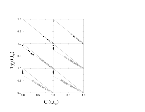
Figure 13: Movie plot for sample ${\cal H}_{A}$ of Sec. 4. Here we use $h=0.1$, $T=0.4$, and $t_{w}=10^{4}$. The different frames correspond to (from left to right and top to bottom): $\Delta t=2^{4}$, $2^{9}$, $2^{12}$, $2^{15}$, $2^{16}$, and $2^{17}$. Black and white circles refer, respectively, to type-I and type-II sites. Continuous lines correspond to ordinary FDT $\chi_{i}=(1-C_{i})/T$, while dotted ones are fits to a modified relation $\chi_{i}=(1-C_{i})/T_{\rm movie}$. We get $T_{\rm movie}=0.459$ (for $t=2^{12}$), $0.536$ ($t=2^{15}$), $0.564$ ($t=2^{16}$), $0.590$ ($t=2^{17}$).

In Fig. 13 we reproduce the correlation and response functions of all the spins of sample ${\cal H}_{A}$ in a movie plot. We fix $t_{w}=10^{4}$ and watch the single-spin correlation and response functions, as the system evolves, i.e. as $t$ grows. The behavior can be described as follows: $(i)$ for small $t$, all the points $(C_{i},\chi_{i})$ stay on the fluctuation dissipation line $T\chi_{i}=1-C_{i}$, type-I and type-II spins cannot be distinguished; $(ii)$ as $t$ grows, type-I spins reveal to be “faster” than type-II ones and move rapidly toward the $C=0$,$\chi=1$ corner; $(iii)$ just after this, type-II spins move out of the FDT relation, all together; $(iv)$ type-II keep evolving in the $C$-$\chi$ plane but, amazingly, they stay, at each time on a unique (moving) line passing through $C=1$, $\chi=0$.

On the same graphs, in Fig. 13, we show the results of a fit of the type

$$\chi_{i}(t,t_{w})=\frac{1}{T_{\rm movie}(t,t_{w})}[1-C_{i}(t,t_{w})]\,.$$ (4.7)

The fit works quite well: it allows to define a new effective temperature: the “movie” temperature $T_{\rm movie}(t,t_{w})$. The thermometrical interpretation of $T_{\rm movie}(t,t_{w})$ will be discussed in Sec. 8. $T_{\rm movie}(t,t_{w})$ increases with $t$ at fixed waiting time $t_{w}$. Notice the difference between this formula, and Eq. (3.14) which we argued to hold for coarsening systems. The organization of heterogeneous degrees of freedom in the $\chi$-$C$ plane is strongly dependent upon the nature of the physical system as a whole.

The cautious reader will notice a few discrepancies between the above description and the data in Fig. 13. Type-I spins reach the $(C=0,\chi=1)$ corner slightly after type-II ones move out of the FDT line. A careful check shows that this is a finite-$t_{w}$ artifact. Moreover, for large times, they stay slightly below the FDT line. This phenomenon has been discussed in Sec. 4.1.2 and proved to be a finite-$h_{0}$ effect.

Figure 14: On the left, the FD plot for seven different sites: $i=10$ ($+$), $11$ ($\circ$), $12$ (filled squares), $13$ ($\Box$), $16$ ($\times$), $17$ ($\ast$), $18$ ($\bullet$). On the right, a collapse plot of the same data, cf. Eq. (4.8). Here $T=0.3$, $h_{0}=0.1$, $t_{w}=10^{4}$, and we use $\overline{q}=0.94$.

Figure 15: Correlation between the theoretical prediction for the local EA parameters and the results of out-of-equilibrium simulations. On the left we show the data for sample ${\cal H}_{A}$ ($T=0.5$, $t_{w}=10^{3}$, and $h_{0}=0.1$), on the right for sample ${\cal H}_{B}$ ($T=0.4$, $t_{w}=10^{3}$, and $h_{0}=0.1$).

Figure 16: Distribution of the slopes of single-site OFDR’s for $T=0.4$. The vertical lines correspond to the theoretical prediction for the 1RSB parameter $m_{\rm th}$. On the left (right) we kept $h_{0}=0.05$ ($t_{w}=10^{4}$) fixed.

Let us now consider the local OFDR’s, and compare the dynamical results with the static 1RSB prediction (4.4). A preliminary check was given in Fig. 10. In Fig. 14, left frame, we reproduce the $\chi_{i}$ versus $C_{i}$ curves for 7 type-II sites. They are superimposed for short times (quasi-equilibrium regime) and spread at later times (aging regime), but remaining roughly parallel to each other. If the static prediction (4.4) holds, we can collapse the various $\chi_{i}[C_{i}]$ curves by properly rescaling $\chi_{i}$ and $C_{i}$. A particular form of rescaling, which is quite natural for coarsening systems, was used in Sec. 3.1.2, cf. Eqs. (3.13). It turns out that, in this case, a better collapse can be obtained by using the definition below:

$$C_{i}^{\rm res}=1-\frac{1-\overline{q}}{1-q_{\rm\scriptscriptstyle EA,th}^{(i)}}(1-C_{i})\,,\;\;\;\;\;\;\chi_{i}^{\rm res}=\frac{1-\overline{q}}{1-q_{\rm\scriptscriptstyle EA,th}^{(i)}}\chi_{i}\,,$$ (4.8)

where $\overline{q}$ is a reference overlap (which can be chosen freely). In Fig. 14, right frame, we plot $\chi_{i}^{\rm res}$ and $C_{i}^{\rm res}$ for the same 7 spins as before, computing the $q_{\rm\scriptscriptstyle EA,th}^{(i)}$ with the SP_T algorithm. Note that there is no fitting parameter in this scaling plot.

It can be interesting to have a more general look at the statics-dynamics relation. In order to make a comparison, we fitted the single-site $\chi_{i}$-versus-$C_{i}$ data to the theoretical prediction (4.4). The results for the two fitting parameters $q_{\rm\scriptscriptstyle EA}^{(i,{\rm fit})}$ and $m^{(i,{\rm fit})}$, are compared in Figs. 15, 16 with the outcome of the SP_T algorithm. Although several sources of error affect the determination of the EA parameters from dynamical data, the agreement is quite satisfying.

Figure 17: Movie plot for sample ${\cal H}_{B}$ ($T=0.4$, $h_{0}=0.1$): we show the position of all the degrees of freedom in the $\chi$-$C$ plane, for $t_{w}=10^{3}$ and $\Delta t=2^{16}$. The thin continuous lines are the FD plots for a few selected sites (in this case $\Delta t$ varies between $0$ and $2^{16}$). In the inset: the histogram of slopes of the FD curves in the out-of-equilibrium regime.

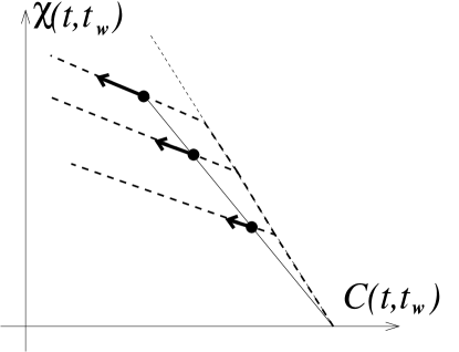
Figure 18: Qualitative picture of aging dynamics for discontinuous glasses. The black circles correspond to three different spins for a given pair of (large) times $(t,t_{w})$. Notice that, for intermediate times $\Delta t\sim t_{w}$ they stay on the same line passing through the point $(C=1,\chi=0)$. As $t$ grows, they move with parallel velocities (arrows). Along the time, each of them describes a different fluctuation-dissipation curve (dashed lines).

In the above paragraphs we stressed two properties of the aging dynamics of the model (4.1): the alignment in the movie plots, cf. Fig. 13 and Eq. (4.7), and the OFDR (4.4). Let us notice that these two properties are not compatible at all times $(t,t_{w})$. In fact we expect our model to verify the weak ergodicity-breaking condition $\lim_{t\to\infty}C_{i}(t,t_{w})=0$. Therefore, in this limit, the alignment (4.7) cannot be verified unless the $\chi_{i}$ become site-independent. On the other hand, this would invalidate the OFDR (4.4).

One plausible way-out to this contradiction is that Eq. (4.7) breaks down at large enough times. How this may happen is well illustrated by the numerical data concerning sample ${\cal H}_{B}$ shown in Fig. 17. It is quite clear that the simple law (4.7) no longer holds. Nevertheless, it remains a very good approximation for the sites with a large EA parameter $q_{\rm\scriptscriptstyle EA}^{(i)}\gtrsim 0.5$. Moreover, it seems that the points corresponding to different sites still lie on the same curve in the $\chi$-$C$ plane, although this curve is not a straight line as in Eq. (4.7). We shall further comment on this point in Sec. 7.

The general picture which holds at intermediate times (or large $q_{\rm\scriptscriptstyle EA}^{(i)}$’s) for discontinuous glasses is summarized in Fig. 18. This should be compared with Fig. 1, which refers to coarsening systems.

5 Continuous glasses

The Viana-Bray model [17] is a prototypical example of continuous spin glass. It is defined by the Hamiltonian

$$H(\sigma)=-\sum_{(ij)\in{\cal G}}J_{ij}\sigma_{i}\sigma_{j}\,,$$ (5.1)

where the graph ${\cal G}$ is constructed by randomly choosing $M$ among the $N(N-1)/2$ couples of spins, and the couplings $J_{ij}$ are independent identically distributed random variables. The average connectivity of the graph is given by $c=2M/(N-1)$. If we assume that the couplings distribution is even, the phase diagram of this model is quite simple [17, 43]. For $c<1$ the interaction graph does not percolate and the model stays in its paramagnetic phase at all finite temperatures. For $c>1$ the graph percolates and the giant component undergoes a paramagnetic-spin glass phase transition. The critical temperature is given by the solution of the equation $\mathbb{E}_{J}(\tanh\beta J)^{2}=1/c$. Below the critical temperature, a finite Edwards-Anderson parameter $q_{\rm\scriptscriptstyle EA}$ develops continuously from zero.

We considered three samples of this model: hereafter they will be denoted as ${\cal G}_{A}$, ${\cal G}_{B}$ and ${\cal G}_{C}$. The interaction graph and the signs of the interactions $J_{ij}$ were the same for ${\cal G}_{A}$ and ${\cal G}_{B}$: in particular we used $N=1000$ and $M=1999$, i.e. $c\approx 4$, and chosen the interaction signs to be $\pm 1$ with equal probabilities. The two samples differ only in the strength of the couplings. While in ${\cal G}_{A}$ we used $|J_{ij}|=1$, in ${\cal G}_{B}$ we took $|J_{ij}|=kJ_{0}$, where $k\in\{1,\dots,10\}$ with uniform probability distribution and $J_{0}=0.161164$. We made this choice in order to check the effects of degenerate coupling strengths on the aging dynamics. The sample ${\cal G}_{C}$ was instead much larger: we used $N=10000$, $M=20190$ (once again $c\approx 4$) and $J_{ij}=\pm 1$ with equal probabilities. The critical temperatures for $c=4$ and the two coupling distributions used here are $T_{c}\approx 1.8204789$ (for ${\cal G}_{A}$ and ${\cal G}_{C}$) and $1.6717415$ (${\cal G}_{B}$).

The glassy phase of the VB model is thought to be characterized by FRSB. Nevertheless we can use the SP_T algorithm to compute a one-step approximation to the local overlaps and the local OFDR’s. Of course, such an approximation will have the simple two time-sectors form, see Eq. (4.4), instead of the expected infinite-time-sectors behavior. However the situation is not that simple because of two problems:

• We expect, in analogy with the Sherrington-Kirkpatrick model [29], the dynamics of this model to reach the equilibrium free-energy in the long time limit. It is not clear whether a better approximation to the correct OFDR is obtained by using the threshold value $m_{\rm th}$ or the ground-state value $m_{\rm gs}$ of the 1RSB parameter.

• The SP_T algorithm does not converge. After a fast transient the probability distributions of local fields oscillate indefinitely. This is, plausibly, a trace of FRSB.

The first problem does not cause great trouble because the two determinations of $m$ are, generally speaking, quite close. On the other hand, we elaborated two different way-out to the second one: $(i)$ To force the local field distributions to be symmetric (which can be expected to be true on physical grounds): this assures convergence. $(ii)$ To average the local EA parameters over sufficiently many iterations of the algorithm.

While the approach $(i)$ seems physically more sound, it underestimates grossly the $q^{(i)}_{\rm EA}$’s. The approach $(ii)$, which will be adopted in our analysis, gives much more reasonable results. Notice that the authors of Refs.[22, 44] followed the same route. In their calculation, they faced no problem of convergence. In fact they required convergence in distribution, while we require convergence site-by-site.

5.1 Numerical results

Most of our simulations were run at temperature $T=0.5$, and with $h_{0}=0.1$. We used waiting times $t_{w}=10^{2}$, $10^{3}$, $10^{4}$, and, respectively $\Delta t_{\rm MAX}=2^{14}$, $2^{16}$, $2^{18}$. In the Table below we summarize the statistics used in each case.

	$t_{w}=10^{2}$	$t_{w}=10^{3}$	$t_{w}=10^{4}$
${\cal G}_{A}$	$10^{6}$	$4\cdot 10^{5}$	$5.5\cdot 10^{5}$
${\cal G}_{B}$	$6\cdot 10^{5}$	$1.5\cdot 10^{6}$	$\ast$
${\cal G}_{C}$	$6\cdot 10^{5}$	$\ast$	$\ast$

Moreover we simulated $N_{\rm stat}=4.2\cdot 10^{5}$ Metropolis trajectories at temperature $T=0.4$ on sample ${\cal G}_{A}$ with $t_{w}=10^{4}$ and $\Delta t_{\rm MAX}=2^{18}$.

Figure 19: Single-spin correlation and response functions for the sample ${\cal G}_{A}$ (VB model) for $T=0.5$, $h_{0}=0.1$, and $t_{w}=10^{4}$. The continuous line and full circle refer to the global correlation and response.

Figure 20: Single-spin correlation and response functions: here we compare the results obtained on samples ${\cal G}_{A}$ ($\circ$) and ${\cal G}_{C}$ ($\bullet$) which are of different sizes.

In Fig. 19 we show the movie plot of sample ${\cal G}_{A}$ for $t_{w}=10^{4}$. As in the previous Sections, the local correlation and response functions are strongly heterogeneous: the global two-times functions give just a rough idea of the dynamics of the system. Moreover all the points quit the FDT line on the same time scale in the aging limit (cf. Sec. 4.1.3). However, their behavior in the aging regime does not fit any of the alignment patterns we singled-out in the case of coarsening systems, cf. Eq. (3.14) and Fig. 1, or discontinuous glasses, cf. Eq. (4.7) and Fig. 18. We repeated the same type of analysis for the numerical data obtained on sample ${\cal G}_{C}$. In this case, see Fig. 20, the points corresponding to local correlation and response functions are much less spread in the $\chi$-$C$ plane. Therefore our simulations are quite inconclusive on the possibility of defining a “movie” temperature as in Eq. (4.7). To settle the question, simulations on larger samples are probably necessary.

Figure 21: FD plot for a few selected sites of sample ${\cal G}_{A}$ ($T=0.5$, $h_{0}=0.1$). Notice the completely different behaviors of the sites in the two frames. The sites in the left frame, with connectivity $1$ (site $111$) and $3$ (site $164$), look like a “glassy” system. The ones on the right, with connectivity $4$ (site $103$) and $2$ (site $114$), look like a “coarsening” system.

Numerical results on sample ${\cal G}_{A}$ are also deceiving for what concerns local OFDR’s, cf. Fig. 21. It seems that the local FD plots depend strongly upon the waiting time and the particular site. Moreover the slopes of this plots (for a given couple $(t_{w},\Delta t)$) change from site to site.

Figure 22: Distributions of slopes of the local FD plots in the aging regime. The two curves refer to sample ${\cal G}_{A}$ ($\circ$) and ${\cal G}_{C}$ ($\bullet$), which are of different sizes.

These effects are much smaller in sample ${\cal G}_{C}$. In Fig. 22 we consider the distribution of slopes of local FD plots for samples ${\cal G}_{A}$ and ${\cal G}_{C}$. We computed the slopes by fitting the aging part of the plot to the one-step form (4.4).

Figure 23: Local EA parameters on sample ${\cal G}_{C}$. Numerical results, obtained by fitting the aging part of the FD plots, are compared with the outcome of the SP_T algorithm.

By the same fitting procedure we extracted the local EA parameters. The comparison with the predictions of the SP_T algorithm, cf. Fig. 23 is quite satisfying. Notice that, both in analyzing the numerical data and in using the SP_T algorithm, we are adopting a 1RSB approximation, cf. Eq. (4.4), to the real OFDR. The slopes considered in Fig. 22 should therefore be understood as average slopes in the aging regime. We expect the systematic error induced by this approximation to be small.

The arguments of Ref. [45] imply that the slopes (effective temperatures) of the OFDR’s for different degrees of freedom should be identical. This conclusion is valid only in the aging window $1\ll t_{w},\Delta t\ll t_{\rm erg}(N)$. Our numerical data, cf. Fig. 22, suggest a clear trend confirming this expectation. Nevertheless, they show large finite-size effects due, arguably, to a mild divergence of $t_{\rm erg}(N)$ with $N$: the smaller ($N=10^{3}$) samples begin to equilibrate during the simulations. This is quite different from what happens with discontinuous glasses, cf. Sec. 4. In that case, we did not detect any evidence of equilibration even in sample ${\cal H}_{A}$ ($N=10^{2}$). A better understanding of the scaling of $t_{\rm erg}(N)$ in different classes of models would be welcome.

6 Weakly interacting spins

We lack of analytical tools for studying the dynamics of diluted mean-field spin glasses (for some recent work see Refs. [46, 47, 48, 49]). This makes somehow ambiguous the interpretation of many numerical results. For instance, the identity of effective temperatures for different spins, although consistent with our data, see Figs. 16 and 22, could still be questioned. This would contradict the general arguments of Refs. [45, 50]. Even more puzzling is the definition of a “movie” temperature along the lines of Eq. (4.7). Such a definition seems to be consistent only in some particular models and time-regimes. In this Section we want to point out a simple perturbative calculation which supports the identity of single-spin effective temperatures, in agreement with the standard wisdom. Moreover it give some intuition on the range of validity of the definition (4.7).

Let us consider a generic diluted mean-field spin glass with $k$-spin interactions:

$$H(\sigma)=-\sum_{\underline{\alpha}\in{\cal H}}J_{\underline{\alpha}}\sigma_{\alpha_{1}}\cdot\dots\cdot\sigma_{\alpha_{k}}\,.$$ (6.1)

Here $\underline{\alpha}=\{\alpha_{1},\dots,\alpha_{k}\}$ is a $k$-uple of interacting spins, and ${\cal H}$ is a $k$-hypergraph, i.e. a set of $M$ such $k$-uples.

Let us focus on a particular site, for instance $i=0$, and assume that it is weakly coupled to its neighbors. It is quite natural to think that its response and correlation functions can be related to the response and correlation functions of the neighbors. To the lowest order this relation reads:

$$C_{0}^{\rm ag}(t,t_{w}) = \sum_{\underline{\alpha}\ni 0}(\tanh\beta J_{\underline{\alpha}})^{2}\prod_{i\in\underline{\alpha}\backslash 0}C_{i}^{\rm ag}(t,t_{w})+O(\beta^{4}J^{4})\,,$$ (6.2)

$$R_{0}^{\rm ag}(t,t_{w}) = \sum_{\underline{\alpha}\ni 0}(\tanh\beta J_{\underline{\alpha}})^{2}\sum_{i\in\underline{\alpha}\backslash 0}R_{i}^{\rm ag}(t,t_{w})\prod_{j\in\underline{\alpha}\backslash\{0,i\}}C_{j}^{\rm ag}(t,t_{w})+O(\beta^{4}J^{4})\,.$$ (6.3)

We shall not give here the details of the derivation. The basic idea is to use an appropriate dynamic generalization of the cavity method [51, 52]. As for static calculations [21], this approach gives access to single-site quantities for a given disorder realization. Notice that Eq. (6.2) can be easily obtained by assuming that the spin $\sigma_{0}$ does not react on its neighbors. This is not the case for Eq. (6.3).

Equation (6.2) implies a relation between local Edwards-Anderson parameters:

$$q_{\rm\scriptscriptstyle EA}^{(0)} = \sum_{\underline{\alpha}\ni 0}(\tanh\beta J_{\underline{\alpha}})^{2}\prod_{i\in\underline{\alpha}\backslash 0}q_{\rm\scriptscriptstyle EA}^{(i)}+O(\beta^{4}J^{4})\,.$$ (6.4)

In the $k=2$ (Viana-Bray) case, we can derive from Eq. (6.3) a simple relation between the integrated responses:

$$1-T\chi_{0}^{\rm ag}(t,t_{w}) = \sum_{i\in\partial 0}(\tanh\beta J_{0i})^{2}[1-T\chi_{i}^{\rm ag}(t,t_{w})]+O(\beta^{4}J^{4})\,,$$ (6.5)

where $\partial i_{0}$ denote the set of neighbors of the spin $i_{0}$. In the general ($k>2$) case Eq. (6.3) cannot be integrated without further assumptions.

Figure 24: FD plots for a few weakly-interacting spins: numerical results ($\bullet$) and outcomes of the perturbative formulae (6.2) and (6.5) ($\circ$). We consider connectivity-1 sites on the left, and connectivity-2 sites on the right.

We checked the above relations on our numerical data for the Viana-Bray model. Sample ${\cal G}_{B}$ is particularly suited for this task, since we can choose spins whose interactions have a varying strength. In Fig. 24, we consider a few spins with connectivity one and two, and compare their correlation and response functions with the outcome of Eqs. (6.2) and (6.5). Of course, the perturbative formulae are well verified only for small couplings. For connectivity-2 sites we have plotted in Fig. 24 only those with coupling of the same strenght, since spins with 2 couplings of very different strengths behave very similarly to connectivity-1 spins.

Let us now discuss some implications of Eqs. (6.2), (6.3). If we define the fluctuation-dissipation ratio as $X_{i}(t,t_{w})\equiv TR_{i}^{\rm ag}(t,t_{w})/\partial_{t_{w}}C_{i}^{\rm ag}(t,t_{w})$, we get:

$$X_{0}(t,t_{w})\approx\frac{\sum_{\underline{\alpha}\ni 0}\sum_{i\in\underline{\alpha}\backslash 0}W_{\underline{\alpha},i}(t,t_{w})X_{i}(t,t_{w})}{\sum_{\underline{\alpha}\ni 0}\sum_{i\in\underline{\alpha}\backslash 0}W_{\underline{\alpha},i}(t,t_{w})}\,,$$ (6.6)

where

$$W_{\underline{\alpha},i}(t,t_{w})\equiv(\tanh\beta J_{\underline{\alpha}})^{2}\partial_{t_{w}}C_{i}(t,t_{w})\prod_{j\in\underline{\alpha}\backslash\{i,0\}}C_{j}(t,t_{w})$$ (6.7)

are positive weights. Therefore, at the lowest order in perturbation theory, the effective temperature of the spin $\sigma_{0}$ is a weighted average of the effective temperatures of its neighbors. Let us suppose that this conclusion remains qualitatively true beyond perturbation theory. It follows that $X_{i}(t,t_{w})=X(t,t_{w})$ is independent of the site $i$. In fact, if the $X_{i}(t,t_{w})$ were site-dependent we could just consider a site $i_{*}$ such that $X_{i_{*}}(t,t_{w})$ is a relative maximum and show that Eq. (6.6) cannot hold on such a site. With a suggestive rephrasing we may say that effective temperatures must diffuse until they becomes site-independent.

Moreover, Eqs. (6.2) and (6.3) can be used to construct examples of weakly interacting spins which violate the alignment in the $\chi$-$C$ plane which we encountered for discontinuous glasses, cf. Eq. (4.7) and Fig. 13. The simplest of such examples is obtained by considering the Viana-Bray ($k=2$) case, and assuming that the site 0 has just one neighbor. In this case it is immediate to show that

$$\frac{C_{0}^{\rm ag}(t,t_{w})}{1-T\chi_{0}(t,t_{w})}\approx\frac{C_{i}^{\rm ag}(t,t_{w})}{1-T\chi_{i}(t,t_{w})}\,,$$ (6.8)

i.e. weakly interacting spins have the tendency to align as in coarsening systems. The reader can easily construct analogous examples for $k>2$ models. This suggests that the “movie” temperature (4.7) is well defined uniquely for strongly interacting and glassy systems, or, in other words, for slow-evolving sites with a $q_{\rm\scriptscriptstyle EA}^{(i)}$ close to one.

7 Discussion

In the last two Sections we shall discuss the general properties of single-spin correlation and response functions which emerge from the numerics. We will give an overview of such properties in the present Section, and precise the thermometric interpretation of some of them in the next one.

We shall focus on two-times correlation and response functions $C_{i}(t,t_{w})$ and $R_{i}(t,t_{w})$ (see [47] for a preliminary discussion of multi-time functions) and distinguish two types of facts: $(i)$ their scaling behavior in the large time limit; $(ii)$ the fluctuation-dissipation relations which connect correlation and response.

7.1 Time scaling

Following Refs. [29, 30], we assume monotonicity of the two-times functions: $\partial_{t}C_{i}(t,t_{w})$, $\partial_{t}R_{i}(t,t_{w})\leq 0$, and $\partial_{t_{w}}C_{i}(t,t_{w})$, $\partial_{t_{w}}R_{i}(t,t_{w})\geq 0$. Moreover we consider a weak-ergodicity breaking situation: $C_{i}(t,t_{w}),\,R_{i}(t,t_{w})\to 0$ as $t\to\infty$ for any fixed $t_{w}$. All these properties are well realized within our models.

It is quite natural to assume that, for pair of sites $i$ and $j$ there exist two continuous functions $f_{ij}$ and $f_{ji}$ such that

$$C_{i}(t,t_{w})=f_{ij}[C_{j}(t,t_{w})]\,,\;\;\;\;C_{j}(t,t_{w})=f_{ji}[C_{i}(t,t_{w})]\,,$$ (7.1)

in the $t,t_{w}\to\infty$ limit. Notice that we can always write

$$C_{i}(t,t_{w})=f_{ij}[C_{j}(t,t_{w}),t]\,.$$ (7.2)

We are therefore assuming that the functions $f_{ij}[C,t]$ admit a limit as $t\to\infty$ and that the limit is continuous. Since $f_{ij}[C,t]$ is smooth and $\partial_{C}f_{ij}[C,t]\geq 0$, if the limit exists it must be a continuous, non-decreasing function of $C$. Since Eq. (7.1) implies that both $f_{ij}$ and $f_{ji}$ are invertible (indeed $f_{ij}\circ f_{ji}=1$, see below) they must be strictly increasing.

Without any further specification, the property (7.1) is trivially false. Consider the example of type-I (paramagnetic) spins in the 3-spin model studied in Sec. 4. If $i$ is type-I, and $j$ is type-II, $C_{i}(t,t_{w})\to 0$ in the aging regime, while $C_{j}(t,t_{w})$ remain non-trivial: $f_{ij}[\cdot]$ cannot be inverted. Another example, would be that of a Viana-Bray model, cf. Sec. 5, such that the interactions graph has two disconnected components.

However, both these counter-examples are somehow “pathological”. We can precise this intuition by noticing that Eq. (7.1) defines an equivalence relation (in mathematical sense) between the sites $i$ and $j$. Therefore the physical system breaks up into dynamically connected components which are the equivalence classes of this relation. Type-I and type-II spins in the 3-spin model of Sec. 4 are two examples of dynamically connected components. Hereafter we shall restrict our attention to a single dynamically connected component. Physically, structural rearrangements occurs coherently within such a component.

Clearly the transition functions $\{f_{ij}\}$ have the following two properties: $(i)$ $f_{ji}=f^{-1}_{ij}$, and $(ii)$ $f_{ij}=f_{ik}\circ f_{kj}$. This implies that they can be written in the form $f_{ij}=f_{i}^{-1}\circ f_{j}$ (the proof consists in taking a reference spin $k=0$ and writing $f_{ij}=f_{i0}\circ f_{0j}=f_{0i}^{-1}\circ f_{0j}$). Of course the functions $f_{i}$ are not unique: in particular they can be modified by a global reparametrization $f_{i}\to g\circ f_{i}$.

Although very simple, the hypothesis (7.1) has some important consequences. Suppose that $C_{j}(t,t_{w})$ has $p$ discrete correlation scales (in the sense of Refs. [29, 30]), characterized by $q^{(j)}_{\alpha+1}<C_{j}(t,t_{w})\leq q^{(j)}_{\alpha}$, for $\alpha=1,\dots,p$. Within a scale we have

$$C_{j}(t,t_{w})\approx{\cal C}^{(\alpha)}_{j}(h^{(j)}_{\alpha}(t)/h^{(j)}_{\alpha}(t_{w}))\,.$$ (7.3)

where $h^{(j)}_{\alpha}(t)$ is a monotonously increasing time-scaling function. Two times $t$ and $t_{w}$ belong to the same time sector if $1<h^{(j)}_{\alpha}(t)/h^{(j)}_{\alpha}(t_{w})<\infty$.

Applying the transition function $f_{ij}$ to the above equation, one can prove that, for each scale $\alpha$ of the site $j$, there exists a correlation scale for the site $i$, with $q^{(i)}_{\alpha+1}<C_{i}(t,t_{w})\leq q^{(i)}_{\alpha}$ and $q^{(i)}_{\cdot}=f_{ij}[q^{(j)}_{\cdot}]$. Moreover $h^{(i)}_{\alpha}(t)=h^{(j)}_{\alpha}(t)\equiv h_{\alpha}(t)$ (up to an irrelevant multiplicative constant) and

$${\cal C}^{(\alpha)}_{i}=f_{ij}\circ{\cal C}^{(\alpha)}_{j}\,.$$ (7.4)

In summary there is a one-to-one correspondence between the correlation scales of any two sites. Notice that this is a necessary hypothesis if we want the connection between statics and dynamics [27, 28] to be satisfied both at the level of global and local (single-spin) observables. A spectacular demonstration of the correspondence of correlation scales on different sites is given by our movie plots, cf. Figs. 5, 13 and 19. In particular such correspondence implies that all the $(\chi_{i},C_{i})$ points leave the FDT line at once.

Equation (7.1) can be rephrased by saying that the behavior of one spin “determines” the behavior of the whole system. This is compatible with the locality of the underlying dynamics because: $(i)$ “determines” has to be understood in average sense; $(ii)$ the relation (7.1) is not true but in the aging limit.

7.2 Fluctuation-dissipation relations

On general grounds, we expect single-spin quantities to to satisfy site-dependent OFDR’s of the type (2.3). In integrated form we obtain, for large times $t,t_{w}$, the relation $\chi_{i}(t,t_{w})=\chi_{i}[C_{i}(t,t_{w})]$. We think that we accumulated convincing numerical evidence in this direction as far as the models of Secs. 3 (coarsening) and 4 (discontinuous spin glass) are considered. The situation is more ambiguous (and probably very hard to settle numerically) for the Viana-Bray model of Sec. 5.

Fluctuation-dissipation relations on different sites are not unrelated: we expect [45] to be able to define a site-independent effective temperature as follows

$$\chi_{i}^{\prime}[C_{i}(t,t_{w})]=\chi_{j}^{\prime}[C_{j}(t,t_{w})]\equiv-\frac{1}{T_{\rm eff}(t,t_{w})}\,.$$ (7.5)

In terms of transition functions, we get $\chi_{i}^{\prime}[C_{i}]=\chi_{j}^{\prime}[C_{j}]$ when $C_{i}=f_{ij}[C_{j}]$. As before, the numerics support this identity both for coarsening systems, cf. Sec. 3, and discontinuous glasses, cf. Sec. 4. For continuous glasses, cf. Sec. 5, the situation is less definite. In Sec. 6 we presented a perturbative calculation which support Eq. (7.5) also in this case.

A suggestive approach [50] for justifying (7.5) consists in regarding $T_{\rm eff}(t,t_{w})$ as the temperature measured by a thermometer coupled to a particular observable of the system. It is quite natural to think that the result of this measure should not depend upon the observable. In aging systems with more than just one time sector, this approach is not consistent unless the following identity holds:

$$\frac{\chi_{i}(t,t_{w})}{1-C_{i}(t,t_{w})}=\frac{\chi_{j}(t,t_{w})}{1-C_{j}(t,t_{w})}\equiv\frac{1}{T_{\rm movie}(t,t_{w})}\,.$$ (7.6)

Proving this conclusion will be the object of the next Section. The new effective temperature $T_{\rm movie}(t,t_{w})$ is in fact the one measured by a particular class of thermometers which we shall denote as “sharp”. It is a weighted average of the effective temperatures (in the sense of (7.5)) corresponding to different time sectors.

Let us notice that Eq. (7.6) is remarkably well verified in our discontinuous spin-glass model, cf. Fig. 13, although it breaks down for $(t/t_{w})\gg 1$. In Sec. 3 we demonstrated that it does not hold for coarsening systems, and in fact a different relation is true in this case, cf. Eq. (3.14). Finally, we were not able to reach any definite conclusion for the Viana-Bray model of Sec. 5.

8 Thermometric interpretation

One of the most striking (and unexpected) observations we made on our numerical results is summarized in Eq. (7.6). In this Section we shall try to connect this empiric observation to thermometric considerations. This type of approach was pioneered in Ref. [50] with the aim of interpreting the OFDR in terms of effective temperatures. Here we will show that, in a system with more than a single time scale, this interpretation is well founded if and only if the “movie” temperature (7.6) can be defined. In order to obtain this result, we shall carefully reconsider the arguments of Refs. [50, 53, 54].

According to Ref. [50], the temperature of a out-of-equilibrium system can be measured by weakly coupling it to a “thermometer”, i.e. to a physical device which can be equilibrated at a tunable temperature $T_{\rm th}=1/\beta_{\rm th}$. The temperature of the system is defined as the value of $T_{\rm th}$ such that the heat flow between it and the thermometer vanishes. The details of the thermometer are immaterial in the weak-coupling limit. What matters are the correlation and response functions of the thermometer $C_{\rm th}(t,t_{w})=C_{\rm th}(t-t_{w})$ and $R_{\rm th}(t,t_{w})=R_{\rm th}(t-t_{w})$, which are assumed to satisfy FDT: $R_{\rm th}(\tau)=-\beta_{\rm th}\partial_{\tau}C_{\rm th}(\tau)$.

In the spirit of our work, we shall couple the thermometer to a single spin variable $\sigma_{i}$ between times $0$ and $t$, and average over many thermal histories. The measured temperature $\beta_{\rm th}$ is given by [50, 53]

$$\beta_{\rm th}\int_{0}^{t}\!\!dt_{w}\,\,R_{\rm th}(t-t_{w})\partial_{t_{w}}C_{i}(t,t_{w})=\int_{0}^{t}\!\!dt_{w}\,\,R_{\rm th}(t-t_{w})(-\chi_{i}^{\prime}[C_{i}(t,t_{w})])\partial_{t_{w}}C_{i}(t,t_{w})\,,$$ (8.1)

where we assumed the general OFDR (2.3) in its integrated form: $\chi_{i}(t,t_{w})=\chi_{i}[C_{i}(t,t_{w})]$, and denoted by a prime the derivative of $\chi_{i}[\cdot]$ with respect to its argument. Notice that a priori the measured temperature depends upon $i$ and $t$, for a given thermometer.

It is convenient to change variables from $t_{w}$ to $q\equiv C_{i}(t,t_{w})$. This relation can be inverted by defining the time scale $\tau_{i}(t;q)$ as follows:

$$C_{i}(t,t-\tau_{i}(t;q))=q\,.$$ (8.2)

Using these definitions in Eq. (8.1), we get

$$\beta_{\rm th}\int_{q_{\rm min}}^{1}\!\!\!dq\,\,R_{\rm th}(\tau_{i}(t;q))=\int_{q_{\rm min}}^{1}\!\!\!dq\,\,R_{\rm th}(\tau_{i}(t;q))(-\chi_{i}^{\prime}[q])\,,$$ (8.3)

where $q_{\rm min}\equiv C_{i}(t,0)$. As $t\to\infty$, we have $q_{\rm min}\to 0$. In the same limit $\tau_{i}(t;q)\to\tau^{\rm eq}_{i}(q)$ if $q>q_{\rm\scriptscriptstyle EA}^{(i)}$, while $\tau_{i}(t;q)\to\infty$ if $q<q_{\rm\scriptscriptstyle EA}^{(i)}$.

In order to measure temperatures on long time scales, we need a thermometer with an adjustable time scale. Mathematically speaking, we take $R_{\rm th}(\tau)=\widetilde{R}_{\rm th}(\tau/\tau_{\rm th})$, and use $\tau_{\rm th}$ to select the time scale. The precise form of $\widetilde{R}_{\rm th}(x)$ is not very important. We shall assume that $\widetilde{R}_{\rm th}(x)\approx 1$ for $x\ll 1$ and $\widetilde{R}_{\rm th}(x)\approx 0$ for $x\gg 1$. A simple example is $\widetilde{R}_{\rm th}(x)=\theta(x)\,e^{-x}$. Some of the relations we will derive simplify if $\widetilde{R}_{\rm th}(x)\approx\theta(x)\theta(x_{*}-x)$. We will call such a thermometer “sharp”.

We have two type of choices for the thermometer time scale $\tau_{\rm th}$:

1. We may take a “fast” thermometer, whose relaxation is much faster than the structural rearrangements of the system. Equivalently: we look at our thermometer after a time $t\gg\tau_{\rm th}$. Mathematically this corresponds to taking the limit $t\to\infty$ with $\tau_{\rm th}$ fixed. The result of such a measure is (for large times $t$) the bath temperature.

2. We may use a “slow” thermometer, with a relaxation time which is of the same order of the time needed for a structural change in the system. This corresponds to taking the limits $t\to\infty$, $\tau_{\rm th}\to\infty$ at the same time. If the system ages, the outcome of such a measure will depend upon the precise way these limits are taken.

Let us consider separately the two cases.

8.1 “Fast” thermometer

In this case we have, as $t\to\infty$,

$$R_{\rm th}(\tau_{i}(t;q))\to\left\{\begin{array}[]{cl}F_{i}(q)=\widetilde{R}_{\rm th}(\tau_{i}^{\rm eq}(q)/\tau_{\rm th})&\mbox{for $q>q_{\rm\scriptscriptstyle EA}^{(i)}$,}\\ 0&\mbox{for $q<q_{\rm\scriptscriptstyle EA}^{(i)}$,}\end{array}\right.$$ (8.6)

with $F_{i}(q_{\rm\scriptscriptstyle EA}^{(i)})=0$ and $F_{i}(1)=1$. Inserting into Eq. (8.3) we get

$$\beta_{\rm th}\int_{q_{\rm\scriptscriptstyle EA}^{(i)}}^{1}\!\!dq\,F_{i}(q)=\int_{q_{\rm\scriptscriptstyle EA}^{(i)}}^{1}\!\!dq\,F_{i}(q)(-\chi_{i}^{\prime}[q])\,.$$ (8.7)

Assuming that in the “quasi-equilibrium” time sector (i.e. for $C_{i}(t,t_{w})>q_{\rm\scriptscriptstyle EA}^{(i)}$) the system satisfies FDT, we can use $\chi_{i}^{\prime}[q]=-\beta$, which yields $\beta_{\rm th}=\beta$, as expected.

8.2 “Slow” thermometer

Here we shall assume that the system has $p$ discrete correlation scales in the aging regime [30]. The generalization to a continuous set of correlation scales is straightforward. To each scale $\alpha\in\{1,\dots,p\}$ we associates a time-scaling function $h_{\alpha}(t)$. As discussed in Sec. 7, $h_{\alpha}(t)$ is site-independent.

In order to probe the correlation scale $\alpha$, we tune the thermometer time scale with the function $\tau_{{\rm th},A}(t)$. This function is defined by imposing

$$\frac{h_{\alpha}(t)}{h_{\alpha}(t-\tau_{{\rm th},A}(t))}=A\,,$$ (8.8)

for some fixed number $A>1$.

Within the scale $\alpha$, we have $q_{\alpha+1}^{(i)}<C_{i}(t,t^{\prime})<q_{\alpha}^{(i)}$. It is easy to show that

$$\lim_{t\to\infty}R_{\rm th}(\tau_{i}(t;q)/\tau_{{\rm th},A}(t))=F_{i,\alpha}(q)\,,$$ (8.9)

with $F_{i,\alpha}(q)=0$ for $q<q_{\alpha+1}^{(i)}$, $F_{i,\alpha}(q)=1$ for $q>q_{\alpha}^{(i)}$ and $F_{i,\alpha}(q)$ increasing in $(q_{\alpha+1}^{(i)},q_{\alpha}^{(i)})$. Integrating by parts Eq. (8.3), we get

$$\beta^{(i)}_{\rm th}\int_{0}^{1}\!dq\,F_{i,\alpha}^{\prime}(q)(1-q)=\int_{0}^{1}\!dq\,F_{i,\alpha}^{\prime}(q)\,\chi_{i}(q)\,,$$ (8.10)

which is our final expression for the temperature measured on the spin $i$ (here we emphasized the dependence of $\beta_{\rm th}$ upon the site).

Notice that the support of $F_{i,\alpha}^{\prime}(q)$ is contained in the interval $(q_{\alpha+1}^{(i)},q_{\alpha}^{(i)})$. The expression (8.10) simplifies in two cases: $(i)$ if the $\alpha$-th correlation scale is “small” $q_{\alpha+1}^{(i)}\approx q_{\alpha}^{(i)}\approx q^{(i)}_{*}$ (and, in particular, when there is a continuous set of scales); $(ii)$ if the thermometer is “sharp” in the sense defined at the beginning of this Section, and, therefore, $F_{i,\alpha}^{\prime}(q)$ is strongly peaked around some $q^{(i)}_{*}$. In both cases we have

$$\beta^{(i)}_{\rm th}\approx\frac{\chi_{i}(q^{(i)}_{*})}{1-q^{(i)}_{*}}\,.$$ (8.11)

Let us now imagine to couple two copies of the same thermometer to two different sites $i$ and $j$. We shall measure two temperatures $\beta^{(i)}_{\rm th}\approx\chi_{i}(q^{(i)}_{*})/(1-q^{(i)}_{*})$ and $\beta^{(j)}_{\rm th}\approx\chi_{j}(q^{(j)}_{*})/(1-q^{(j)}_{*})$, with $q^{(i)}_{*}=f_{ij}(q^{(j)}_{*})$. These two temperatures coincide, $\beta^{(i)}_{\rm th}\approx\beta^{(j)}_{\rm th}$, only if Eq. (7.6) is satisfied.

The conclusion of the arguments presented so far is that the condition (7.6) is necessary if we want a given thermometer to measure the same temperature on any two spins of the system. Moreover this condition is sufficient for the special class of “sharp” thermometers. In the last part of this Section we will show that the condition (7.6) is indeed sufficient for any thermometer, once (7.5) is assumed.

8.3 Thermometric equivalence of different sites

We want to prove that Eqs. (7.6) and (7.5) imply the identity of thermometric temperatures on the sites $i$ and $j$ for any given thermometer. Let us stress that the measured temperature may, eventually, depend upon the thermometer. The essential ingredient for the “small intropy production” scenario of Ref. [56] to be applicable, is that the result should not depend upon the site.

Notice that from the definition (8.2), it follows that the time scales defined on different sites are related as follows

$$\tau_{i}(t;f_{ij}(q))=\tau_{j}(t;q)\,,$$ (8.12)

whence we easily derive the identity $F_{i,\alpha}(f_{ij}(q))=F_{j,\alpha}(q)$. By the change of variables $q\to f_{ij}(q)$ we get, from Eq. (8.10)

$$\beta^{(i)}_{\rm th}\int_{q_{\alpha+1}^{(j)}}^{q_{\alpha}^{(j)}}\!dq\,\,F_{j,\alpha}^{\prime}(q)(1-f_{ij}(q))=\int_{q_{\alpha+1}^{(j)}}^{q_{\alpha}^{(j)}}\!dq\,\,F_{j,\alpha}^{\prime}(q)\,\chi_{i}(f_{ij}(q))\,,$$ (8.13)

where we specified the range of $q$ such that $F_{j,\alpha}^{\prime}(q)$ is (possibly) nonzero. If use Eq. (7.6) to connect the responses on different sites, we obtain

$$\beta^{(i)}_{\rm th}\int_{q_{\alpha+1}^{(j)}}^{q_{\alpha}^{(j)}}\!dq\,\,F_{j,\alpha}^{\prime}(q)(1-q)\left[\frac{1-f_{ij}(q)}{1-q}\right]=\int_{q_{\alpha+1}^{(j)}}^{q_{\alpha}^{(j)}}\!dq\,\,F_{j,\alpha}^{\prime}(q)\,\chi_{j}(q)\left[\frac{1-f_{ij}(q)}{1-q}\right]\,.$$ (8.14)

The factors $(1-f_{ij}(q))/(1-q)$ prevent us from concluding that $\beta^{(i)}_{\rm th}=\beta^{(j)}_{\rm th}$ with no further assumption. Let us assume Eq. (7.5), and that $\chi_{i}^{\prime}[q]$ stays constant for $q_{\alpha+1}^{(i)}<q<q_{\alpha}^{(i)}$. It follows that, within the scale $\alpha$, $f_{ij}(q)=1-f^{0}_{\alpha,ij}(1-q)$, $f^{0}_{\alpha,ij}$ being a constant. This implies $\beta^{(i)}_{\rm th}=\beta^{(j)}_{\rm th}$ for any thermometer.

Acnowledgements

This work received financial support from the ESF programme SPHINX and the EEC network DYGLAGEMEM.

Appendix A Large-$n$ calculations

In this Appendix we sketch the large-$n$ calculations whose results were presented in Sec. 3.1.1.

A.1 Statics

The trick for solving the periodic model of Sec. 3.1.1 is quite standard [58]. We define the $n\cdot V$-components vector $\mbox{\boldmath$\psi$}_{x}$ which contains $n$ components for each type of spin:

$$\psi^{a,u}_{x}=\phi^{a}_{x\cdot l+u}\,\,,\;\;u\in\Lambda\,,\,\,x\in{\mathbb{Z}}^{d}\,,$$ (A.1)

where $x\cdot l=\sum_{\mu=1}^{d}x_{\mu}l_{\mu}$ and $\Lambda$ is the elementary cell. In this basis the Hamiltonian reads

$$H(\mbox{\boldmath$\psi$})=-\sum_{x,\mu}\mbox{\boldmath$\psi$}_{x}\cdot\hat{\mathbb{K}}^{(\mu)}\mbox{\boldmath$\psi$}_{x+\mu}-\frac{1}{2}\sum_{x}\mbox{\boldmath$\psi$}_{x}\cdot\hat{\mathbb{L}}\mbox{\boldmath$\psi$}_{x}\,,$$ (A.2)

where $\hat{\mathbb{K}}_{au,bv}^{(\mu)}=\delta_{ab}{\mathbb{K}}_{u,v}^{(\mu)}$, $\hat{\mathbb{L}}_{au,bv}=\delta_{ab}{\mathbb{L}}_{u,v}$ and ${\mathbb{K}}_{u,v}=J_{u,\hat{\mu}l_{\mu}+v}$, ${\mathbb{L}}_{u,v}=J_{u,v}$.

The equilibrium correlation functions are computed by standard methods:

$$\langle\psi_{x}^{a,u}\rangle = \delta^{a,1}M_{u}\,,$$ (A.3)

$$\langle\psi_{x}^{a,u}\psi_{y}^{b,v}\rangle_{c} = T\int_{BZ}\!\frac{dp}{(2\pi)^{d}}\,[{\mathbb{M}}^{-1}_{*}(p)]_{u,v}\,e^{ip(x-y)}\,,$$ (A.4)

where the $V\times V$ matrix ${\mathbb{M}}_{*}(p)$ is given by

$${\mathbb{M}}_{*}^{uv}(p)=-\sum_{\mu=1}^{d}\left[{\mathbb{K}}^{(\mu)}_{uv}e^{ip_{\mu}}+{\mathbb{K}}^{(\mu)}_{vu}e^{-ip_{\mu}}\right]-{\mathbb{L}}_{uv}+\zeta^{u}_{*}\delta_{uv}\,.$$ (A.5)

The $V$ Lagrange multipliers $\zeta^{u}_{*}$ and the $V$ magnetizations $M_{u}$ must be computed from the set of $2V$ equations given below:

$$\sum_{v\in\Lambda}{\mathbb{M}}_{*}^{uv}(0)M_{v}=0\,,$$ (A.6)

$$1=M_{u}^{2}+T\int_{BZ}\!\frac{dp}{(2\pi)^{d}}\,[{\mathbb{M}}^{-1}_{*}(p)]_{uu}\,.$$ (A.7)

These equations have two type of solutions: at high temperature $M_{u}=0$ and the matrix ${\mathbb{M}}_{*}(0)$ has rank $V$; at low temperature $M_{u}>0$ and the matrix ${\mathbb{M}}_{*}(0)$ has one vanishing eigenvalue.

In the following Section we shall treat the dynamics of this model. Remarkably all the complication produced by inhomogeneous couplings affects the aging dynamics only through the values of the local magnetizations $\{M_{u}\}$, the critical temperature $T_{c}$ and one more constant, $\Delta$, which we are going to define. Consider the lowest lying eigenvalue $\lambda^{0}(p)$ of the matrix ${\mathbb{M}}_{*}(p)$. As $p\to 0$ the corresponding eigenvector coincide with $M_{v}$ and $\lambda^{0}(p)\to 0$. We then define

$$\Delta={\rm Det}\left[\left.\frac{\partial^{2}\lambda^{0}(p)}{\partial p_{\mu}\partial p_{\nu}}\right|_{p=0}\right]\,.$$ (A.8)

All these quantities can be easily computed once the solution to Eqs. (A.6), (A.7) is known.

A.2 Dynamics

The Langevin equation (3.7) is easily solved by defining the new order parameter $\mbox{\boldmath$\psi$}_{x}$ as in the previous Section, going to Fourier space:

$$\partial\psi^{a,u}(p)=-\sum_{v\in\Lambda}{\mathbb{M}}^{uv}(p,t)\psi^{a,u}(p)+\eta^{a,u}(p,t)\,.$$ (A.9)

The “mass” matrix ${\mathbb{M}}^{uv}(p,t)$ is given by the expression (A.5) with the Lagrange multipliers $\zeta^{u}_{*}$ replaced by their time-dependent version $\zeta^{u}(t)$. Of course $\lim_{t\to\infty}\zeta^{u}(t)=\zeta^{u}_{*}$.

The correlation and response functions for the field $\mbox{\boldmath$\psi$}_{x}$ become $V\times V$ matrices. Their diagonal elements are the on-site correlation and response functions of the field $\phi$. Standard manipulations yield:

$$C(t,t_{w}) = \int_{BZ}\!\frac{d^{d}p}{(2\pi)^{d}}\,U(p;t)\left[1+2T\int_{0}^{t_{w}}\!\!ds\,U(p;s)^{-1}U(-p;s)^{-1}\right]U(-p;t)$$ (A.10)

$$R(t,t_{w}) = \int_{BZ}\!\frac{d^{d}p}{(2\pi)^{d}}\,U(p;t)U(p;t)^{-1}\,.$$ (A.11)

The matrix $U(p;t)$ satisfy the differential equation

$$\partial_{t}U(p;t)=-{\mathbb{M}}(p;t)U(p;t)\,,\;\;\;U(p;0)={\mathbb{I}}\,,$$ (A.12)

and the Lagrange multipliers must satisfy the self-consistency conditions $C_{uu}(t,t)=1$.

One can find the following asymptotic behavior for $U(p;t)$:

$$U(p;t)=At^{d/4}(1+\gamma t^{-d/2+1}+\dots)\,e^{-{\mathbb{M}}_{*}(p)t}\,.$$ (A.13)

The constants $A$ and $\gamma$ are simple numbers given below:

$$A = \sqrt{\frac{\sum_{u\in\Lambda}M_{u}^{2}}{1+T/T_{*}}}(8\pi)^{d/4}\Delta^{1/4}\,.$$ (A.14)

$$\gamma = -\frac{T}{(\sum_{u\in\Lambda}M_{u}^{2})(8\pi)^{d/2}\Delta^{1/2}}\frac{\Gamma(1-d/2)^{2}}{\Gamma(2-d)}\,.$$ (A.15)

The constant $T_{*}$ appearing in Eq. (A.14) is defined as follows

$$\frac{1}{2T_{*}}\equiv\int_{0}^{\infty}\!\!\!dt\,\,\,{\mbox{\boldmath{${\hat{\sigma}}$}}}\cdot U(0;t)^{-2}{\mbox{\boldmath{${\hat{\sigma}}$}}}\,,$$ (A.17)

where ${\hat{\sigma}}$ is the $V$-dimensional unit vector parallel to the vector of the magnetizations: $\hat{\sigma}_{u}=M_{u}/(\sum_{u}M_{u}^{2})^{1/2}$. The expression (A.17) is quite hard to evaluate, but this is not a problem, because $T_{*}$ cancels out in all physical quantities.

Using the results listed above one can recover the general form (3.3) and the expressions (3.10)-(3.12). The universal functions which determine the domain wall contributions are given below for general dimension $2<d<4$ (we recall that in the $n\to\infty$ limit the model is well defined in non-integer dimensions):

$${\cal F}_{C}(\lambda;d) = \frac{\Gamma(1-d/2)^{2}}{\Gamma(2-d)}\left(\frac{\lambda+\lambda^{-1}}{2}\right)^{-d/2}(1+\lambda^{2-d})-$$ (A.18)

$$-\lambda^{d/2}\left(\frac{1+\lambda^{2}}{2}\right)^{-d+1}\,\int_{0}^{2(1+\lambda^{2})^{-1}}\!\!\!\!dx\,x^{-d/2}(1-x)^{-d/2}\,,$$

$${\cal F}_{\chi}(\lambda;d) = \lambda^{-d+2}\int_{1}^{\lambda}\!dx\,x^{d-3}(x^{d/2}-1)(x^{2}-1)^{-d/2}\,.$$ (A.19)

The integral in Eq. (A.18) diverges for $d>2$: it is understood that it has to be analytically continued [59] from $d<2$ to obtain the correct result.

It can be useful to consider the asymptotic behavior of the expressions (A.18) and (A.19). As $\lambda\to\infty$ (i.e.$t\gg t_{w}$) we have

$${\cal F}_{C}(\lambda;d) = 2^{d/2-1}\lambda^{-d/2}\left\{\left[\frac{\Gamma(1-d/2)^{2}}{\Gamma(2-d)}+\frac{4}{d-2}\right]+\frac{\Gamma(1-d/2)^{2}}{\Gamma(2-d)}\lambda^{-d+2}+O(\lambda^{-2})\right\}\,,$$ (A.20)

$${\cal F}_{\chi}(\lambda;d) = \lambda^{-d+2}\left\{\left[\frac{\Gamma(1-d/2)\Gamma(1-d/4)}{2\Gamma(2-3d/4)}+\frac{1}{d-2}\right]-\frac{2}{4-d}\lambda^{-2+d/2}+O(\lambda^{-3+d/2})\right\}\,.$$

As already remarked in Sec. 3.1.1 both functions vanish in the $\lambda\to\infty$ limit.

When $\lambda\to 1$ one gets

$${\cal F}_{C}(\lambda;d) = \frac{d}{2-d}(\lambda-1)^{-d/2+1}\left[1+O(\lambda-1)\right]\,,$$ (A.22)

$${\cal F}_{\chi}(\lambda;d) = \frac{2^{-d/2}d}{4-d}(\lambda-1)^{2-d/2}\left[1+O(\lambda-1)\right]\,.$$ (A.23)

References

- [1] L. C. E. Struick, Physical Aging in Amorphous Polymers and Other Materials (Elsevier, Amsterdam, 1978)
- [2] J.-P. Bouchaud, L. F. Cugliandolo, J. Kurchan and M. Mézard, in Spin Glasses and Random Fields, A. P. Young ed., (World Scientific, Singapore, 1997)
- [3] M. D. Ediger, Annu. Rev. Phys. Chem. 51, 99 (2000)
- [4] W. K. Kegel and A. van Blaaderen, Science 287, 290 (2000)
- [5] E. R. Weeks, J. C. Crocker, A. C. Levitt, A. Schonfield, and D. A. Weitz, Science 287, 627 (2000).
- [6] P. H. Poole, S. C. Glotzer, A. Coniglio, and N. Jan, Phys. Rev. Lett. 78, 3394 (1997)
- [7] M. D. Ediger, C. A. Angell, and S. R. Nagel, J. Chem. Phys. 100, 13200 (1996)
- [8] W. Kob, C. Donati, S. J. Plimpton, P. H. Poole, and S. C. Glotzer, Phys. Rev. Lett. 79, 2827 (1998)
- [9] C. Bennemann, C. Donati, J. Baschnagel, and S. C. Glotzer, Nature 399, 246 (1999)
- [10] F. Ricci-Tersenghi and R. Zecchina, Phys. Rev. E 62, R7567 (2000)
- [11] A. Barrat and R. Zecchina, Phys. Rev. E 59, R1299 (1999)
- [12] H. E. Castillo, C. Chamon, L. F. Cugliandolo, and M. P. Kennet, Phys. Rev. Lett. 88, 237201 (2002)
- [13] C. Chamon, M. P. Kennet, H. E. Castillo, and L. F. Cugliandolo, Phys. Rev. Lett. 89, 217201 (2002)
- [14] H. E. Castillo, C. Chamon, L. F. Cugliandolo, J. L. Iguain, and M. P. Kennet, cond-mat/0211558
- [15] T. R. Kirkpatrick and D. Thirumalai, Phys. Rev. B 36, 5388 (1987)
- [16] J.-P. Bouchaud, L. F. Cugliandolo, J. Kurchan and M. Mézard, Physica A 226, 243 (1996)
- [17] L. Viana and A. Bray, J. Phys. C 18, 3037 (1985)
- [18] O. Dubois, R. Monasson, B. Selman and R. Zecchina (eds.), Theor. Comp. Sci. 265, issue 1-2 (2001)
- [19] A. Montanari and F. Ricci-Tersenghi, cond-mat/0301591
- [20] M. Mézard, G. Parisi, and R. Zecchina, Science 297, 812 (2002)
- [21] M. Mézard and R. Zecchina, Phys. Rev. E 66, 056126 (2002)
- [22] M. Mézard and G. Parisi, Eur. Phys. J. B 20, 217 (2001)
- [23] R. Monasson, Phys. Rev. Lett. 75, 2847 (1995)
- [24] L. F. Cugliandolo and J. Kurchan, Phys. Rev. Lett. 71, 173 (1993)
- [25] J. Kurchan, G. Parisi, and M. A. Virasoro, J. Phys. I (France) 3, 1819 (1993)
- [26] A. Montanari and F. Ricci-Tersenghi, Phys. Rev. Lett. 90, 17203 (2003)
- [27] S. Franz, M. Mézard, G. Parisi, and L. Peliti, Phys. Rev. Lett. 81, 1758 (1998)
- [28] S. Franz, M. Mézard, G. Parisi, and L. Peliti, J. Stat. Phys. 97, 459 (1999)
- [29] L. F. Cugliandolo and J. Kurchan, J. Phys. A 27, 5749 (1994)
- [30] L. F. Cugliandolo and J. Kurchan, Phil. Mag. B 71, 501 (1995)
- [31] A. J. Bray, Adv. Phys. 43, 357 (1994)
- [32] J. D. Gunton, M. San Miguel, and P. S. Sahni in Phase Transitions and Critical Phenomena, vol. 8, C. Domb and J. L. Lebowitz eds. (Academic, New York, 1983)
- [33] D. S. Fisher and D. A. Huse, Phys. Rev. Lett. 56, 1601 (1986)
- [34] D. S. Fisher and D. A. Huse, Phys. Rev. B 38, 373 (1988)
- [35] D. S. Fisher and D. A. Huse, Phys. Rev. B 38, 386 (1988)
- [36] G. J. Koper and H. J. Hilhorst, J. Phys. France 49, 429 (1988)
- [37] F. Ricci-Tersenghi, M. Weigt, and R. Zecchina, Phys. Rev. E 63, 026702 (2001)
- [38] N. Creignou, and H. Daudé, Discr. Appl. Math. 96-97, 41 (1999)
- [39] S. Franz, M. Mézard, F. Ricci-Tersenghi, M. Weigt, R. Zecchina, Europhys. Lett. 55, 465 (2001)
- [40] S. Franz, M. Leone, F. Ricci-Tersenghi, R. Zecchina, Phys. Rev. Lett. 87, 127209 (2001)
- [41] S. Cocco, O. Dubois, J. Mandler, and R. Monasson, Phys. Rev. Lett. 90, 047205 (2003)
- [42] M. Mézard, F. Ricci-Tersenghi, and R. Zecchina, J. Stat. Phys. 111, 505 (2003)
- [43] F. Guerra and F. L. Toninelli, cond-mat/0302401
- [44] M. Mézard and G. Parisi, J. Stat. Phys. 111, 1 (2003)
- [45] G. Parisi, cond-mat/0211608, cond-mat/0208070
- [46] G. Semerjian and L. F. Cugliandolo, Europhys. Lett. 61, 247 (2003)
- [47] G. Semerjian, L. F. Cugliandolo, A. Montanari, cond-mat/0304333
- [48] G. Semerjian, R. Monasson, cond-mat/0301272
- [49] W. Barthel, A. K. Hartmann, M. Weigt, cond-mat/0301271
- [50] L. F. Cugliandolo, J. Kurchan and L. Peliti, Phys. Rev. E 55, 3898 (1997)
- [51] M. Mezard, G. Parisi and M. A. Virasoro, Spin Glass Theory and Beyond (World Scientific, Singapore, 1987)
- [52] A. Montanari, unpublished.
- [53] R. Exartier and L. Peliti, Eur. Phys. J. B 16, 119 (2000)
- [54] A. Garriga and F. Ritort, Eur. Phys. J. B 20, 105 (2001)
- [55] L. F. Cugliandolo, J. Kurchan, and P. Le Doussal, Phys. Rev. Lett. 76, 2390 (1996)
- [56] L. F. Cugliandolo and J. Kurchan, Progr. in Theor. Phys. 126, 407 (1997)
- [57] R. Monasson, J. Phys. A 31, 513 (1998)
- [58] A. M. Khorunzhy, B. A. Khoruzhenko, L. A. Pastur, and M. V. Shcherbina, in Phase Transitions and Critical Phenomena, vol. 15, C. Domb and J. L. Lebowitz eds. (Academic, New York, 1992)
- [59] I. M. Gel’fand and G. E. Shilov, Generalized functions (Academic Press, New York, 1964)