Non-analytic corrections to the Fermi-liquid behavior

Abstract

The issue of non-analytic corrections to the Fermi-liquid behavior is revisited. Previous studies have indicated that the corrections to the Fermi-liquid forms of the specific heat and the static spin susceptibility scale as $T^{D}$ and $T^{D-1}$, respectively (with extra logarithms for $D=1,3$). In addition, the non-uniform spin susceptibility is expected to depend on the bosonic momentum $Q$ in a non-analytic way, i.e., as $Q^{D-1}$ (again with extra logarithms for $D=1,3$). It is shown that these non-analytic corrections originate from the universal singularities in the dynamical bosonic response functions of a generic Fermi liquid. In contrast to the leading, Fermi-liquid forms which depend on the interaction averaged over the Fermi surface, the non-analytic corrections are parameterized by only two coupling constants, which are the components of the interaction potential at momentum transfers $q=0$ and $q=2k_{F}$. For 3D systems, a recent result of Belitz, Kirkpatrick and Vojta for the spin susceptibility is reproduced and the issue why a non-analytic momentum dependence of the non-uniform spin susceptibility ($Q^{2}\ln|Q|$) is not paralleled by a non-analyticity in the $T-$ dependence ($T^{2}$) is clarified. For the case of a 2D system with a finite-range interaction, explicit forms of the corrections to the specific heat ($\propto T^{2}$), uniform ($\propto T$) and non-uniform ($\propto|Q|$) spin susceptibilities are obtained. It is shown that previous calculations of the temperature dependences of these quantities in 2D were incomplete. Some of the results and conclusions of this paper have recently been announced in a short communication [A. V. Chubukov and D. L. Maslov, cond-mat/0304381].

I Introduction

The universal features of Fermi liquids and their physical consequences continue to attract the attention of the condensed-matter community for almost 50 years after the Fermi-liquid theory was developed by Landau landau . A search for stability conditions of a Fermi liquid and deviations from a Fermi-liquid behavior anderson ; shankar ; metzner ; marston ; nayak ; chitov ; kim , particularly near quantum critical points, intensified in recent years mostly due to the non-Fermi-liquid features of the normal state of high $T_{c}$ superconductors review_exp and other materials.

In a generic Fermi liquid, the imaginary part of the retarded fermionic self-energy $\Sigma_{R}(k,\omega)$ on the mass shell is determined solely by fermions in a narrow $(\sim\omega$) energy range around the Fermi surface and behaves as agd ; volumeIX ; fetter ; pines_noz

$$\Sigma_{R}^{\prime\prime}=A(\omega^{2}+(\pi T)^{2}).$$ (1)

Simultaneously, the real part of the self-energy scales as $\Sigma_{R}^{\prime}=B\omega$, at small energies (Kramers-Kronig relations relate constants $A$ and $B$ via an ultraviolet energy cutoff $W\sim E_{F}$). A regular form of the self-energy has a profound effect on observable quantities such as the specific heat and static spin and charge susceptibilities, which have the same functional dependences as for free fermions, e.g., specific heat $C(T)$ is linear in $T$, while the susceptibilities $\chi_{s}(Q,T)$ and $\chi_{c}(Q,T)$ both approach constant values at $Q=0$ and $T=0$. A regular behavior of the fermionic self-energy is also in line with a general reasoning that turning on the interaction in $D>1$ should not affect drastically the low-energy properties of an electronic system, unless special circumstances, e.g., proximity to a quantum phase transition, interfere review_exp ; qc .

The subject of this paper is the analysis of the non-analytic, universal corrections to the Fermi-liquid behavior that should be present in a generic Fermi liquid. It has been known for some time that the subleading terms in the $\omega-$ and $T-$ expansions of the fermionic self-energy do not form regular, analytic series in $\omega^{2}$ or $T^{2}$ (i.e., $\omega^{3},\omega^{5}$, etc. for $\Sigma^{\prime}$ and $\omega^{4},\omega^{6}$, etc. for $\Sigma^{\prime\prime}$) galitskii . In particular, in $D=3$, the power counting shows the first subleading term in the (retarded) on-shell self-energy at $T=0$ is 3dse

$$\delta\Sigma_{R}(\omega) = \Sigma_{R}(\omega)-\Sigma_{R}^{FL}(\omega)$$ (2)

$$= B_{3D}\omega^{3}\ln(-i\omega).$$

where $B_{3D}$ is real. For a generic $2<D<3$, this subleading term behaves as $\omega^{D}$. In 2D, it is again logarithmic  chaplik ; hodges ; bloom ; fujimoto ; quinn ; bruch ; randeria

$$\delta\Sigma_{R}(\omega)=-iB_{2D}\omega^{2}\ln(-i\omega)$$ (3)

where $B_{2D}$ is real. From a formal perspective, the $\omega^{2}\ln\omega$ form of the correction term in 2D implies that at $\omega\rightarrow 0$ it dominates over a Fermi-liquid, $\omega^{2}$ -term, i.e., a conventional Fermi-liquid reasoning breaks down. This is true also for $D<2$, as the correction term scales again as $\omega^{D}$. However, as long as $D>1$, ${\mbox{Re}}\Sigma^{FL}(k_{F},\omega)\sim\omega$ is asymptotically larger at low frequencies than ${\mbox{Im}}\Sigma(k_{F},\omega)$, i.e., fermionic excitations remain well-defined. For a complete set of references on this problem see Ref. aleinertauphi .

The singularity in ${\mbox{Re}}\Sigma$ affects directly the subleading term $\delta C(T)$ in the specific heat $C(T)=\gamma T+\delta C(T)$ via agd

$$\delta C(T)=2\pi V~{}\frac{\partial}{\partial T}~{}\left[\frac{1}{T}~{}\int\frac{d^{D}k}{(2\pi)^{D}}\int_{-\infty}^{\infty}d\omega\omega\frac{\partial n(\omega)}{\partial\omega}{\mbox{Re}}\Sigma(\omega,k)\delta(\omega-\epsilon_{k})\right],$$ (4)

where $V$ is the system volume. In 3D, the power counting yields $\delta C(T)\propto T^{3}\ln T$ doniach , while in 2D, $\mbox{Re}(\delta\Sigma(\omega))\propto\omega^{2}$, and by power counting $\delta C(T)\propto T^{2}$ previous_C(T) ; bedell .

Belitz, Kirkpatrick and Vojta (BKV) argued bkv that the singularity in the fermionic self-energy should also affect spin susceptibility and give rise to a singular momentum expansion of the static $\chi_{s}(Q,T=0)$. A similar idea was expressed by Misawa misawa . Indeed, the susceptibility is a convolution of the two fermionic Green’s functions (a particle-hole bubble). For non-interacting fermions, $\chi_{s}(Q,0)$ is given by the Lindhard function which is analytic in $Q$ for small $Q$ in all $D$. The corrections to the Lindhard form are obtained by self-energy and vertex-correction insertions into the particle-hole bubble (see Fig. 3). The diagrams with self-energy insertions can be viewed as convolutions of $G$ and $G_{0}$ where $G^{-1}=G_{0}^{-1}+\Sigma$. Substituting the self-energy and expanding in $\Sigma$ and in $Q$, we obtain

$$\delta\chi(Q,0)=\chi(Q,0)-\chi(0,0)\propto Q^{2}\int d\omega d\epsilon_{q}\frac{\Sigma(\omega,q)}{(i\omega-\epsilon_{q})^{5}}.$$ (5)

Substituting the singular part of $\Sigma(\omega)$ into (5) and just counting powers, we find $\delta\chi(Q,0)\propto Q^{2}\ln|Q|$ for $D=3$, and $\delta\chi(Q,0)\propto Q^{D-1}$ for smaller $D$. (For $D=1$, a more accurate estimate yields $\chi(Q,0)\propto\ln|Q|$).

To verify this reasoning, BKV explicitly computed $\delta\chi_{s}(Q,0)$ in 3D to second order in the interaction, and indeed demonstrated bkv that $\delta\chi(Q,0)\propto Q^{2}\ln|Q|$, in agreement with power counting. Based on this agreement, BKV conjectured that power counting should be valid for all $D>1$, i.e., the fully renormalized spin susceptibility should scale with momenta as $Q^{D-1}$.

Another non-analytic behavior was discovered in the analysis of the temperature dependence of the uniform susceptibility in $2D$. Baranov, Kagan and Marenko (BKM) marenko estimated $\chi_{s}(Q=0,T)$ using a relation between the uniform susceptibility and the quasiparticle interaction function agd ; volumeIX , and argued that $\chi_{s}(0,T)$ is linear in $T$ in 2D. Chitov and Millis (CM) millis later used the same approach, but went beyond estimates and performed a detailed analysis of the quasiparticle interaction function and the susceptibility. They also found a linear-in-$T$ dependence.

Another example of non-analyticity in the leading corrections to a Fermi-liquid behavior is linear-in-$T$ corrections to the impurity scattering time in two dimensions stern ; gold ; dassarma ; dassarmahuang . A general treatment of this situation zna shows that the correction to the residual conductivity of a dirty Fermi liquid depends linearly on the temperature in the ballistic regime, i.e., when $T$ is much larger than the level width due to impurity scattering. Unlike the familiar $\ln T$ -dependence of the conductivity in the diffusive regime altshuler , this linear $T-$ dependence originates from the singular behavior of the response functions of a clean Fermi liquid in 2D.

Our intension to pursue a further study on singular corrections to the Fermi-liquid behavior is stimulated by several factors. First, we want to clarify what actually causes the singularities in the fermionic self-energy, specific heat and spin susceptibility. To illustrate the importance of understanding this issue, we note that power counting arguments are not rigorous and can lead to incorrect results. Indeed, let’s apply power counting to the susceptibility of noninteracting fermions, which, we know, is a Lindhard function. Each Green’s function of free fermions $G_{0}(p,\omega_{n})=[i\omega_{n}-v_{F}(k-k_{F})]^{-1}$ scales as one inverse power of momentum and energy (the corresponding dynamical exponent $z_{F}=1$), so the convolution of the two Green’s functions contributes two powers of $k-k_{F}$ in the denominator of the integrand for $\chi(Q,0)$. Expanding up to $Q^{2}$, one then adds two extra powers. The frequency integration eliminates one, so there are three powers of momentum left in the denominator. The prefactor for $Q^{2}$ should then scale as

$$\int\frac{d^{D}q}{q^{3}},$$ (6)

where $q=p-k_{F}.$ The lower limit of the integration is of order $Q$, the upper limit is of order $k_{F}$. The integral is infrared divergent for $D\leq 3$ , scales as $\ln|Q|$ for $D=3$, as $|Q|^{D-3}$ for $1<D<3$, and as $|Q|^{-2}\ln|Q|$ for $D=1$. We see that a power counting predicts a singular momentum dependence of the Lindhard function. The true Lindhard function obviously does not obey this behavior – it is analytic near $Q=0$ for all $D$. In 3D ashcroft_mermin ,

$$\chi_{0}(Q,T=0)=\chi_{0}^{3D}\left(1-\frac{Q^{2}}{8k_{F}^{2}}\right)$$ (7)

where $\chi_{0}^{3D}=mk_{F}/\pi^{2}$. In 2D, it is just a constant for $|Q|<2k_{F}$ kagan ; stern_1 ,

$$\chi_{0}(Q,0)=\chi_{0}^{2D},~{}~{}~{}~{}Q<2k_{F},$$ (8)

where $\chi_{0}^{2D}=m/\pi$. In 1D

$$\chi_{0}(Q,0)=\chi_{0}^{1D}\left(1+\frac{1}{12}\frac{Q^{2}}{k_{F}^{2}}\right),$$ (9)

where $\chi_{0}^{2D}=2m/\pi k_{F}$. The failure of power counting arguments to reproduce the behavior of the Lindhard function clearly calls for understanding under which conditions they do work. The same problem holds also for the self-energy, as the singular forms of Eqs. (2) and (3) are obtained by power counting, and there is no guarantee that the coefficients are nonzero. In fact, CM computed the leading correction to the real part of the self-energy in 2D and argued that it vanishes. This would imply that the coefficient $B_{2D}$ in (3) vanishes, and thus the $\omega^{2}\ln\omega$ in ${\mbox{Im}}\Sigma_{R}$ is absent. Our result will be different (see below) - we will find that $B_{2D}$ is finite.

Another reason to look more deeply into the physics of singularities is the discrepancy between momentum and temperature dependences of the susceptibility. The fact that dynamical exponent $z_{F}=1$ would normally imply that a non-analytic dependence $\delta\chi(Q,T=0)\propto Q^{D-1}$ should be paralleled by a non-analytic dependence of $\delta\chi(0,T)\propto T^{D-1}$. In 3D, this analogy would mean that $\delta\chi(0,T)\propto T^{2}\ln T$. Misawa misawa_2 did find a $T^{2}\ln T$ term in his calculations in early 70s. However, later Carneiro and Pethick   pethick , and recently BKV bkv argued that the $T^{2}\ln T$ term is actually absent in 3D. Several explanations have been put forward to explain this discrepancy. BKV suggested that the absence of the $T^{2}\ln T$ dependence in 3D is accidental and should not be regarded as a failure of power counting arguments. They conjectured that for a generic $D<3$, the $T^{D-1}$ dependence of $\chi_{s}(0,T)$ should hold. This conjecture was verified numerically by Hirashima and Takahashi hirashima for $D=2$, but no definite conclusion has been drawn because of numerical difficulties.

As we already said, BKM marenko and CM millis considered $\chi(0,T)$ in 2D analytically and argued that the linear-in-$T$ term is present. Both groups argued that $\delta\chi_{s}(0,T)\propto T$ comes from $2k_{F}$ effects (our results are in full agreement with this). BKM also argued that a $T-$ dependence is caused by the singular behavior of the quasiparticle interaction function for fermions away from the Fermi surface (in equivalent diagrammatic language - by the singular frequency dependence of the particle hole bubble near $2k_{F}$). CM found that the linear-in-$T$ behavior is caused not only by this effect, but also by the non-analytic temperature behavior of the quasiparticle interaction function for fermions at the Fermi surface (in diagrammatic language, by the singular $T$ dependence of the static particle-hole near $2k_{F}$). The relation between the singularity in the particle hole bubble and non-analyticity of $\chi_{s}(0,T)$ follows from the fact that a generic diagram for for the correction to a Fermi-liquid susceptibility, e.g., diagram 1 in Fig. 3, contains a combination

$$\delta\chi(0,T)\sim T\sum_{\omega_{n}}\int d^{2}kG^{3}\left(k,\omega_{n}\right)T\sum_{\Omega_{m}}\int d^{2}qG\left(\mathbf{k+q},\omega_{n}+\Omega_{m}\right)\Pi\left(q,\Omega_{m},T\right),$$ (10)

where $G\left(k,\omega_{n}\right)=\left(i\omega_{n}-\epsilon_{k}\right)^{-1}$ is the fermionic propagator. At $T=0$, a static particle-hole polarization bubble $\Pi(q,\omega=0,T=0)$ in $D=2$ has an asymmetric square root singularity at $q\rightarrow 2k_{F}+0$ kagan ; stern_1 ; tremblay ; chubukov . A finite $T$ or finite $\omega$ soften the singularity and yield $\Pi(q,\omega,T)-\Pi(q,0,0)\propto\sqrt{\text{max\{}T,\omega\}}$ in the momentum range $|q-2k_{F}|\sim T/v_{F}$ stern_1 ; fukuyama ; millis . A simple calculation shows that fermions which contribute to $\delta\chi_{s}(0,T)$ have energies of order $\sim T$ and are located in a narrow angular range where the angle $\theta$ between vectors $\mathbf{k}$ and $\mathbf{q}$ is almost $\pi:$ $\pi-\theta\sim\left(T/E_{F}\right)^{1/2}$. Using this and assembling the powers, one obtains that $\delta\chi(0,T)\propto T.$

In 3D, an analogous reasoning yields the $T^{2}\ln T$ behavior. CM suggested  millis that previous computations in 3D might have missed the crucial $2k_{F}$ effects and hinted that Misawa may be right in that the $T^{2}\ln T$ term may actually be present in 3D.

In the present communication, we analyze in detail the physical origin of the non-analytic corrections to the Fermi liquid and clarify the discrepancy between earlier papers. We obtain explicit results in $D=2$ for the fermionic self-energy, the effective mass, the specific heat, and for spin and charge susceptibilities at finite $Q$ and $T=0$, and at finite $T$ and $Q=0$. We also verify earlier results for $D=3$.

We argue that a proper treatment of non-analyticities in the fermionic self-energy and in $\chi_{s}(Q,0)$ requires the knowledge of the dynamical particle-hole response function. We show explicitly that the non-analyticity in the static Lindhard function near $2k_{F}$ does not give rise to a non-analytic behavior of the self-energy due to extra cancelations. For the spin susceptibility, the computation with the static Lindhard function does yield linear in $|Q|$ and $T$-terms, due to $2k_{F}$ effects, but with incorrect prefactors. We also demonstrate that non-analytic terms in the self-energy and the spin susceptibility can be viewed equivalently as coming either from the non-analyticity in the dynamical particle-hole bubble near $q=0$, or $q=2k_{F}$, or from the non-analyticity in the dynamical particle-particle bubble near zero total momentum. Our results do agree with that of BKV who formally considered only $q=0$ contributions. However, we show explicitly that they indeed computed all possible non-analytic contributions to the static susceptibility, including $2k_{F}$ effects, but just used an unconventional labeling of internal momenta in the diagrams. As an essential step beyond the BKV work, we show explicitly that the non-analytic terms in all diagrams for $\chi_{s}(Q,0)$ come exclusively from the vertices in which the transferred momentum is either $0$ or $2k_{F}$, and simultaneously the total momentum is $0.$ There are only such vertices. They can be viewed as two parts of the scattering amplitude with zero momentum transfer and zero total momentum:

$$\Gamma_{\alpha,\beta;\gamma,\delta}(k,-k;k,-k)=U(0)\delta_{\alpha\gamma}\delta_{\beta\delta}-U(2k_{F})\delta_{\alpha\delta}\delta_{\beta\gamma}.$$ (11)

This restriction to just one scattering amplitude is rather non-trivial, as it implies that non-analytic terms in all diagrams for the susceptibility depend only on $U(0)$ and $U(2k_{F})$ but not on averaged interactions over the Fermi surface, as in the BKV analysis. A similar result has been obtained recently for the conductivity in the ballistic regime in 2Dzna : for a short-range interaction, the conductivity has a non-analytic $T-$ dependent piece, whose prefactor depends only on $U(0)$ and $U(2k_{F})$ rather than on the interaction averaged over the Fermi surface.

Some of the results and conclusions of this paper have recently been announced in a short communication short .

The paper is organized as follows. In Sec. II we briefly review three known non-analyticities in the response functions of a Fermi liquid. In the next four sessions we consider a fermionic system with a contact, i.e., $q-$independent interaction. In Sec. III we discuss the leading corrections to the self-energy for interacting fermions in 2D. We show that the on-shell self-energy has the form of Eq. (3) with a nonzero $B_{2D}$, and this gives rise to a linear-in-$T$ correction to the effective mass, and to $T^{2}$ correction to the specific heat. We show that a correction to the effective mass is not observable in a magneto-oscillations experiment due to a peculiar cancelation between two $T-$ dependent terms in the self-energy. We also briefly discuss self-energy corrections for $D=3$.

In Sec. IV-VI we consider in detail a non-analytic perturbation theory for the charge- and spin-susceptibilities. We use the self-energy calculated in Sec. II along with the dynamical Lindhard functions near $q=0$ and $q=2k_{F}$ and the dynamical particle-hole bubble near the zero total momentum as building blocks, and obtain analytic expressions for charge- and spin-susceptibilities. More specifically, in Sec. IV we present, for completeness, the expressions for the spin susceptibility of noninteracting fermions (the Lindhard function) for various $D$. In Sec. V we consider the susceptibility at $T=0$ and finite $Q$. We present the first analytic calculation of $\chi_{s}(Q,0)$ in 2D. We explicitly show that it scales as $|Q|$ and compute the prefactor. These 2D calculations require substantially more effort than in 3D since the internal momenta in the diagrams are all of order $Q$, and one cannot simply expand in $Q^{2}$ and then cut the infrared divergence of the prefactor by $Q,$ because in $2D$ the divergence is power law rather than logarithmic. We then discuss the 3D case for which we reproduce in a novel way the result of BKV that $\delta\chi_{s}(Q,0)\propto Q^{2}\ln|Q|$. We explicitly verify that non-analytic ($|Q|)$ terms obtained either via a “conventional” approach to treat $2k_{F}$ contributions and the technique invented by BKV are the same. We also discuss briefly the $1D$ case.

In Sec. VI we consider the static susceptibility at finite $T$. We show that in 2D, $\chi_{s}(0,T)$ scales as $T$ with a universal prefactor. We also show that the linear-in-$T$ dependence come from two effects: from the thermal smearing of the static Lindhard function for particles at the Fermi surface, and from the frequency dependence of the dynamical Lindhard function (i.e., from particles outside the Fermi surface). In particular, we show that the linear-in-$T$ piece is present in all diagrams for $\chi(0,T)$, including the ones for which the momentum transfer in the Lindhard function is near $q=0$ (the linear-in-$T$ terms coming from near $q=0$ and $q=2k_{F}$ are equal). Near $q=0$, the static Lindhard function is analytic, and a linear-in-$T$ susceptibility comes entirely from the non-analyticity in the dynamical part of the Lindhard function. BKM considered only the second source of the $O(T)$ behavior, CM included both effects. Our result differs by a factor of 2 compared to that of CM – we could not detect the reason for the discrepancy. We further analyze in detail the physical origin for the linear-in-$T$ term in $2D$ (and $T^{D-1}$ for a general $D\leq 3$), and discuss to which extent it is related to $|Q|^{D-1}$ term in $\chi_{s}(Q,0)$. We show that the physics behind $T^{D-1}$ term in $\chi_{s}(0,T)$ and $|Q|^{D-1}$ term in $\chi_{s}(Q,0)$ is, in fact, different. We discuss how the non-analytic term in $\chi(0,T)$ $T$ evolves with $D$, and show that for $D=3$, $\chi_{s}(0,T)\propto T^{2}$ without an extra logarithmic factor. This agrees with Carneiro and Pethick pethick and BKV results that $\chi_{s}(0,T)$ in 3D is free from non-analyticities to order $T^{2}$. We also show that although $\chi_{s}(0,T)$ goes smoothly through $D=2$, the $2D$ case is still somewhat special. Finally, we analyzed charge susceptibility and found that non-analytic terms in $\chi_{c}(Q,T)$ are all cancelled out, i.e., the first corrections to the Fermi-liquid form for the charge susceptibility are all analytic. For a $2D$ case, this result fully agrees with CM.

In Sec. VII we consider the case of a finite-range interaction with $q-$dependent $U(q)$. We demonstrate that non-analytic terms appear in a way similar to anomalies in quantum field theory, and depend only on $U(0)$ and $U(2k_{F})$, not on the momentum-averaged interaction. We show that at both $T=0$ and finite $T$, the non-analytic correction to the self-energy depends on $U^{2}(0)+U^{2}(2k_{F})-U(0)U(2k_{F})$, while the total non-analytic correction to $\chi_{s}$ depends only on $U^{2}(2k_{F})$. We show that the charge susceptibility does not have a non-trivial $Q$ dependence–all non-analytic terms from individual diagrams cancel out even when $U=U(q)$.

In Sec. VIII we present our conclusions. Appendices A-D show details of some calculations.

II non-analyticities in the bosonic response functions

We will demonstrate in this paper that the non-analytic corrections to the Fermi-liquid theory are universally related to the Fermi-liquid non-analyticities in the dynamical bosonic response functions. To set the stage, we review briefly these non-analyticities.

There are three physically distinct bosonic non-analyticities in a generic Fermi liquid at $T=0$ agd ; volumeIX ; fetter . The first is the non-analyticity in the particle-hole response function,

$$\Pi_{ph}(Q,\Omega_{m})=-\int\int\frac{d^{D}pd\omega_{n}}{(2\pi)^{D+1}}G(p,\omega_{n})G(\mathbf{p}+\mathbf{Q},\omega_{n}+\Omega_{m})$$ (12)

at small momentum and frequency transfers. For $D=2$,

$$\Pi_{ph}^{Q\rightarrow 0}(Q,\Omega_{m})=\frac{m}{2\pi}~{}\left(1-\frac{|\Omega_{m}|}{\sqrt{(v_{F}Q)^{2}+\Omega_{m}^{2}}}\right).$$ (13)

For $D=3$,

$$\Pi_{ph}^{Q=0}(q,\Omega_{m})=\frac{mk_{F}}{2\pi^{2}}~{}\left(1-\frac{|\Omega_{m}|}{v_{F}q}\tan^{-1}\frac{v_{F}Q}{|\Omega_{m}|}\right).$$ (14)

The zero frequency results: $\Pi_{ph}(0,0)=m/2\pi$ in 2D and $\Pi_{ph}(0,0)=mk_{F}/2\pi^{2}$ in 3D, are the densities of states of free fermions per one spin orientation.

The non-analyticity in the particle-hole bubble at small momenta introduces the dependence of $\Pi_{ph}(Q\rightarrow 0,\omega\rightarrow 0)$ on the ratio $\Omega/v_{F}Q$, and eventually gives rise to the emergence of a zero-sound collective mode in a Fermi liquid agd ; volumeIX .

The second is the non-analyticity in the particle-hole response function at momentum transfer near $2k_{F}$. For $D=2$

$$\Pi_{ph}^{2k_{F}}(Q,\Omega_{m})=\frac{m}{2\pi}\left(1-\sqrt{\frac{\tilde{Q}}{2k_{F}}+\left[\left(\frac{\Omega_{m}}{2v_{F}k_{F}}\right)^{2}+\left(\frac{\tilde{Q}}{2k_{F}}\right)^{2}\right]^{1/2}}\right),$$ (15)

where $\tilde{Q}\equiv Q-2k_{F}$ and $\left|\tilde{Q}\right|\ll 2k_{F}$. In the static limit, the non-analyticity is one-sided kagan ; stern_1 ; tremblay ; chubukov :

$$\Pi_{ph}^{2k_{F}}(Q,0) = \frac{m}{2\pi},~{}~{}{\text{f}}\text{{or}}~{}~{}Q<2k_{F};$$

$$\Pi_{ph}^{2k_{F}}(Q,0) = \frac{m}{2\pi}\left(1-\left(\frac{Q-2k_{F}}{k_{F}}\right)^{1/2})\right),~{}~{}\text{for}~{}~{}Q>2k_{F}.$$ (16)

In $D=3$, this non-analyticity is logarithmic and odd with respect to $\tilde{Q}$ ashcroft_mermin . In the static limit

$$\Pi_{ph}^{2k_{F}}(q,0)=\frac{mk_{F}}{4\pi^{2}}\left(1-\frac{\tilde{Q}}{2k_{F}}\ln{\frac{4k_{F}}{|\tilde{Q}|}}\right).$$ (17)

The dynamical expression is rather complex in 3D, and we refrain from presenting it.

The $2k_{F}$ non-analyticity gives rise to long-range Friedel oscillations of electron density in a Fermi liquid kl and eventually accounts for $p-$wave pairing in electron systems with short-range repulsive interaction  ch_kag .

The third is the logarithmic singularity in the particle-particle response function

$$\Pi_{pp}(Q,\Omega_{m})=-\int\int\frac{d^{D}pd\omega_{n}}{(2\pi)^{D+1}}G(p,\omega_{n})G(-\mathbf{p}+\mathbf{Q},-\omega_{n}+\Omega_{m})$$ (18)

at small total momentum $q$ and frequency $\omega$. In 2D,

$$\Pi_{pp}(Q,\Omega_{m})=\frac{m}{2\pi}\ln{\frac{|\Omega_{m}|+\sqrt{\Omega_{m}^{2}+(v_{F}Q)^{2}}}{W}},$$ (19)

where $W\sim E_{F}$. In 3D, the functional form is similar. If the full irreducible interaction between electrons is attractive for at least one value of the angular momentum, this singularity gives rise to superconductivity at $T=0$ agd . In the weak-coupling regime that we will be focusing on, the instability occurs at only exponentially small frequencies, and we will neglect it, assuming that the system remains normal down to $T=0$. Still, as we will see, a non-analytic dependence on the ratio $\Omega_{m}/v_{F}q$ in $\Pi_{pp}(Q,\Omega_{m})$ will give rise to a non-analyticity in the self-energy and susceptibility.

In the rest of the paper we show that these non-analyticities give rise to universal subleading terms in the fermionic self-energy, effective mass, specific heat, and static spin susceptibility.

III fermionic self-energy. effective mass, specific heat, and the amplitude of magneto-oscillations

In this Section we obtain non-analytic corrections to the fermionic self-energy and consider how they affect observable quantities such as the effective mass and the specific heat. We will mostly focus on $D=2$, but for the sake of completeness will also discuss the situation in $D=3$ and $D=1$. We also assume for simplicity that the interaction is a contact one, i.e., its Fourier transform is independent of momentum. We will restore the momentum dependence of $U\left(q\right)$ in Sec. VII.

III.1 Self-energy of a generic Fermi liquid

The (Matsubara) fermionic self-energy is related to the Green’s function via

$$G^{-1}(k,\omega_{n})=G_{0}^{-1}(k,\omega_{n})+\Sigma(k,\omega_{n}),$$ (20)

where $G_{0}^{-1}(k,\omega_{n})=i\omega_{n}-\epsilon_{k}$ and $\epsilon_{k}=\left(k^{2}-k_{F}^{2}\right)/2m.$ The two nontrivial second-order diagrams for $\Sigma(k,\omega_{n})$ are presented in Fig. 1.

Figure 1: a) and b) the two non-trivial second-order diagrams for the self-energy; c) an equivalent form of diagrams a) and b) (“sunrise” diagram; d) diagram b) in an explicit particle-particle form.

For a contact interaction with a coupling constant $U$, the diagrams a) and b) in Fig. 1 yield equal functional forms of the self-energy, and only differ in the combinatorial factor resulting from the spin summation and the number of closed loops. This factor is equal to (-2) for diagram (a) in Fig. 1 and to (1) for diagram (b). The result for $\Sigma(k,\omega_{n})$ can then be re-expressed as a single diagram Fig.1c in which the diamond stands for the interaction vertex $iU.$ In the analytic form, we have

$$\Sigma(k,\omega_{n})=U^{2}\sum_{k_{1},k_{2},k_{3}}G_{0}(k_{1})G_{0}(k_{2})G_{0}(k_{3})\delta(k_{1}+k_{2}-k_{3}-k).$$ (21)

For brevity, we introduced temporarily a “relativistic” notation $k=(\mathbf{k},\omega_{n})$. The diagram in Fig.1c can be equally re-expressed either via particle-hole polarization operator $\Pi_{ph}(Q,\Omega_{m})$, as

$$\Sigma(k,\omega_{n})=-TU^{2}\sum_{\Omega_{m}}\int\frac{d^{D}Q}{(2\pi)^{D}}~{}G_{0}(\mathbf{k}+\mathbf{Q},\omega_{n}+\Omega_{m})\Pi_{ph}(Q,\Omega_{m}),$$ (22)

or via the particle-particle polarization operator, as

$$\Sigma(k,\omega_{n})=-TU^{2}\sum_{\Omega_{m}}\int\frac{d^{D}Q}{(2\pi)^{D}}~{}G_{0}(\mathbf{Q}-\mathbf{k},\Omega_{m}-\omega_{n})\Pi_{pp}(Q,\Omega_{m}).$$ (23)

We illustrate the last representation in Fig.1d. Here and thereafter $\omega_{n}=\pi\left(2n+1\right)T$ and $\Omega_{m}=2\pi mT.$

For definiteness, we will proceed with the form of Eq. (22) and discuss how the non-analyticity in the particle-hole bubble gives rise to the non-analyticity in the fermionic self-energy. To shorten the notations, we will use $\Pi_{ph}(Q,\Omega_{m})=\Pi(Q,\Omega_{m})$ until otherwise specified. We then show that a non-analytic part of the self-energy can be viewed equivalently as coming from the non-analyticity in the particle-particle bubble.

For the analysis of the specific heat, effective mass and fermionic damping, we will need the retarded fermionic self-energy $\Sigma_{R}(k,\omega)$ in real frequencies and at finite temperatures. In some cases, it can be obtained directly from $\Sigma(k,\omega_{n})$ via a replacement $i\omega_{n}\rightarrow\omega+i\delta$. In general though it is rather difficult to deal with discrete Matsubara sums. The approach we adopt here will be to find  the imaginary part of the retarded self-energy $\Sigma_{R}^{\prime\prime}(\mathbf{k},\omega).$ The real part of the self-energy, $\Sigma_{R}^{\prime}(k,\omega)$ is then obtained via the Kramers-Kronig relation.

Applying the spectral representation

$$f(i\omega_{n})=\frac{1}{\pi}\int dz\frac{f_{R}^{\prime\prime}(z)}{z-i\omega_{n}},$$ (24)

to (22), and using $\mbox{Im}G_{0}^{R}(\mathbf{k}+\mathbf{Q},\omega)=-\pi\delta(\omega-\epsilon_{\mathbf{k}+\mathbf{Q}})$, we find

$$\Sigma_{R}^{\prime\prime}(\mathbf{k},\omega)=\frac{1}{2}U^{2}~{}\int d\Omega\int\frac{d^{D}Q}{\left(2\pi\right)^{D}}\delta(\Omega+\omega-\epsilon_{\mathbf{k}+\mathbf{Q}})\Pi_{R}^{\prime\prime}(Q,\Omega)\left[\coth\frac{\Omega}{2T}-\tanh\frac{\omega+\Omega}{2T}\right].$$ (25)

We first remind a reader how the Fermi-liquid form of $\Sigma_{R}^{\prime\prime}(\mathbf{k},\omega)$ is obtained. Suppose that $\omega\ll\epsilon_{F}$. A simple analysis of (25) shows that because of the last term in (25), typical $\Omega$ are of order of $\omega$, i.e., they are also small compared to $\epsilon_{F}$. The imaginary part of the retarded $\Pi_{R}^{\prime\prime}(Q,\Omega)$ is an odd function of frequency, and hence for small frequencies $\Pi^{\prime\prime}(Q,\Omega)=\Omega F(Q,\Omega).$ Let’s now assume that typical $v_{F}Q$ are much larger than typical $\Omega$. Then $F(Q,\Omega)\approx F(Q,0)$. Substituting this into (25), we obtain

$$\Sigma_{R}^{\prime\prime}(\mathbf{k},\omega)=\frac{1}{2}U^{2}~{}\int\int\frac{d^{D}Q}{\left(2\pi\right)^{D}}\delta(\epsilon_{\mathbf{k}+\mathbf{Q}})F(Q,0)~{}\int d\Omega\Omega\left[\coth\frac{\Omega}{2T}-\tanh\frac{\omega+\Omega}{2T}\right].$$ (26)

We see that as long as the momentum integral is infrared convergent, it is dominated by large $Q\simeq k_{F}$. The momentum integral is then fully separated from the frequency integral and yields a constant prefactor. That typical $Q\simeq k_{F}$ also justifies a posteriori the assumption that $F(Q,\Omega)\approx F(Q,0)$. The easiest way to do the remaining frequency integration is to integrate in a finite range $-W<\Omega<W$. Shifting the variable in the second term as $\Omega+\omega\rightarrow\Omega$, and then setting $W=\infty$ we find

$$\Sigma_{R}^{\prime\prime}(\mathbf{k},\omega)=C\left[\omega^{2}+(\pi T)^{2}\right],$$ (27)

where $C$ is a constant. This is a well-known result in the Fermi-liquid theory agd .

The form of $\Sigma_{R}^{\prime\prime}(\mathbf{k},\omega)$ given by Eq.(27) is generic to any Fermi liquid provided that the momentum integral is dominated by large momenta $Q\gg\Omega/v_{F}$. Higher order terms in $\Pi_{R}^{\prime\prime}(Q,\Omega)$ form a series in $\Omega^{2n+1}$. If we assume that the prefactors depend on $Q$ in a regular way, we obtain higher powers of $\omega^{2}$ and $T^{2}$ in $\Sigma_{R}^{\prime\prime}$ . As we already mentioned, this form of $\Sigma_{R}^{\prime\prime}(k\omega)$ yields, upon Kramers-Kronig transformation, a regular frequency expansion of the real part $\Sigma_{R}^{\prime}(k,\omega)=A\omega+B\omega^{3}+...$, where the prefactors are regular functions of $T^{2}$ . Of particular importance here is the absence of $\omega T$ term that would result in a linear-in-$T$ renormalization of the effective mass. It then follows that non-analytic corrections to $\Sigma_{R}^{\prime}$ can only emerge if the regular expansion of $\Pi_{R}^{\prime\prime}(Q,\Omega)$ breaks down for typical momenta that contribute to $\Sigma_{R}^{\prime\prime}$. This is only possible if $\Pi_{R}^{\prime\prime}(Q,\Omega)$ contains non-analytic terms that break a regular expansion in odd powers of $\Omega$, at least for some momenta. The momentum integration should then show at which order of the expansion in $\Omega$ the prefactor will be divergent enough to make the momentum integral in (26) infrared non-analytic.

We now show that such non-analytic terms do exist and give rise to non-analytic corrections to the Fermi-liquid behavior. One of non-analytic corrections comes from the non-analyticity in $\Pi(Q,\Omega)$ at small $Q$, another comes from the non-analyticity in $\Pi(Q,\Omega)$ at $Q=2k_{F}$. We focus on the 2D case and analyze how these two non-analyticities affect the self-energy. We then show that the non-analytic correction to $\Sigma$ can be viewed equivalently as coming from the non-analyticity in the particle-particle response function.

III.2 A non-analytic contribution to the self-energy from $Q=0$

We begin with the non-analyticity in $\Pi^{\prime\prime}(Q,\Omega)$ at small $Q$. Converting (13) to real frequencies, we find

$$\Pi_{R}^{\prime\prime}(Q,\Omega)=\left\{\begin{array}[]{l}\frac{m}{2\pi}\frac{\Omega}{((v_{F}Q)^{2}-\Omega^{2})^{1/2}}\;\mathrm{for}\;|\Omega|<v_{F}Q;\\ 0,\;\mathrm{otherwise.}\end{array}\right.$$

For notational simplicity we suppress in this subsection the superindex $Q=0$. We see that the expansion of $\Pi_{R}^{\prime\prime}$ holds in powers of $\Omega/v_{F}Q$. Obviously, at some order of the expansion, the momentum integral becomes infrared non-analytic, which violates the assumption that momentum and frequency integrals in the diagram for the self-energy are decoupled.

In $D=2$, this happens already at the leading order in $\Omega$. Indeed, substituting (III.2) into (25), linearizing the quasiparticle dispersion as $\epsilon_{\mathbf{k}+\mathbf{Q}}=\epsilon_{k}+v_{F}Q\cos\theta$ and integrating first over $\theta$ and then over $Q$ with logarithmic accuracy, we obtain

$$\Sigma_{R}^{\prime\prime}(\mathbf{k},\omega)=\frac{mU^{2}}{16\pi^{3}v_{F}^{2}}\int_{-\infty}^{\infty}d\Omega~{}\Omega~{}\ln{\frac{W^{2}}{|\omega-\epsilon_{k}||2\Omega+(\omega-\epsilon_{k})|}}~{}\left[\coth\frac{\Omega}{2T}-\tanh\frac{\omega+\Omega}{2T}\right].$$ (28)

where $W\sim E_{F}$ is the upper cutoff in the integration over $v_{F}q$. We see that the momentum integral is infrared-singular and introduces an extra logarithmic dependence on frequency.

The calculation of $\Sigma_{R}^{\prime\prime}(\mathbf{k},\omega)$ in $D=2$ requires certain care as $\Sigma_{R}^{\prime\prime}(\mathbf{k},\omega),$ given by Eq.(28), diverges logarithmically on the mass shell $\left(\omega=\epsilon_{k}\right)$. However, we will see that this divergence does not affect the real part of the self-energy at the mass shell and hence does not affect the specific heat. We therefore proceed in this subsection with the self-energy (28) obtained with the linearized spectrum. In Appendix A, we consider the mass-shell singularity in more detail and show that it is in artifact cured by taking into account either a finite curvature of the electron spectrum or higher orders in the expansion in $U$.

The frequency integral in (28) can be evaluated analytically at $T=0$. and in the limiting cases at a finite $T$. At $T=0$, Eq.(25) reduces to (at $\omega>0$)

$$\Sigma_{R}^{\prime\prime}(\mathbf{k},\omega)=\frac{mU^{2}}{8\pi^{3}v_{F}^{2}}\int_{0}^{\omega}d\Omega~{}\Omega~{}\ln\frac{W^{2}}{|\omega-\epsilon_{k}||2\Omega-(\omega-\epsilon_{k})|}~{}.$$ (29)

The integration over $\Omega$ is now straightforward and yields

$$\Sigma_{R}^{\prime\prime}(\mathbf{k},\omega)=\frac{mU^{2}}{16\pi^{3}v_{F}^{2}}\left[\left\{\omega^{2}-\frac{1}{4}\left(\omega-\epsilon_{k}\right)^{2}\right\}\ln\frac{W}{\left|\omega+\epsilon_{k}\right|}+\left\{\omega^{2}+\frac{1}{4}\left(\omega-\epsilon_{k}\right)^{2}\right\}\ln\frac{W}{\left|\omega-\epsilon_{k}\right|}\right]+....$$ (30)

where the $\dots$ represent the regular $\omega^{2}$ term. Away from a near vicinity of $\omega=-\epsilon_{k}$, the term with $(\omega-\epsilon_{k})^{2}$ is irrelevant (to logarithmic accuracy) and $\Sigma^{\prime\prime}(k,\omega)$ can be written as

$$\Sigma_{R}^{\prime\prime}(\mathbf{k},\omega) = \Sigma_{1}^{\prime\prime}(\mathbf{k},\omega)+\Sigma_{2}^{\prime\prime}(\mathbf{k},\omega),$$ (31a)

$$\Sigma_{1}^{\prime\prime}(\mathbf{k},\omega) = \frac{mU^{2}}{16\pi^{3}v_{F}^{2}}\omega^{2}~{}\ln\frac{W}{|\omega+\epsilon_{k}|},$$ (31b)

$$\Sigma_{2}^{\prime\prime}(\mathbf{k},\omega) = \frac{mU^{2}}{16\pi^{3}v_{F}^{2}}\omega^{2}\ln\frac{W}{|\omega-\epsilon_{k}|}.$$ (31c)

We see from (31a that for $$\epsilon_{k}\sim\omega \omega^{2}\ln\omega \epsilon_{k}=0$$, both terms scale as . In particular, at ,

$$\Sigma_{R}^{\prime\prime}(\mathbf{k},\omega)=\frac{mU^{2}}{16\pi^{3}v_{F}^{2}}\omega^{2}~{}\ln\frac{W^{2}}{\omega^{2}}$$ (32)

Tracing Eq. (31a) back to (28), we observe that the first term $\Sigma_{1}^{\prime\prime}(\mathbf{k},\omega)$ comes from the $\Omega$-dependent part of the logarithm in (28), and the second term $\Sigma_{2}^{\prime\prime}(\mathbf{k},\omega)$ comes from the $\Omega$-independent part of the logarithm. We see that for $\Sigma_{2}^{\prime\prime}(\mathbf{k},\omega)$, the factorization of the momentum and frequency integrations still holds, and as in a Fermi liquid, the momentum integral just adds an overall factor that logarithmically depends on the external $\omega$ and $\epsilon_{k}$. On the contrary, for $\Sigma_{1}^{\prime\prime}(\mathbf{k},\omega)$, the momentum and frequency integrals are coupled.

The zero-temperature result for the self-energy can be also obtained directly in Matsubara frequencies, without doing the analytic continuation first. Expanding in small momentum transfer $Q,$ we have for the Matsubara self-energy at $T=0$,

$$\Sigma(k,\omega_{n})|_{T=0} = -\frac{mU^{2}}{8\pi^{4}}\int_{0}^{W/v_{F}}QdQ\int_{-\infty}^{\infty}d\Omega_{m}\int_{0}^{\pi}d\theta\frac{1}{v_{F}Q\cos\theta+\epsilon_{k}-i(\omega_{n}+\Omega_{m})}$$ (33)

$$\times ~{}\frac{|\Omega_{m}|}{\sqrt{(v_{F}Q)^{2}+\Omega_{m}^{2}}}.$$ (34)

The integration over $\theta$ is elementary and yields

$$\Sigma(k,\omega_{n})|_{T=0} = -i\frac{mU^{2}}{8\pi^{3}v_{F}^{2}}\int_{-\infty}^{\infty}d\Omega_{m}|\Omega_{m}|\mathrm{sgn}(\omega_{n}+\Omega_{m})$$ (35)

$$\times ~{}\int_{0}^{W}dx\frac{x}{\sqrt{x^{2}+\Omega_{m}^{2}}\sqrt{x^{2}+(\omega_{n}+\Omega_{m}+i\epsilon_{k})^{2}}},$$ (36)

where we introduce $x=v_{F}Q$. Performing finally the integration over $x$, we obtain with logarithmic accuracy, for $\omega_{n}>0$,

$$\Sigma(k,\omega_{n})|_{T=0}=-i\frac{mU^{2}}{8\pi^{3}v_{F}^{2}}\int_{0}^{\omega_{n}}d\Omega_{m}\Omega_{m}\left(\ln{\frac{W}{\omega_{n}+i\epsilon_{k}}}+\ln{\frac{W}{2\Omega_{m}+\omega_{n}+i\epsilon_{k}}}\right)$$

$$=-i~{}\frac{mU^{2}}{16\pi^{3}v_{F}^{2}}\left[\left(\omega_{n}^{2}+\frac{1}{4}~{}(\omega_{n}+i\epsilon_{k})^{2}\right)\ln\frac{W}{\omega_{n}+i\epsilon_{k}}+\left(\omega_{n}^{2}-\frac{1}{4}(\omega+i\epsilon_{k})^{2}\right)\ln\frac{W}{\omega_{n}-i\epsilon_{k}}\right].$$ (37)

Continuing to real frequencies, ($i\omega_{n}\rightarrow\omega+i0),$ we indeed obtain (30) for $\Sigma_{R}^{\prime\prime}$. The Matsubara self-energy can also be partitioned into $\Sigma_{1}(k,\omega_{n})$ and $\Sigma_{2}(k,\omega_{n})$. The first term is singular near the mass surface, while for the second we have (to logarithmic accuracy) for a generic $\epsilon_{k}/\omega_{n}$,

$$\Sigma_{2}(k,\omega_{n})|_{T=0}=-i\frac{mU^{2}}{16\pi^{3}v_{F}^{2}}~{}\omega_{n}^{2}\ln\frac{W}{\omega_{n}}$$ (38)

Continuing to real frequencies, we obtain

$$\Sigma_{2}(k,\omega)|_{T=0}=\frac{mU^{2}}{16\pi^{3}v_{F}^{2}}\omega^{2}(-\frac{\pi}{2}\text{sgn}\omega+i\ln\frac{W}{|\omega|}).$$ (39)

At finite $T,$ instead of (29) we have

$$\Sigma_{R}^{\prime\prime}(\mathbf{k},\omega)=\frac{mU^{2}}{16\pi^{3}v_{F}^{2}}\int_{-\infty}^{\infty}d\Omega~{}\Omega~{}\ln{\frac{W^{2}}{|\omega-\epsilon_{k}||2\Omega+(\omega-\epsilon_{k})|}}~{}\left[\coth{\frac{\Omega}{2T}}-\tanh{\frac{\omega+\Omega}{2T}}\right].$$ (40)

It is again convenient to split the self-energy into two parts, $\Sigma_{1}^{\prime\prime}(\omega)$ and $\Sigma_{2}^{\prime\prime}(\omega),$ coming from $\Omega$-dependent and $\Omega$-independent pieces of the logarithm in (40). For the $\Omega$-independent part of the logarithm, the frequency integration is the same as in a Fermi liquid, hence

$$\Sigma_{1}^{\prime\prime}(\mathbf{k},\omega)=\frac{mU^{2}}{16\pi^{3}v_{F}^{2}}~{}\left[\omega^{2}+(\pi T)^{2}\right]~{}\ln\frac{W}{|\omega-\epsilon_{k}|}.$$ (41)

For the second term, we have

$$\Sigma_{2}^{\prime\prime}(\mathbf{k},\omega)=\frac{mU^{2}}{16\pi^{3}v_{F}^{2}}\int d\Omega~{}\Omega~{}\ln\frac{W}{|2\Omega+(\omega-\epsilon_{k})|}~{}\left[\coth\frac{\Omega}{2T}-\tanh\frac{\omega+\Omega}{2T}\right].$$ (42)

In this last term, the dependence on the ratio $\omega/\epsilon_{k}$ is not singular and can be neglected, to logarithmic accuracy. Using series representations for the hyperbolic functions we can then re-express the r.h.s. of (42) as

$$\Sigma_{2}^{\prime\prime}(\omega)=-\frac{mU^{2}}{16\pi^{3}v_{F}^{2}}\left([(\pi T)^{2}+\omega^{2}]\ln(T/{\bar{A}})+\omega^{2}~{}f\left(\frac{\omega}{\pi T}\right)\right),$$ (43)

where ${\bar{A}}$ is a constant, and

$$f(x)=0.79+\mathcal{P}\int dy~{}\tanh\frac{\pi xy}{2}~{}\left(y\ln\frac{y^{2}}{|y^{2}-1|}+\frac{1}{y}-\ln\frac{y+1}{|y-1|}\right).$$ (44)

One can easily make sure that the expansion of $f(x)$ holds in even powers of $x$. At large $x$, $f(x)\approx\ln x$, i.e., at $\omega\gg T$, this expression reproduces $\Sigma^{\prime\prime}(\omega)\propto\omega^{2}\ln\omega$. At small $x$, i.e., at $\omega\ll T$, $f(x)\approx 0.79+0.35x^{2}$.

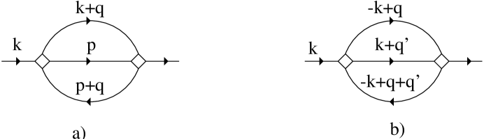
Figure 2: a) $q=0$ contribution to the self-energy; b) $q=2k_{F}$ contribution to the self-energy.

III.3 A non-analytic contribution to the self-energy from $q\approx 2k_{F}$

We next consider a singular contribution to $\Sigma_{R}^{\prime\prime}(\mathbf{k},\omega)$ from momentum transfers close to $2k_{F}$. To perform computations along the same lines as for Q near $0$, we would need to know the form of $\Pi(Q,\Omega)$ at finite $\Omega$ and $T$, which is rather involved. However, we actually would not need this form at all, as we demonstrate that the contribution to the self-energy from $Q\approx 2k_{F}$ is exactly the same as $\Sigma_{2}(\mathbf{k},\omega)$ defined in (31a). The most straightforward way to see this is to go back to a diagram representation of the self-energy in terms of three fermionic propagators (Fig.1c). In analytical form, the ${}^{\prime\prime}q=0^{\prime\prime}$ contribution to the self-energy is

$$\Sigma^{q=0}(k)=U^{2}\int\frac{d^{D+1}q}{\left(2\pi\right)^{D+1}}\int\frac{d^{D+1}p}{\left(2\pi\right)^{D+1}}G_{k+q}G_{p}G_{p+q}.$$ (45)

where $q$ is assumed to be small. We again use “relativistic” notation $k\equiv\left(\mathbf{k,}\omega\right)$ and $q\equiv\left(\mathbf{Q,}\Omega\right)$. Integrating over $p$ first, we obtain

$$\Sigma^{q=0}=-U^{2}\int\frac{d^{D+1}q}{\left(2\pi\right)^{D+1}}G_{k+q}\Pi(q),$$ (46)

where $\Pi(q)$ is a particle-hole bubble at small momentum and frequency. This expression we used in the previous subsection. We found that two singular contributions to $\Sigma^{q=0}$, $\Sigma_{1}(\mathbf{k},\omega)$ and $\Sigma_{2}(\mathbf{k},\omega)$, and that $\Sigma_{2}(\mathbf{k},\omega)$ comes from the momentum region where two of the internal momenta are close to $-\mathbf{k}$ and the third one is close to $\mathbf{k}$, i.e., from the range of $p$ which are nearly antiparallel to $k$. Since $p+k$ are small (of order of external momenta), we can relabel the momenta as shown in Fig. 2b and re-express $\Sigma_{2}(\mathbf{k},\omega)$ as

$$\Sigma_{2}(k)=U^{2}\int\frac{d^{D+1}q}{\left(2\pi\right)^{D+1}}\int\frac{d^{D+1}q^{\prime}}{\left(2\pi\right)^{D+1}}G_{k+q}G_{-k+q^{\prime}}G_{-k+q+q^{\prime}}.$$ (47)

where now both $q$ and $q^{\prime}$ are small. Integrating over $q^{\prime}$ first, we obtain a conventional expression for $\Sigma_{2}(k)$ in terms of the polarization operator with small momentum transfer. On the other hand, changing the order of integration and integrating over $q$ first, we obtain

$$\Sigma_{2}(k)=-U^{2}\int\frac{d^{D+1}q^{\prime}}{\left(2\pi\right)^{D+1}}~{}G_{-k+q^{\prime}}{\tilde{\Pi}}({2k-q^{\prime}})$$ (48)

where

$${\tilde{\Pi}}(2k-q^{\prime})=-\int\frac{d^{D+1}q}{\left(2\pi\right)^{D+1}}G_{k+q}G_{-k+q+q^{\prime}}.$$ (49)

In general, ${\tilde{\Pi}}(2k-q)$ is not equivalent to the polarization bubble $\Pi(q)$ with momentum near $2k_{F}$, as our re-writing is only valid if internal $q$ are small. However, the singular parts of the two bubbles coincide because the singular part in $\Pi(Q\approx 2k_{F},\Omega)$ (proportional to $\sqrt{|Q-2k_{F}|}\theta(|Q-2k_{F}|)$ in the static case) comes from the momentum range where the two internal momenta in the particle-hole bubble are close to $\pm\mathbf{k}$, i.e., from exactly the same range that is covered in ${\tilde{\Pi}}(2k-q^{\prime})$. We show this explicitly in the Appendix B. This equivalence implies that the r.h.s. of (48) is just the singular part of the “$2k_{F}$” contribution to the self-energy. We see therefore that $\Sigma^{q=2k_{F}}(k)=\Sigma_{2}^{q=0}(k)$. The total self-energy is then

$$\Sigma(k)=\Sigma^{q=0}(k)+\Sigma^{q=2k_{F}}=\Sigma_{1}(k)+2\Sigma_{2}(k).$$ (50)

For momentum-dependent interaction $U=U(q)$, the computation of the $2k_{F}-$contribution requires more care and we present it in Sec. VII.

That the $2k_{F}$-singularity comes from nearly antiparallel internal fermionic momenta has been implicitly used in the Kohn-Luttinger analysis of superconducting instability with large angular momenta of Cooper pairskl . In the context of corrections to the Fermi-liquid theory, Belitz et al. bkv argued that all singular contributions to the spin susceptibility can be described as small $q$ effects, although they did not emphasize that some of their small $q$ effects are in fact equivalent to $2k_{F}$ contributions in conventional notations.

That both $q=0$ and $q=2k_{F}$ singularities in the polarization bubble contribute to the self-energy was first emphasized by CM millis . However, the relative sign of the two terms is different in their and our calculations. We found that the singular terms add, while they argued that singular contributions from $q=0$ and $q=2k_{F}$ cancel each other. Since the interplay between $q=0$ and $q=2k_{F}$ contributions to the self-energy is crucial to the issue of whether or not there is a $T^{2}$-term in the specific heat and linear-in-$T$ term in the effective mass (CM argued that both are absent due to cancelation between $q=0$ and $q=2k_{F}$ terms), we present in Appendix B C an explicit computation of the $2k_{F}$ contribution to the second-order self-energy at $T=0$. This calculation confirms that $\Sigma^{q=2k_{F}}=\Sigma^{q=0}$.

III.4 An alternative analysis, in terms of $\Pi_{pp}(Q,\Omega)$

We next demonstrate that the backscattering non-analyticity in the fermionic self-energy can be viewed equivalently as coming from the non-analyticity in the particle-particle bubble at small total momentum and frequency. This readily follows from our consideration of the “$2k_{F}$” diagram. Indeed, since both $q$ and $q^{\prime}$ are small, the full self-energy can be re-expressed as

$$\Sigma(k)=-U^{2}\int\frac{d^{D+1}q}{\left(2\pi\right)^{D+1}}\int\frac{d^{D+1}q^{\prime}}{\left(2\pi\right)^{D+1}}G_{-k+q+q^{\prime}}\Pi_{pp}(q+q^{\prime}).$$ (51)

Performing the same analysis as in the previous section, we observe that the deviation from the Fermi-liquid form of $\Sigma$ is only possible if the expansion of $\Pi_{pp}^{\prime\prime}(Q,\Omega)$ in odd powers of $\Omega$ breaks down due to infrared divergences of momentum dependent prefactors. This is precisely what happens in $\Pi_{pp}(Q,\Omega)$ given by (19) as the frequency expansion holds in $\Omega/v_{F}Q$, i.e., the prefactors are non-analytic at vanishing $Q$. We emphasize that the logarithmic divergence of $\Pi_{pp}(\mathbf{Q},\Omega)$ at vanishing $Q$ and $\Omega$ is by itself not essential; what matters is a non-analytic dependence on the ratio $\Omega/v_{F}Q$.

We see, therefore, that the non-analytic piece in the self-energy can be viewed equivalently as coming from a non-analyticity in the particle-hole bubble, or from a non-analyticity in the particle-particle bubble. To further verify this, we explicitly compute in Appendix C the non-analytic part of $\Sigma(k)$ at $T=0$ using the “particle-particle formalism” and indeed find it to be equal to the non-analytic $2\Sigma_{2}(k,\omega)$ that we obtained in the “particle-hole formalism,” i.e.,

$$\Sigma_{pp}^{(Q=0)}(k)=2\Sigma_{2}(k).$$ (52)

The term $\Sigma_{1}(k,\omega)$ can be also reproduced in the particle-particle formalism, but this contribution comes from large $q+q^{\prime}\approx 2k$, and we refrain from re-deriving this piece.

Our results on this issue again disagree with those by CM  millis . They performed a complimentary analysis of the self-energy based on the evaluation of an effective vertex function to second order in $U$, and argued that there is a cancelation between non-analytic contributions coming from the $2k_{F}$ non-analyticity in the particle-hole channel and the non-analyticity in the particle-particle channel. We, on the contrary, find that the contribution from the particle-particle non-analyticity is twice the “$2k_{F}$” contribution from the particle hole channel.

Summarizing the results of the last two subsections, we see that the non-analytic part of the fermionic self-energy in 2D consists of two parts. The first part, $\Sigma_{1}^{\prime\prime}(k)$, comes from forward scattering. It has the same functional form, $\omega^{2}+(\pi T)^{2}$, as in a Fermi liquid, but the prefactor logarithmically depends on $\omega-\epsilon_{k}$. The second part, $\Sigma_{2}^{\prime\prime}(k)$, comes from the processes which involve the scattering amplitude with near-zero total and transferred momentum. This $\Sigma_{2}^{\prime\prime}(k)$ has a non-Fermi-liquid form, and can be equally attributed to the $Q=0$ non-analyticity in the particle-hole polarization bubble, or to the $2k_{F}$ non-analyticity in the same bubble, or to the $Q=0$ singularity in the particle-particle bubble. In the next section we show that only $\Sigma_{2}(k)$ actually contributes to the thermodynamics.

III.5 Effective Mass and Specific Heat

We first use the result for $\Sigma^{\prime\prime}$ obtained in Sec.III.2 and compute the real part of the self-energy on the mass shell. We then use $\Sigma^{\prime}(\omega=\epsilon_{k})$ to find the effective mass and specific heat.

The Kramers-Kronig relation on the mass shell is

$$\Sigma_{R}^{\prime}(\omega)=\frac{1}{\pi}\mathcal{P}\int dE\frac{\Sigma^{\prime\prime}(E,\epsilon_{k}=\omega)}{E-\omega}.$$ (53)

We begin with $\Sigma_{1}(k)$. Substituting $\Sigma_{1}^{\prime\prime}(\mathbf{k},\omega)$ from (31b)into (53), we find that on the mass shell

$$\Sigma_{1}^{\prime}(k,\omega)|_{\omega=\epsilon_{k}}=\frac{mU^{2}}{16\pi^{4}v_{F}^{2}}\mathcal{P}\int_{-\infty}^{\infty}dz\frac{z^{2}+(\pi T)^{2}}{z-\omega}~{}\ln\frac{W}{|z-\omega|}.$$ (54)

By dimensional analysis, the integral in (54) is of order $\omega^{2}$. However, the prefactor in front of $\omega^{2}$ turns out to be zero. The easiest way to see this is to evaluate the integral in finite limits $-W<z<W$ and to search for the universal term that would be independent of $W$. Performing elementary manipulations, we find that $\Sigma_{1}^{\prime}(\omega)$ does not contain such a term. Foreshadowing, we note that the same result holds for the static spin susceptibility which we discuss in detail in Sections IV.1 and IV.2. We will see there that the inclusion of the $\Sigma_{2}(k,\omega)$ into a particle-hole bubble with external momentum $Q$ yields a non-analytic $|Q|$ term in $\chi_{s}(Q)$. On the contrary, the susceptibility diagram with an extra $\Sigma_{1}(\mathbf{k},\omega)$ scales, in Matsubara frequencies, as

$$\delta\chi\propto\int d\omega_{n}\omega_{n}\int d\epsilon_{k}\frac{\ln\left[W/\left(\epsilon{{}_{k}-}i\omega_{n}\right)\right]}{(\epsilon_{k}-i\omega_{n})^{2}\left[(\epsilon_{k}-i\omega_{n})^{2}-(v_{F}Q)^{2}\right]}.$$ (55)

By power counting, the leading $Q$ dependence of the integral should be $|Q|$. However, a straightforward computation shows that the prefactor again vanishes. The outcome of this analysis is that the divergence of $\Sigma_{1}^{\prime\prime}(\mathbf{k},\omega)$ on the mass shell does not give rise to non-analytic corrections to Fermi-liquid form of the thermodynamic observables.

We next consider $\Sigma_{2}^{\prime}(\mathbf{k},\omega)$. Substituting $\Sigma_{2}^{\prime\prime}(\mathbf{k},\omega)$ from Eq.(40) into Eq.(53), we obtain after simple manipulations

$$\Sigma_{2}^{\prime}(\omega) = -\frac{mU^{2}}{16\pi^{4}v_{F}^{2}}~{}\omega~{}\int_{-\infty}^{\infty}d\Omega\Omega\text{ }\mathcal{P}\int_{0}^{\infty}\frac{dE}{E^{2}-\omega^{2}}~{}\left(\coth\frac{\Omega}{2T}-\tanh\frac{\Omega+E}{2T}\right)$$ (56)

$$~{}\left(\frac{E}{\omega}\ln\left|\frac{2\Omega+E-\omega}{2\Omega+E+\omega}\right|+\ln\frac{|(2\Omega+E)^{2}-\omega^{2}|}{W^{2}}\right).$$

Integrations over $\Omega$ and $E$ can be performed exactly. We give the details of this calculation in Appendix D and present just the results here. At $T=0$, we obtain

$$\Sigma_{2}^{\prime}(\omega)=-\frac{mU^{2}}{32\pi^{2}v_{F}^{2}}\omega|\omega|.$$ (57)

This coincides with Eq.(39) obtained via analytic continuation of the Matsubara self-energy.

In the opposite limit of small $\omega/T$, we have

$$\Sigma_{2}^{\prime}(\omega)=~{}-~{}\frac{mU^{2}\ln 2}{8\pi^{2}v_{F}^{2}}~{}~{}\omega T.$$ (58)

As the self-energy in this region is linear in $\omega,$ Eq. (58) implies that the effective mass of subthermal quasiparticles, i.e., with $\omega\ll T,$ scales linearly with $T$. Using the fact that the full $\Sigma(k,\omega)=\Sigma_{1}(k,\omega)+2\Sigma_{2}(k,\omega)$ and that $\Sigma_{1}(k,\omega)$ does not contribute to thermodynamics, we obtain

$$m^{\ast}(T)=m^{\ast}(T=0)\left(1-2\ln 2\left(\frac{mU}{4\pi}\right)^{2}\frac{T}{E_{F}}\right).$$ (59)

This result disagrees with CM–they argued that the linear-in-$T$ term in the mass renormalization is absent.

In a very recent study Das Sarma, Galitski, and Zhang dassarma_mass did find a linear-in-T correction to the effective mass for the Coulomb interaction in $D=2$. Although the sign of their linear-in-$T$ term is opposite to that in Eq.(59), we believe that there is no contradiction here as there are no general restrictions on the sign of the prefactor. It is therefore quite possible that the sign of the $O(T)$ term is different for short- and long-range interactions. Note in this regard that the effect of the interaction on the effective mass is different for these two cases even at $T=0$ : a short-range interaction increases $m^{*}$, while the Coulomb interaction decreases $m^{*}$ in the limit $r_{s}\ll 1$ agd .

For generic $\omega/T$, the non-analytic part of the full $\Sigma^{\prime}(\omega)$ can be cast into the following scaling form

$$\Sigma^{\prime}(\omega)=-\frac{mU^{2}}{16\pi^{2}v_{F}^{2}}\omega|\omega|g\left(\frac{|\omega|}{T}\right),$$ (60)

where

$$g(x)=1+\frac{4}{x^{2}}\left[\frac{\pi^{2}}{12}+\text{Li}_{2}\left(-e^{-x}\right)\right],$$ (61)

and Li${}_{2}(x)$ is a polylogarithmic function.

Note that $g(\infty)=1$ and $g(x\ll 1)\approx 4\ln 2/x$. Substituting these limiting expressions into Eq.(60) we indeed reproduce Eq.(57) and Eq.(58).

The full functional form of $g(x)$ is required for the computation of the specific heat, as the frequency integral for $C(T)$ given by Eq.(4) is confined to $\omega\sim T$. Previous work  previous_C(T) on $C(T)$ used only the $T=0$ form of the self-energy and hence yielded incorrect prefactors. Substituting our result for $\Sigma^{\prime}$ into (4) we obtain in 2D

$$\delta C(T)=C_{FL}\frac{48K}{\pi}~{}\left(\frac{mU}{4\pi}\right)^{2}\frac{T}{E_{F}},$$ (62)

where $C_{FL}(T)=m\pi T/3$ is the Fermi gas result for the specific heat and

$$K=\int_{0}^{\infty}\frac{dxx}{\cosh^{2}x}~{}\left[x^{2}+\frac{\pi^{2}}{12}+\text{Li}_{2}\left(-e^{-2x}\right)\right]=1.803.$$ (63)

As it was to be anticipated, the non-analytic correction to the fermionic self-energy gives rise to the $T^{2}$-term in the specific heat. It is essential that this non-analytic term comes only from fermions in a near vicinity of the Fermi surface and is thus model-independent. The same is true for the linear-in-$T$ correction to the effective mass. In other words, the leading corrections to the Fermi-liquid forms of $m$ and $C(T)$ are fully universal.

The $T^{2}$-dependence of the correction to the specific heat agrees with the results by Coffey and Bedell bedell and Misawa misawa . However, Coffey and Bedell did not explicitly compute the prefactor and apparently only included small momentum transfers (i.e., no $2k_{F}$ effects). Misawa did compute the prefactor, but he neglected the temperature dependence of the fermionic self-energy. We found above that this $T$ dependence cannot be neglected, and our prefactor disagrees with that by Misawa.

III.6 Amplitude of quantum magneto-oscillations

In previous sections, we found the general form of non-analytic corrections to the real and imaginary parts of the self-energy. We now discuss whether these corrections can be observed experimentally via magneto-oscillations. Naively speaking, one might have expected the finite quasiparticle relaxation rate, $T^{2}\ln T,$ to damp the amplitude of the oscillations as a contribution to the “Dingle temperature”, whereas the $T-$ dependent effective mass might affect the thermal smearing factor. However, we argue below that quadratic and quadratic-times-log terms in the self-energy are not detectable by measuring the amplitude of magneto-oscillations in $D=2$.

In the Luttinger formalism luttinger , the amplitude of the $k^{th}-$ harmonic of magneto-oscillations is given by

$$A_{k}=\frac{4\pi^{2}kT}{\Omega_{c}}\sum_{\omega_{n}>0}\exp\left(-\frac{2\pi k\left[\omega_{n}-i\Sigma\left(\omega_{n},T\right)\right]}{\Omega_{c}}\right),$$ (64)

where $\Omega_{c}$ is the cyclotron frequency. It is essential for our consideration that the amplitude is determined by the self-energy in the Matsubara representation rather than by the real and imaginary parts of the retarded self-energy engelsberg . By itself, $\Sigma_{R}^{\prime}$ and $\Sigma_{R}^{\prime\prime}$ determine the fermion dispersion and lifetime, respectively; however in (64) this distinction is lost.

The assumption made in deriving (64) is that the dependence of the self-energy on the magnetic field can be neglected. In 3D, this assumption is well justified as the effect of the magnetic field on the self-energy yields corrections to $A_{k}$ which are small in $1/\sqrt{N},$ where $N=\epsilon_{F}/\Omega_{c}\gg 1$ is the total number of Landau levels. In 2D, however, the effect of the magnetic field is non-perturbative, and at $T=0$ and in the absence of disorder, the field-induced oscillations of the self-energy are as important as the oscillations of the thermodynamic potential itself curnoe . Eq.(64) is then only applicable as long as oscillations of the thermodynamic potential are exponentially small due to either finite temperature and/or disorder. In this paper we disregard effects of disorder (considered recently in maslov ), thus the amplitude is only controlled by the finite temperature. In this case, the restriction of the small amplitude in its turn implies that the sum over Matsubara frequencies in (64) can be truncated to only the $n=0$ term. Notice that this restriction is mandatory in $D=2$ within the Luttinger formalism but depends on the choice of experimental conditions in $D=3.$ The amplitude of the first (largest) harmonic then simplifies to

$$A_{1}=\frac{4\pi^{2}T}{\Omega_{c}}\exp\left(-\frac{2\pi\left[\pi T-i\Sigma\left(\pi T,T\right)\right]}{\Omega_{c}}\right).$$ (65)

The temperature enters the Matsubara self-energy $\Sigma\left(\omega_{n},T\right)$ in two ways: first, as the Matsubara frequency, and second, as the physical temperature determining the thermal distribution of the degrees of freedom. For the lowest frequency, $\omega_{0}=\pi T$, the interplay between the two effects leads to a peculiar cancelation.

Indeed, consider for a moment a generic Fermi liquid, for which

$$\Sigma\left(\omega_{n},T\right)=\left(\frac{m^{\ast}}{m}-1\right)i\omega_{n}+iC\left[\left(\pi T\right)^{2}-\omega_{n}^{2}\right]+\dots,$$ (66)

where $C$ is a constant, $\dots$ stand for the higher order terms $\left[\mathcal{O}\left(\epsilon_{n}^{3},T^{3}\right)\right]$, and $m^{\ast}/m$ has a regular expansion in powers of $T^{2}$. The analytic continuation of (66) to real frequencies yields the correct retarded self-energy (1). We see that the second term $\Sigma\left(\omega_{n},T\right)$ vanishes for $\omega_{n}=\pm\pi T$, i.e., the self-energy that enters into the formula for $A_{k}$ contains terms only of order $T^{3}$ and higher. In other words, the quadratic in $T$ piece present in the imaginary part of the retarded self-energy and associated observables, does not affect the amplitude of magneto-oscillations, which to order $T^{3}$ is given by

$$A_{1}=\frac{4\pi^{2}T}{\Omega_{c}}\exp\left(-\frac{2\pi^{2}T}{\Omega_{c}^{\ast}}\right),\text{ }\Omega_{c}^{\ast}\equiv\frac{m}{m^{\ast}}\Omega_{c},$$ (67)

where $m^{\ast}/m$ is a regular mass renormalization which comes from fermions far away from the Fermi surface. This rather remarkable result was previously obtained specifically for electron-phonon interaction and is known as a “Fowler-Prange theorem” prange .

We found that a similar cancelation occurs also for our self-energy in $D=2$. To logarithmic accuracy, the second term in Eq.(66) is replaced by

$$\tilde{\Sigma}\left(\omega_{n},T\right)=-i{\tilde{C}}~{}T\sum_{\Omega_{m}}\text{sgn}\left(\omega_{n}-\Omega_{m}\right)\left|\Omega_{m}\right|\ln\frac{\left|\Omega_{m}\right|}{W},$$ (68)

where ${\tilde{C}}$ is a real constant, and the factor of sgn$\left(\omega_{n}-\Omega_{m}\right)$ resulted from the angular integration of the Green’s function. A simple transformation of the Matsubara sum reduces $\tilde{\Sigma}\left(\omega_{n},T\right)$ to

$$\tilde{\Sigma}\left(\omega_{n},T\right)=-2iT{\tilde{C}}~{}\sum_{\Omega_{m}=0}^{\omega_{n}-\pi T}\Omega_{m}\ln\frac{\Omega_{m}}{W}.$$ (69)

Expression (69) obviously vanishes for $\omega_{n}=\pi T$, i.e., therefore $\Sigma\left(\pi T,T\right)$ in (65) does not contain a contribution from $\tilde{\Sigma}.$ Due to this cancelation, the exponential factor in $A_{1}$ does not contain terms of order $T^{2}\ln T$. A more detailed analysis maslov , shows that $T^{2}$ terms are also absent, i.e., both quadratic terms and quadratic-times-log terms in the self-energy (and thus the linear-in-$T$ effective mass [Eq.(59) ]) are not observable in a magneto-oscillation experiments.

IV spin and charge susceptibilities

We next proceed to the analysis of the corrections to the Fermi-liquid forms of spin and charge susceptibilities.

The charge and spin operators are bilinear combinations of fermions:

$$C(q)=\sum_{\mathbf{k},\alpha}c_{\mathbf{k}+\mathbf{q},\alpha}^{\dagger}c_{\mathbf{k},\alpha}$$ (70)

for charge, and

$${\vec{S}}(q)=\sum_{\mathbf{k},\alpha,\beta}{\vec{\sigma}}_{\alpha\beta}c_{\mathbf{k}+\mathbf{q},\alpha}^{\dagger}c_{\mathbf{k},\beta}$$ (71)

for spin. The corresponding susceptibilities for a system of interacting fermions are given by fully renormalized particle-hole bubbles with side vertices

$$\Gamma_{c}=\delta_{\alpha,\beta};~{}~{}\Gamma_{s}^{i}=\sigma_{\alpha,\beta}^{i},$$ (72)

where $c$ and $s$ refer to charge and spin, respectively.

For non-interacting fermions, the spin and charge susceptibilities are equal and given by the Lindhard function that coincides, up to an overall factor, with the polarization operator $\Pi(Q,\Omega_{m})$:

$$\chi_{0}^{c}(Q,\Omega_{m})=\chi_{0}^{s}(Q,\Omega_{m})=2\Pi(Q,\Omega_{m}),$$ (73)

where $\chi_{0}^{s}(Q,\Omega_{m})\equiv\left[\chi_{0}^{s}(Q,\Omega_{m})\right]_{ii}$ and $i=1,2,3,$ and

$$\Pi(Q,\Omega_{m}) = -T\sum_{m}\int\frac{d^{D}k}{(2\pi)^{d}}~{}$$ (74)

$$G_{0}(\mathbf{k},\omega_{n})~{}G_{0}(\mathbf{k}+\mathbf{Q},\omega_{n}+\Omega_{m}).$$

At $T=0,$the charge and spin susceptibilities can be evaluated exactly for any $Q$ and $\Omega_{m}.$ In the static limit, $\Omega_{m}=0,$ they acquire particularly simple forms. For $D=3$, we have ashcroft_mermin

$$\chi_{0}^{c}(Q,0)=\chi_{0}^{s}(Q,0)=\chi_{0}^{3D}\left[\frac{1}{2}+\frac{4k_{F}-Q^{2}}{8Qk_{F}}\ln{\frac{Q+2k_{F}}{|Q-2k_{F}|}}\right],$$ (75)

where $\chi_{0}^{3D}=mk_{F}/\pi^{2}$. In $D=2$, the corresponding expression is kagan ; stern_1

$$\chi_{0}^{c}(Q,0) = \chi_{0}^{s}(Q,0)=\chi_{0}^{2D},~{}~{}Q<2k_{F};$$

$$\chi_{0}^{c}(Q,0) = \chi_{0}^{s}(Q,0)=\chi_{0}^{2D}\left[1-\left(1-\frac{4k_{F}^{2}}{Q^{2}}\right)^{1/2}\right],~{}~{}Q>2k_{F},$$ (76)

where $\chi_{0}^{2D}=m/\pi$. In 1D, we have DL_1

$$\chi_{0}^{c}(Q,0)=\chi_{0}^{s}(Q,0)=\chi_{0}^{1D}\frac{k_{F}}{Q}~{}\ln\left|\frac{k_{F}+\frac{Q}{2}}{k_{F}-\frac{Q}{2}}\right|,$$ (77)

where $\chi_{0}^{1D}=2/(\pi v_{F}).$ As it was mentioned in the Introduction, $\chi_{0}^{c,s}(Q,0)$ is analytic in $Q$ for small $Q$ in all dimensions.

The first nontrivial corrections to $\chi_{0}^{c,s}(Q,0)$ come from the diagrams presented in Fig.3. These diagrams represent self-energy and vertex-correction insertions into the bare particle- hole bubble bkv . Diagrams $1-5$ are nonzero for both $\chi_{s}$ and $\chi_{c}$. Diagrams $6$ and $7$ are finite for $\chi_{c}$, but vanish for $\chi_{s}$ upon the spin summation ($\sum_{\alpha}\sigma_{\alpha\alpha}^{i}=0$). The internal parts of all diagrams contain fermionic bubbles: particle-hole bubbles for diagrams $1,2,3,5$ and particle-particle bubble for the diagram $4$.

In the next two sections we analyze the form of the static susceptibility first at a finite $Q$ and zero temperature, and then at finite $T$ and $Q=0$.

IV.1 Spin and charge susceptibilities at finite $Q$ and $T=0$

As in Sec. III, we assume that the interaction is independent of momentum. We explicitly computed all $7$ diagrams Fig. 3 and found that each of the diagrams (except for diagrams 6 and 7 which vanish identically for the spin channel) contributes a correction $\delta\chi(Q,0)\propto|Q|$, and that this non-analyticity is a direct consequence of the dynamical singularities in the particle-hole and particle-particle bubbles.

IV.1.1 $D=2$

As we mentioned in the Introduction, the calculation in $D=2$ is more difficult to perform than in $D=3$ because all typical internal momenta and energies are of the same order as the external ones ($Q$ and $v_{F}Q$, respectively); thus no expansion is possible. In 3D, where $\delta\chi(Q,0)\propto Q^{2}\ln Q$, typical internal momenta are larger than external $Q$, and one could expand the integrand in $Q^{2}$ and evaluate the prefactor to logarithmic accuracy.

We begin with diagram 1 which represents the self-energy insertion into the particle-hole bubble. This diagram yields the same contribution for spin and charge channels, so we will drop the subscript and denote $\chi_{1}\equiv\chi_{1s}=\chi_{1c}$.

Figure 3: Each of  the seven diagrams in this figure give singular corrections to spin and charge susceptibilities.

An analytic form of diagram 1 in the Matsubara representation is given by

$$\delta\chi_{1}(Q,0)=-8U^{2}\int\frac{d^{2}k~{}d^{2}q~{}d\omega d\Omega}{(2\pi)^{6}}G_{0}^{2}(\mathbf{k},\omega)G_{0}(\mathbf{k}+\mathbf{Q},\omega)G_{0}(\mathbf{k}+\mathbf{q},\omega+\Omega)\Pi(q,\Omega).$$ (78)

The combinatorial factor of $8$ includes two factors of $2$ due to spin summation and an extra factor of $2$ associated with the fact that the self-energy can be added to any of the two fermionic lines in the bubble. Non-analytic contributions to $\delta\chi_{1}(Q,0)$ come from two regions of momentum transfers: $q$ near zero and $q$ near $2k_{F}$. Since we have already shown in Sec. III that the contributions to the self-energy from these two regions are equal for a contact interaction (up to a forward scattering piece in $\Sigma^{q=0}$ that, as we demonstrated, does not contribute to $|Q|$ term in the susceptibility), we do not have to calculate the $q=0$ and $q=2k_{F}$ contributions to $\chi_{1}(Q,0)$ separately–the two are just equal:

$$\delta\chi_{1}^{q=0}(Q,0)=\delta\chi_{1}^{q=2k_{F}}(Q,0).$$ (79)

This implies that we only have to compute $\delta\chi_{1}^{q=0}(Q,0)$, the full $\delta\chi_{1}(Q,0)$ will be twice that value. To be on a safe side, we verified this reasoning by explicitly computing $\delta\chi_{1}^{q=2k_{F}}(Q,0)$. We present the calculations in Appendix E. We indeed found it to be equal to $\delta\chi_{1}^{q=0}(Q,0)$.

We now compute $\delta\chi_{1}^{0}(Q,0)$ Since the non-analyticity in $\chi_{1}(Q,0)$ is expected to come from the vicinity of the Fermi surface, the fermionic spectra $\epsilon_{k}$, $\epsilon_{k+q}$ and $\epsilon_{k+Q}$ can be expanded to first order in $k-k_{F}$:

$$\epsilon_{\mathbf{k}}=v_{F}(k-k_{F}),~{}~{}\epsilon_{\mathbf{k}+\mathbf{Q}}=\epsilon_{k}+v_{F}Q\cos{\theta_{1}},~{}~{}\epsilon_{\mathbf{k}+\mathbf{q}}=\epsilon_{k}+v_{F}q\cos{\theta_{2}}.$$ (80)

Substituting this expansion into Eq.(78) and performing elementary integrations over $k$, $\omega$, and $\theta_{1}$, we obtain

$$\delta\chi_{1}^{q=0}(Q,0) = -\frac{2mU^{2}}{\pi^{4}}~{}\int_{0}^{\infty}qdq\int_{0}^{\infty}{\Omega}d{\Omega}\Pi(q,\Omega)$$ (82)

$$\times\int_{0}^{\pi}d\theta_{2}~{}\frac{1}{(i{\Omega}-v_{F}q\cos\theta_{2})^{2}}~{}\frac{1}{\sqrt{(v_{F}Q)^{2}+({\Omega}+iv_{F}q\cos\theta{{}_{2}})^{2}}},$$

where $\Pi(q,\omega)$ at small $q$ and $\omega$ is given by Eq.(13). Rescaling the remaining variables as ${\tilde{q}}=q/Q,~{}{\tilde{\omega}}=\Omega/(v_{F}Q)$ and introducing polar coordinates as ${\tilde{q}}=r\cos\phi,{\tilde{\Omega}}=r\sin\phi$, we obtain from (82)

$$\delta\chi_{1}^{q=0}(Q,0) = -\frac{2mU^{2}|Q|}{\pi^{4}v_{F}}~{}\int_{0}^{\pi/2}d\phi\sin\phi\cos\phi\Pi(\phi)$$

$$\int_{0}^{\pi}d\theta_{2}~{}\int rdr~{}\frac{1}{(\cos\phi~{}\cos\theta_{2}-i\sin\phi)^{2}}~{}\frac{1}{\sqrt{1+r^{2}(\sin\phi+i\cos\phi~{}\cos{\theta_{2}})^{2}}},$$

where $\Pi(\phi)=(m/2\pi)(1-\sin\phi)$. The upper limit of the integral over $r$ is $r_{max}=\mathcal{O}(k_{F}/Q)\gg 1$. The integration over $r$ is straightforward and yields

$$\delta\chi_{1}^{q=0}(Q,0) = \frac{2mU^{2}}{\pi^{4}v_{F}}~{}\int_{0}^{\pi/2}d\phi\sin\phi\cos\phi\Pi(\phi)\int_{0}^{\pi}d\theta_{2}~{}\frac{1}{(\cos\phi~{}\cos\theta_{2}-i\sin\phi)^{4}}$$

$$\times\left[\sqrt{Q^{2}+(Q~{}r_{max})^{2}(\sin\phi+i\cos\phi~{}\cos{\theta_{2}})^{2}}-|Q|\right].$$

As $Q~{}r_{max}\sim k_{F}$, the dominant piece in $\delta\chi_{1}^{q=0}(Q,0)$ comes from high energies and accounts for the non-universal correction to the uniform susceptibility $\chi(0,0)$. We, however, are interested in the first subleading term which scales as $|Q|$ and does not depend on $r_{max}$. Performing the integration over $\theta_{2}$, we obtain for this universal contribution

$$\delta\chi_{1}^{q=0}(Q,0)=-\frac{mU^{2}|Q|}{\pi^{3}v_{F}}~{}\int_{0}^{\pi/2}d\phi\sin^{2}{\phi}\cos{\phi}~{}(5\sin^{2}\phi-3)~{}\Pi(\phi).$$ (85)

Finally, introducing $z=\cos\phi$ [so that $\Pi(z)=(m/2\pi)(1-z)]$, we obtain

$$\delta\chi_{1}^{q=0}(Q,0)=-\frac{m^{2}U^{2}|Q|}{2\pi^{4}v_{F}}~{}\int_{0}^{1}dz~{}(5z^{4}-3z^{2})~{}(1-z).$$ (86)

The relevance of the non-analyticity in the polarization bubble is now transparent: if $\Pi(z)$ was $z$-independent, the integral over $z$ would vanish. However, because of the non-analyticity, $\Pi(z)$ varies linearly with $z$. The integral over $z$ then does not vanish, and performing the integration we obtain

$$\delta\chi_{1}^{q=0}(Q,0)=\chi_{0}~{}\frac{2}{3\pi}~{}\left(\frac{mU}{4\pi}\right)^{2}~{}\frac{|Q|}{k_{F}},$$ (87)

where $\chi_{0}=2\Pi(0,0)=m/\pi$ is the static susceptibility of noninteracting fermions.

Using (79), we then obtain the total contribution of diagram 1:

$$\delta\chi_{1}(Q,0)=2\delta\chi_{1}^{q=0}(Q,0)=\chi_{0}~{}\frac{4}{3\pi}~{}\left(\frac{mU}{4\pi}\right)^{2}~{}\frac{|Q|}{k_{F}}.$$ (88)

Diagram 2 is another self-energy insertion into the particle-hole bubble. For a contact interaction, $\delta\chi_{2}$ is exactly $(-1/2)$ of $\delta\chi_{1}$, the rescaling factor $-1/2$ comes from the fact that compared to diagram 1, diagram 2, has one lass fermionic loop with more than one vertex, and lacks the factor of two due to spin summation. Therefore

$$\delta\chi_{2}(Q,0)=-\chi_{0}~{}\frac{2}{3\pi}~{}\left(\frac{mU}{4\pi}\right)^{2}~{}\frac{|Q|}{k_{F}}.$$ (89)

The next diagram, diagram 3, represents a vertex correction to the particle-hole bubble. The $q=0$ contribution to this diagram can be shown to be of the same magnitude but opposite sign as the $q=0$ part of diagram 1. To see this, we write the $q=0$ contribution to diagram 3 as

$$\delta\chi_{3}^{q=0}(Q,0) = -4U^{2}\int\int\int\int\frac{d^{2}k~{}d^{2}q~{}d\omega d\Omega}{(2\pi)^{6}}G_{0}(\mathbf{k},\omega)G_{0}(\mathbf{k}+\mathbf{q},\omega+\Omega)$$ (91)

$$\times G_{0}(\mathbf{k}+\mathbf{Q}+\mathbf{q},\omega+\Omega)G_{0}(\mathbf{k}+\mathbf{Q},\omega)\Pi(q,\Omega)$$

and consider a combination

$$C=\frac{1}{2}\delta\chi_{1}^{q=0}+\delta\chi_{3}^{q=0}.$$ (92)

Linearizing the fermionic spectra according to Eq.(80), we re-write $C$ as

$$C=-4U^{2}\nu_{1}\int\int\int\frac{d^{2}qd\omega d\Omega}{\left(2\pi\right)^{4}}\int d\theta_{1}\Pi\left(q,\Omega\right)\left[S_{1}+S_{3}\right],$$ (93)

where

$$S_{1}=\int d\epsilon_{k}G_{0}^{2}(\mathbf{k},\omega)G_{0}(\mathbf{k}+\mathbf{Q},\omega)G_{0}(\mathbf{k}+\mathbf{q},\omega+\Omega)$$ (94)

and

$$S_{3}=\int d\epsilon_{k}G_{0}(\mathbf{k},\omega)G_{0}(\mathbf{k}+\mathbf{q},\omega+\Omega)G_{0}(\mathbf{k}+\mathbf{Q}+\mathbf{q},\omega+\Omega)G_{0}(\mathbf{k}+Q,\omega).$$ (95)

Integrating over $\epsilon_{k}$ in Eqs.(94,95) yields

$$S_{1} = -2\pi i\text{sgn}\left(\Omega\right)\theta\left(\omega\left(\Omega-\omega\right)\right)\frac{1}{\left(i\Omega+v_{F}\mathbf{\hat{k}}\cdot\mathbf{q}\right)^{2}}\frac{1}{i\Omega+v_{F}\mathbf{\hat{k}}\cdot\mathbf{q-}v_{F}\mathbf{\hat{k}}\cdot\mathbf{Q}},$$

$$S_{3} = 2\pi i\text{sgn}\left(\Omega\right)\theta\left(\omega\left(\Omega-\omega\right)\right)\frac{1}{v_{F}\mathbf{\hat{k}}\cdot\mathbf{Q}}\frac{1}{i\Omega+v_{F}\mathbf{\hat{k}}\cdot\mathbf{q}}$$

$$\times\left(\frac{1}{i\Omega+v_{F}\mathbf{\hat{k}}\cdot\mathbf{q-}v_{F}\mathbf{\hat{k}}\cdot\mathbf{Q}}-\frac{1}{i\Omega+v_{F}\mathbf{\hat{k}}\cdot\mathbf{Q}}\right).$$

Adding $S_{1}$ and $S_{3}$ and performing some elementary transformations, we obtain

$$S_{1}+S_{3}=2\pi i\text{sgn}\left(\Omega\right)\theta\left(\omega\left(\Omega-\omega\right)\right)\frac{1}{\left(i\Omega+v_{F}\mathbf{\hat{k}}\cdot\mathbf{q}\right)^{2}}\frac{1}{i\Omega+v_{F}\mathbf{\hat{k}}\cdot\mathbf{q+}v_{F}\mathbf{\hat{k}}\cdot\mathbf{Q}}.$$

Substituting the last expression back into Eq.(93) and making the change of variables $\mathbf{k\rightarrow-k,}$ $\mathbf{q\rightarrow-q}$ results in

$$C=-\frac{1}{2}\delta\chi_{1}^{q=0},$$ (96)

Together with (92), this proves that

$$\delta\chi_{3}^{q=0}(Q,0)=-\delta\chi_{1}^{q=0}(Q,0)=-\chi_{0}~{}\frac{2}{3\pi}~{}\left(\frac{mU}{4\pi}\right)^{2}~{}\frac{|Q|}{k_{F}}.$$ (97)

The $2k_{F}$-contribution from diagram 3 must be computed independently. The computations are performed along the same lines as for diagram 1. We present them in the Appendix E. We obtain

$$\delta\chi_{3}^{2k_{F}}(Q,0)=\chi_{0}~{}\frac{2}{3\pi}~{}\left(\frac{mU}{4\pi}\right)^{2}~{}\frac{|Q|}{k_{F}}.$$ (98)

Comparing this with Eq.(89), we see that, for a constant interaction, the $\mathcal{O}(|Q|)$ contributions to diagram 3 from the singularities at $q=0$ and $q=2k_{F}$ cancel each other. This result appears to be quite general (the same is true for $D=3$ and $D=1$ also (see below), but we do not know how to prove it other than to explicitly compute the diagrams.

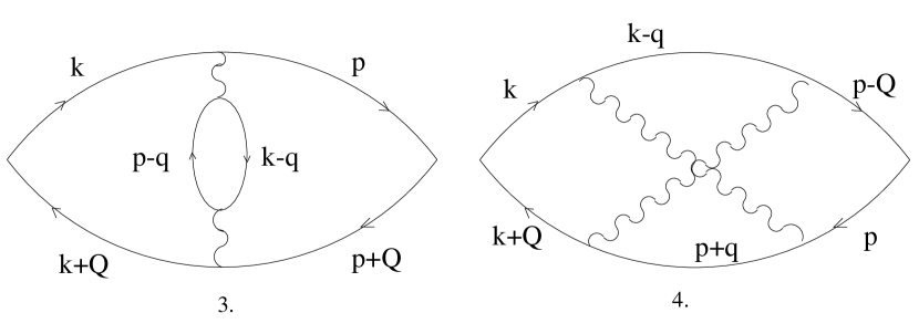
Figure 4: A reduction of $\delta\chi_{4}$ to the $2k_{F}$ part of $\delta\chi_{3}.$

Next we consider diagram 4, which is obtained by inserting the particle-particle bubble into the original particle-hole bubble. Expressing $\delta\chi_{4}$ via the product of four Greens’s functions and the particle-particle bubble, we obtain

$$\delta\chi_{4}(Q,0) = -2U^{2}\int\int\int\int\frac{d^{2}k~{}d^{2}q~{}d\omega d\Omega}{(2\pi)^{6}}G_{0}(\mathbf{k},\omega)G_{0}(\mathbf{k}+\mathbf{Q},\omega)$$ (99)

$$\times G_{0}(\mathbf{q}-\mathbf{k},\Omega-\omega)G_{0}(\mathbf{q}-\mathbf{k}-\mathbf{Q},\Omega-\omega)\Pi_{pp}(q,\Omega),$$

where $\Pi_{pp}(q,\Omega)$ is given by (19).

In principle the result for $\delta\chi_{4}$ can be found by substituting the particle-particle propagator into (99). However, a straightforward approach is very cumbersome in this case. There is a more elegant way to compute $\delta\chi_{4}$ as the non-analytic part of this diagram is related to the non-analytic $2k_{F}$ contribution from diagram 3, which we have already found. Indeed, it is easy to make sure that a non-analytic $(\propto|Q|)$ contribution from diagram 4 comes from internal momenta for which one of the internal 3-momentum transfers is small. We can then label the internal momenta in diagram 4 as shown in Fig. 4 and set 3-momentum $q$ to be small (there is a combinatorial factor of $2$ associated with this choice). We can then represent diagram 3 as an integral-over-$q$ of a product of two terms (“triads”) each containing a product of three Green’s functions:

$$\delta\chi_{4}=-2\times 2U^{2}\int\int\frac{d^{2}qd\Omega}{\left(2\pi\right)^{3}}I\left(\mathbf{q},\Omega;\mathbf{Q}\right)I\left(-\mathbf{q},-\Omega;-\mathbf{Q}\right),$$ (100)

where a “triad” is defined as

$$I\left(q,\Omega;Q\right)=\int\int\frac{d^{2}kd\omega}{\left(2\pi\right)^{3}}G\left(\mathbf{k},\omega\right)G\left(\mathbf{k-q,}\omega-\Omega\right)G\left(\mathbf{k+Q,}\omega\right).$$ (101)

An extra overall factor of $-2$ in (102) is due to spin summation and the presence of one closed fermionic loop. At the same time, we can use the fact that in the $2k_{F}$ part of diagram 3, one of the two momenta in the internal particle-hole bubble is close to incoming ones. Using the labeling as in Fig. 4, we can express the $2k_{F}$ part of diagram 3 as

$$\delta\chi_{3}^{2k_{F}}=4U^{2}\int\int\frac{d^{2}qd\Omega}{\left(2\pi\right)^{3}}\left[I\left(\mathbf{q},\Omega;\mathbf{Q}\right)\right]^{2},$$ (102)

Carrying out integrations over $\epsilon_{k}$ and $\omega$ in Eq.(101), we find that

$$I\left(-\mathbf{q},-\Omega;\mathbf{Q}\right)=-I\left(\mathbf{q},\Omega;\mathbf{Q}\right),$$ (103)

and hence

$$\delta\chi_{4}(Q,0)=\delta\chi_{3}^{2k_{F}}(Q,0)=\chi_{0}~{}\frac{2}{3\pi}~{}\left(\frac{mU}{4\pi}\right)^{2}~{}\frac{|Q|}{k_{F}}.$$ (104)

Similarly, diagram 5 differs by a factor of $-1$ from diagram 3 (the lack of the spin factor of two, compared to diagram 3, is compensated by an extra combinatorial factor of two). For a contact interaction, the non-analytic part of this diagram vanishes in the same way as it does for diagram 3.

Finally, for the charge susceptibility, diagram 6 just differs by $-1$ from diagram 3, and diagram 7 differs by an extra $-2$ from diagram 4. For diagram 6, the extra $-1$ is due to the fact that, compared to diagram 3, $q=0$ and $q=2k_{F}$ contributions are interchanged. For diagram 7, the extra factor is due to the spin summation and reflects the presence of two closed fermionic loops in diagram 7, as opposed to one loop in diagram 4.

Collecting all terms, we obtain

$$\delta\chi_{1}(Q,0)=\chi_{0}~{}\frac{4}{3\pi}~{}\left(\frac{mU}{4\pi}\right)^{2}~{}\frac{|Q|}{k_{F}},$$

$$\delta\chi_{2}(Q,0) = -\frac{1}{2}\delta\chi_{1}(Q,0),~{}~{}\delta\chi_{3}(Q,0)=0,~{}~{}\delta\chi_{4}(Q,0)=\frac{1}{2}\delta\chi_{1}(Q,0),~{}~{}$$ (105)

$$\delta\chi_{5}(Q,0) = 0,~{}~{}\delta\chi_{6}(Q,0)=0,~{}~{}\delta\chi_{7}(Q,0)=-\delta\chi_{1}(Q,0).$$ (106)

As a result,

$$\delta\chi_{s}^{2D}(Q,0) = \chi_{0}^{2D}~{}\frac{4}{3\pi}~{}\left(\frac{mU}{4\pi}\right)^{2}~{}\frac{|Q|}{k_{F}};$$

$$\delta\chi_{c}(Q,0) = 0.$$ (107)

This result is consistent with the conjecture by BKV, who found that the spin susceptibility has a $Q^{2}\ln|Q|$-dispersion in 3D, and conjectured that $\chi_{s}(Q,0)$ should scale as $|Q|$ in 2D. We emphasize, however, that we present for the first time an explicit calculation of $\chi_{s}(Q,0)$ in 2D. BKV did not explicitly consider the charge susceptibility, but the absence of the non-analytic momentum dependence of $\chi_{c}$ can be readily extracted from their analysis.

IV.1.2 $D=3$ and $D=1$

For completeness, we also performed full calculations in $D=3$ and $D=1$. In both cases, the results, $\delta\chi_{s}^{3D}(Q,0)\propto Q^{2}\ln Q$, $\delta\chi_{s}^{1D}(Q,0)\propto\ln Q$, have logarithmic non-analyticities in $Q$ , which allows one to expand in $Q$ from the very beginning. Doing so, we reproduced the results by BKV.

In 3D, we obtained for the spin susceptibility

$$\delta\chi_{3}(Q,0)=\delta\chi_{5}(Q,0)=0;\delta\chi_{2}(Q,0)=-\frac{1}{2}\delta\chi_{1}(Q,0);\delta\chi_{4}(Q,0)=\frac{1}{2}\delta\chi_{1}(Q,0);$$

$$\delta\chi_{1}(Q,0)=2\delta\chi_{1}^{q=0}(Q,0)=\frac{1}{18}~{}\chi_{0}^{3D}\left(\frac{ak_{F}}{\pi}\right)^{2}~{}\left[\left(\frac{Q}{k_{F}}\right)^{2}~{}\ln\frac{k_{F}}{Q}\right],$$ (108)

where $\chi_{0}^{3D}=mk_{F}/\pi^{2}$ is the static spin susceptibility and $a=mU/4\pi$ is the scattering length. Combining all contributions we obtain

$$\delta\chi_{s}^{3D}(Q,0)=\frac{1}{18}~{}\chi_{0}^{3D}\left(\frac{ak_{F}}{\pi}\right)^{2}~{}\left[\left(\frac{Q}{k_{F}}\right)^{2}~{}\ln\frac{k_{F}}{Q}\right].$$ (109)

Eqs. (108) and (109) precisely coincide with the earlier results by BKV bkv . We also considered the charge susceptibility and found that, as in 2D, it does not possess a non-analytic dependence on $Q$.

In 1D, the relations between various components of $\delta\chi_{s}^{1D}(Q,0)$ are the same as in 3D, and

$$\delta\chi_{s}^{1D}(Q,0)=\delta\chi_{1}(Q,0)=2\delta\chi_{1}^{q=0}(Q,0)=-2\chi_{0}^{1D}\left(\frac{U}{2\pi v_{F}}\right)^{2}~{}~{}\ln\frac{k_{F}}{Q}.$$ (110)

This form $\delta\chi_{s}^{1D}(Q,0)$ agrees with the well-known result by Dzyaloshinskii and Larkin DL_1 .

IV.2 Spin and charge susceptibilities at finite $T$ and $Q=0$

In this Section, we consider the uniform ($Q=0$) spin and charge susceptibilities at finite $T$. Of particular interest here is the question whether a non-analytic momentum dependence of the static susceptibility at $T=0$ is accompanied by that of the static susceptibility.  We remind that in $D=3$, according to Carneiro and Pethick  pethick and BKV, $\chi(Q,0)-\chi\left(0,0\right)$ behaves as $Q^{2}\ln|Q|$, but $\chi(0,T)-\chi\left(0,0\right)$ is analytic and behaves as $T^{2}$. Misawa misawa_2 , on the contrary, did find a $T^{2}\ln T$-behavior. BKV conjectured that for a generic $D$, the momentum and temperature dependences of $\chi_{s}$ should have the same exponents.

As it was pointed out in the Introduction, there were two microscopic calculations of $\chi(0,T)$ in 2D: by BKM marenko and CM millis . Both groups found $\chi_{s}(0,T)\propto T$ and associated this non-analytical $T$ dependence with the square-root singularity in the quasiparticle interaction function $f\left(\mathbf{k},\mathbf{k}^{\prime}\right)$ caused by $2k_{F}$ scattering. We recall that the quasiparticle interaction function, $f\left(\mathbf{k},\mathbf{k}^{\prime}\right),$ is obtained by computing the vertex $\Gamma\left(\mathbf{k,}\omega;\mathbf{k}^{\prime},\omega^{\prime};\mathbf{q,}\Omega\right)$ to the second order in the interaction and using the relation agd ,volumeIX

$$f\left(\mathbf{k},\mathbf{k}^{\prime}\right)=A\Gamma\left(\mathbf{k,}\epsilon_{k};\mathbf{k}^{\prime}\epsilon_{k^{\prime}};q/\Omega\rightarrow 0\right),$$ (111)

where $A$ is a normalization factor, BKM marenko explored the singularity $f\left(\mathbf{k},\mathbf{k}^{\prime}\right)$ at $T=0$ and for small but finite quasiparticle energies, $\epsilon_{k}$ and $\epsilon_{k^{\prime}}$. In their approach, the $T-$dependence comes from the Fermi functions. In the diagrammatic language, the approximation made by BKM accounts to evaluating the particle-hole polarization bubble near $2k_{F}$ at $T=0$ but at a finite frequency. CM included this effect into their consideration, but they also took into account a $\sqrt{T}-$singularity associated with the thermal smearing of the $2k_{F}$-feature in the susceptibility.

We compute $\chi_{s}(Q=0,T)$ in a straightforward diagrammatic approach (the same we employed for the case of $Q\neq 0,$ $T=0),$ in which all possible sources of $T$-dependence are taken into account automatically. Our result differs by a factor of 2 compared to that of CM. We could not establish the reason for the discrepancy.

We first report our results for $D=2$ first and then analyze the case of arbitrary $D$.

IV.2.1 $D=2$

The analysis of $\chi(0,T)$ proceeds in the same way as in Sec.IV.1. We found that the interplay between the non-analytic terms in various diagrams for the susceptibility at $T\neq 0$ is exactly the same as at $T=0$. Namely, the non-analytic pieces originate from the $q=0$ and $2k_{F}$ non-analyticities in the particle-hole susceptibility, or alternatively, from the $q=0$ non-analyticity in the particle-particle susceptibility. We explicitly verified that the relative coefficients between non-analytic terms are the same as at $T=0$. This implies that (i) just as at $T=0$, there is no non-analytic $T$ dependence in the charge susceptibility, and (ii) to obtain the full correction the spin susceptibility, it is sufficient to evaluate just one non-analytic contribution, e.g., $\delta\chi_{1}^{q=0}(0,T)$. The full $\delta\chi_{s}(0,T)$ is then given by

$$\delta\chi_{s}(0,T)=2\delta\chi_{1}^{q=0}(0,T).$$ (112)

At finite $T$ and $Q=0$, a general form of $\delta\chi_{1}^{q=0}(0,T)$ is

$$\delta\chi_{1}^{q=0}(0,T)=-8U^{2}T^{2}\sum_{\omega_{n},\Omega_{m}}~{}\int\int\frac{d^{2}k~{}d^{2}q}{(2\pi)^{4}}G_{0}^{3}(k,\omega)G_{0}(\mathbf{k+q},\omega_{n}+\Omega_{m})\Pi(q,\Omega).$$ (113)

Expanding the quasiparticle spectra near the Fermi surface, integrating over $\epsilon_{k}$ and then evaluating the sum over $\omega_{n}$, we obtain, after simple algebra,

$$\delta\chi_{1}^{q=0}(0,T)=-4\chi_{0}^{2D}~{}\left(\frac{mU}{4\pi}\right)^{2}~{}I(T),$$ (114)

where $\chi_{0}^{2D}=m/\pi,$

$$I(T)=\frac{T}{E_{F}}\sum_{m}\int dxx~{}\frac{\Omega_{m}^{2}(2\Omega_{m}^{2}-x^{2})}{(\Omega_{m}^{2}+x^{2})^{3}},$$ (115)

and $x\equiv v_{F}q$. Expression (115) is rather tricky, because $I(T)$ is formally ultraviolet-divergent. The most straightforward way to get rid of the ultraviolet divergence is to introduce a short-range (lattice) cutoff in the momentum integral so that $x\leq X_{0}\sim W.$ Evaluating the integral over $x$ first we obtain

$$I(T)=\frac{T}{4E_{F}}\sum_{m}S\left(m\right),$$ (116)

where

$$S\left(m\right)=1+2\frac{\Omega_{m}^{2}}{\Omega_{m}^{2}+X_{0}^{2}}-3\frac{\Omega_{m}^{4}}{\left(\Omega_{m}^{2}+X_{0}^{2}\right)^{2}}.$$ (117)

For $\Omega_{m}\ll X_{0},$ $S(m)$ is close to $1$, i.e., $S\left(m\right)=1+\mathcal{O}((\Omega_{m}^{2}/X_{0})^{2})$, whereas for $\Omega_{m}\gg X_{0}$ it falls off rapidly $[$as ($X_{0}/\Omega_{m})^{2}]$. The vanishing of $S(m)$ at large $m$ ensures the convergence of the sum in  Eq.(116). and allows one to use Euler-Maclaurin formula arfken . Applying it, the sum reduces to

$$\frac{T}{4E_{F}}\sum_{m=-\infty}^{\infty}S\left(m\right)=\frac{T}{2E_{F}}\int_{0}^{\infty}dmS\left(m\right)-\frac{T}{24E_{F}}S^{\prime}\left(0\right)+\dots,$$ (118)

where $\dots$ stands for higher-order derivatives of $S$. All derivatives of $S(m)$ obviously vanish in the continuum limit $W\rightarrow\infty.$ The remaining integral term in (118) gives

$$\frac{T}{2E_{F}}\int_{0}^{\infty}dmS\left(m\right)=\frac{5}{16}\frac{X_{0}}{E_{F}},$$ (119)

which is a $T$-independent contribution. As a result, the above computation does not yield a linear-in-$T$ piece in $\delta\chi_{1}^{q=0}(0,T).$

A more careful inspection of the steps we took to arrive at this result reveals a problem. Namely, it is obvious from (115) that the term with $m=0,$ i.e., with $\Omega_{m}=0,$ vanishes for any finite $q$. However, in the sum in (116) the $m=0$ term is present and contributes $T/4E_{F}$. As the static susceptibility is properly defined as the limit of $\chi(Q,T)$ at $Q\rightarrow 0$, one should always keep $q$ finite at the intermediate steps of the computations. Alternatively, one can perform calculations for a finite system and then extend the system size to infinity. In both cases, there exists a lower cutoff in the integral over $q$. This cutoff plays no role for all terms with $m\neq 0$ but it eliminates the term with $m=0$. Subtracting off this term from (116), and using our previous results we obtain a universal, linear-in-$T$ piece in $I(T)$

$$I\left(T\right)=-\frac{T}{4E_{F}}.$$ (120)

An alternative way to arrive at Eq.(120) is to perform the summation over $\Omega_{m}$ in (115) first, keeping $q$ finite, and then integrate over $q$. Performing the summation, we obtain

$$I(T)=\frac{1}{4E_{F}}\int_{0}^{\infty}dy\left(y\frac{\partial^{2}}{\partial y^{2}}\left[y^{1/2}\left\{n_{B}(y^{1/2})+\frac{1}{2}\right\}\right]+2\frac{\partial^{2}}{\partial y^{2}}\left[y^{3/2}\left\{n_{B}(y^{1/2})+\frac{1}{2}\right\}\right]\right),$$ (121)

where $n_{B}\left(z\right)=\left(\exp\left(z/T\right)-1\right)^{-1}$ is the Bose distribution function and $y=v_{F}^{2}q^{2}$. Integrating by parts, we obtain from (121)

$$I(T)=-\frac{1}{2E_{F}}\left(1+\frac{1}{2T}\int_{0}^{\infty}dy\frac{\partial}{\partial y}\left\{y^{1/2}n_{B}(y^{1/2})\right\}\right)=-\frac{T}{4E_{F}},$$ (122)

in agreement with (120).

The above analysis shows that $\chi_{s}(0,T)$ does indeed contain a linear-in-$T$ term in $D=2,$ as earlier studies conjectured. However, the physics behind this term is very different from the one that leads to the $|Q|$ piece in $\chi_{s}(Q,0)$.

Substituting (120) into (114) and then using (112), we obtain

$$\delta\chi_{s}(0,T)=2\chi_{0}^{2D}~{}\left(\frac{mU}{4\pi}\right)^{2}~{}\frac{T}{E_{F}}.$$ (123)

This is the central result of this subsection.

We remind the reader that the full $\chi_{s}(0,T)$, given by (123) comes from the dynamical particle-hole bubble. To emphasize this point, in Appendix F we compute $\delta\chi_{1}^{2k_{F}}$ neglecting the frequency dependence of the polarization bubble, and show that this yields an incorrect prefactor in the linear-in-$T$ piece.

We did not attempt to verify our $\delta\chi_{1}^{2k_{F}}$ by explicitly computing a linear in $T$ contribution from $2k_{F}$ polarization bubble at a finite $T$ (as we did for $|Q|$ term at $T=0$). This calculation would require, as an input, the analytical expression for the dynamical polarization bubble near $2k_{F}$ at a finite $T$. We couldn’t obtain this expression in a manageable form, nor we could find it in the literature. It would be interesting, however, to verify our $\delta\chi_{1}^{2k_{F}}$ numerically by using the numerical results for $\Pi(q,\omega,T)$ zheng .

IV.2.2 other dimensions

For arbitrary $D$, the consideration analogous to the one for $D=2$ yields, instead of Eq. (114),

$$\delta\chi_{D}(0,T)=-CU^{2}I_{D}(T),$$ (124)

where $C$ is a positive constant,

$$I_{D}(T)=TE_{F}^{1-D}\sum_{m}\int dxx^{D-1}~{}\frac{\Omega_{m}^{4}}{(\Omega_{m}^{2}+x^{2})^{3}}$$ (125)

and $x=v_{F}q.$ For $D=2$, (125) coincides with (115) modulo a piece [$T\sum_{m}\int dxx\left(\Omega_{m}^{2}-x^{2}\right)/(\Omega_{m}^{2}+x^{2})^{3}]$ that vanishes upon integration over $x$. The ambiguity with the order of summation and integration was resolved in the previous section; now we know that it is safe to sum over $\Omega_{m}$ first and the integrate over $x.$ Performing the summation with the help of the well-known formula

$$\sum_{m}\frac{1}{\Omega_{m}^{2}+x^{2}}=\frac{1+2n_{B}(x)}{2x},$$ (126)

we find

$$I_{D}(T)=\frac{1}{2E_{F}^{D-1}}\int dxx^{D-1}\left[\frac{1+2n_{B}(x)}{2x}+2x^{2}\frac{\partial}{\partial x^{2}}\frac{1+2n_{B}(x)}{2x}+\frac{x^{4}}{2}\frac{\partial^{2}}{\partial x^{2}}\frac{1+2n_{B}(x)}{2x}\right].$$ (127)

Evaluating the integral over $x$ and introducing an infinitesimally-small $\delta$ to eliminate infrared divergences at intermediate steps, we find the $T-$independent part of $I_{D}\left(T\right)$ for $D\geq 2$ to be given by

$$I_{D}(T) = -\frac{(D-2)(4-D)}{8}\left(\frac{T}{E_{F}}\right)^{D-1}~{}\int_{0}^{\infty}\frac{dzz^{D-2}}{e^{z}-1}$$ (128)

$$= -\frac{(D-2)(4-D)}{8}\Gamma\left(D-1\right)\zeta\left(D-1\right),$$ (129)

where $\Gamma\left(x\right)$ and $\zeta\left(x\right)$ are the Euler and Riemann functions, respectively. For $D\rightarrow 2$, the pole of the $\zeta$ -function, $\zeta(D-1)\rightarrow 1/(D-2),$ is canceled by the prefactor $D-2,$ so that $I_{2}(T)$ is finite and equal to $-T/4E_{F},$ in agreement with (122).

For $D<2$, care has to be taken to ensure the cancelation of the divergent terms. The final result for this case is

$$I(T)=-\frac{(2-D)(4-D)}{8}\left(\frac{T}{E_{F}}\right)^{D-1}~{}\int_{0}^{\infty}\frac{dz}{z^{2-D}}\left(\frac{1}{z}-\frac{1}{e^{z}-1}\right).$$ (130)

We see that for arbitrary $D$, the function $I_{D}(T)$ (and thus the spin susceptibility) scales as $T^{D-2}$. In an explicit form,

$$\delta\chi(0,T)=-CU^{2}\left(\frac{T}{E_{F}}\right)^{D-1}~{}f(D).$$ (131)

Function $f\left(D\right)$ diverges logarithmically for $D=1$ (and at $D=1$, $\delta\chi\propto\ln T$). Near $D=3$ function $f(D)$ is perfectly regular and equal to

$$f(3)=-\frac{\pi^{2}}{48}.$$ (132)

As we see from Eqs.(131) and (132), this last result implies that in 3D, the leading temperature correction to the susceptibility scales as $T^{2}$, and there is no logarithmic prefactor. This agrees with the results of Carneiro and Pethick pethick and BKV.

Obviously, the absence of the $T^{2}\ln T$-behavior of $\chi(0,T)$ in 3D, and $Q^{2}\ln Q$-behavior of $\chi(Q,0)$ implies that there is no one-to-one correspondence between thermal corrections and quantum corrections at finite $T$. Our consideration indeed shows that thermal and quantum corrections are not equivalent.

We also see that although $f(D)$ goes smoothly through $D=2$, the functional form of $f(D)$ changes between $D>2$ and $D<2$. The consequences of this fact are, however, unclear to us.

V finite-range interaction

In the previous sections we considered the model case of a contact interaction, characterized by a single coupling constant $U$ which is independent of the momentum transfer. Now we analyze the more realistic case of a finite-range interaction when the coupling is a function of the momentum transfer $U\rightarrow U\left(q\right),$ where $U\left(q\right)$ is such that $U(0)$ and $U(2k_{F})$ are finite.  Our key result is that only these two parameters are important.

V.1 Self-energy

We begin with the self-energy. For momentum-dependent $U(q)$ the two self-energy diagrams in Fig. 1 have to be considered separately. For diagram shown in Fig. 1a, the extension to $U=U(q)$ is straightforward–the factor $2U^{2}$ for that part of the self-energy which corresponds to process b) in Fig.2 (we recall that only that part contributes to thermodynamics) is be replaced by $U^{2}(0)+U^{2}(2k_{F})$. The diagram in Fig. 1b requires more care, but we know from the analysis of the “sunrise” diagram for the self-energy (Fig.4b) that a non-analytic piece comes from the range where two internal momenta in the self-energy diagram are near $-\mathbf{k}$, and the third is near $\mathbf{k.}$ For diagram Fig. 1b, this implies that the momenta are labeled as in Fig. 5.

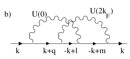
Figure 5: One of the self-energy diagrams for $U(0)\neq U(2k_{F})$. Momenta $q,l$ and $m$ are small compared to $k$.

It is then obvious that the overall factor for the diagram in Fig. 1b is $U(0)U(2k_{F})$. Process a) in Fig. 2 determines that part of the self-energy which is singular on the mass-shell and does not contribute to thermodynamics. The overall factor for that part is $U\left(0\right)^{2}$. Collecting all contributions, we find that

$$\Sigma_{R}^{\prime\prime}(\omega,T)=\frac{mU^{2}(0)}{16\pi^{3}v_{F}^{2}}~{}\left[\omega^{2}+(\pi T)^{2}\right]~{}\ln\frac{W}{|\omega-\epsilon_{k}|}$$

$$+\frac{m(U^{2}(0)+U^{2}(2k_{F})-U(0)U(2k_{F}))}{8\pi^{3}v_{F}^{2}}\left([(\pi T)^{2}+\omega^{2}]\ln\frac{{\bar{A}}}{T}-\omega^{2}~{}f\left(\frac{\omega}{\pi T}\right)\right),$$ (133)

where $A$ and ${\bar{A}}$ are constants, and the scaling function $f(x)$ is given by (44). The real part of the self-energy is given by

$$\Sigma_{R}^{\prime}(\omega)=-\frac{m(U^{2}(0)+U^{2}(2k_{F})-U(0)U(2k_{F}))}{16\pi^{2}v_{F}^{2}}\omega|\omega|g\left(\frac{\omega}{T}\right).$$ (134)

The limiting forms of the scaling function $g(x)$ are $g(\infty)=1$ and $g(x\ll 1)\approx 4log2/(x)$.

V.2 Spin and charge susceptibilities

The same consideration holds for the susceptibility–the very fact that all non-analytic contributions come from the vertices with near zero total momentum and transferred momentum either near zero or near $2k_{F}$ implies that for $U=U(q)$, an overall factor of $U^{2}$ is replaced either by $U^{2}(0)$ or $U^{2}(2k_{F})$, as in diagrams 1, 3, 6 and 7 in Fig.3, and by $U(0)U(2k_{F})$, as in diagrams 2, 4 and 5. With this substitution, we have, finally

$$\delta\chi_{1}(Q,T) = K(Q,T)(U^{2}(0)+U^{2}(2k_{F}));\delta\chi_{2}(Q,T)=-K(Q,T)U(0)U(2k_{F})$$

$$\delta\chi_{3}(Q,T) = K(Q,T)(U^{2}(2k_{F})-U^{2}(0));\delta\chi_{4}(Q,T)=K(Q,T)U(0)U(2k_{F});$$

$$\delta\chi_{5}(Q,T) = 0,~{}\delta\chi_{6}(Q,T)=-K(Q,T)(U^{2}(0)-U^{2}(2k_{F}));$$

$$\delta\chi_{7}(Q,T) = -K(Q,T)(U^{2}(0)+U^{2}(2k_{F})),$$ (135)

where $K(Q,0)$ and $K(0,T)$ are given by Eqs. (87) and (123), respectively:

$$K(Q,0)=\chi_{0}^{2D}~{}\frac{2}{3\pi}~{}\left(\frac{mU}{4\pi}\right)^{2}~{}\frac{|Q|}{k_{F}};~{}~{}K(0,T)=\chi_{0}^{2D}~{}\left(\frac{mU}{4\pi}\right)^{2}~{}\frac{T}{E_{F}}$$ (136)

where $\chi_{0}=m/\pi$. When both $Q$ and $T$ are nonzero, $K(Q,T)=K(Q,0){\tilde{g}}(v_{F}Q/T)$, where ${\tilde{g}}(x)$ is a scaling function subject to ${\tilde{g}}(x\gg 1)\propto 1/x$. However, we did not attempt to compute ${\tilde{g}}(x)$ at $x$ other than $x=0$ and $x=\infty$.

Collecting all contributions we find for the spin susceptibility

$$\delta\chi_{s}(Q,T)=2K(Q,T)U^{2}(2k_{F}).$$ (137)

As for the case $\ U=$const, the charge susceptibility is regular because all non-analytic corrections from individual diagrams cancel out.

Eqs. (133), (134), (136) and (137) are the central results of this paper.

While it is intuitively obvious that the momentum dependence of the susceptibility should only include $U(0)$ and $U(2k_{F})$, this intuition is based on the analysis of the self-energy but not the susceptibility itself. It is therefore worthwhile to demonstrate explicitly that non-analytic terms in the susceptibility do not depend on the momentum-averaged interaction. This is what we are going to do in the remainder of this Section.

To demonstrate that only $U(2k_{F})$ matters, consider one of the diagrams for which, as we claim, the non-analytic term scales as $U(0)U(2k_{F})$, i.e., diagrams 2, 4 and 5. Each of these diagrams has two interaction lines. Quite obviously, one of momentum transfers should be near zero. The issue is to prove that the other one is near $2k_{F}$. Consider for definiteness diagram 5. The net result for this diagram is zero, but this is a result of the cancelation between two contributions, $\delta\chi_{5}^{a}(Q)$ and $\delta\chi_{5}^{b}(Q)$, which differ in the choice of which of the two interactions carry small momentum. Consider one of the choices. We label the internal momenta in the diagram as $\mathbf{k}$, $\mathbf{k}+\mathbf{q}$, $\mathbf{k}+\mathbf{Q}$, $\mathbf{k}+\mathbf{q}+\mathbf{Q}$, $\mathbf{l}+\mathbf{q}/2$, $\mathbf{l}-\mathbf{q}/2$, where $Q$ is the external momentum, and introduce two angles $\theta_{1}$ and $\theta_{2}$ between $\mathbf{q}$ and $\mathbf{l}$ and between $\mathbf{q}$ and $\mathbf{k}$, respectively (cf. Fig.6).

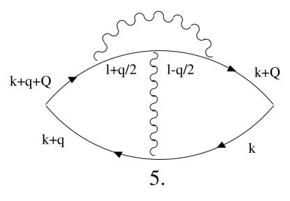
Figure 6: Another way of labeling momenta in $\delta\chi_{5}$.

The integration over $k$ and the corresponding frequency $\omega$ is straightforward (see Appendix E). Introducing then $q=r\cos\phi$ and $\Omega=r\sin\phi$, where $\Omega$ is the frequency associated with $q$, we integrate over $r$ and, after redefinition of the variables, obtain that the non-analytic, linear-in-$Q$ piece of diagram $5$ reduces to

$$\delta\chi_{5}^{a}(Q)=\chi_{0}\frac{m^{2}U(0)}{4\pi^{5}}\frac{|Q|}{k_{F}}~{}J,$$ (138)

where

$$J=\int_{0}^{\infty}dxx^{2}\int_{-\pi}^{\pi}\frac{d\theta_{1}}{x+i\cos\theta_{1}}~{}\int_{-\pi}^{\pi}\frac{d\theta_{2}}{(x+i\cos\theta_{2})^{4}}~{}U\left(2k_{F}\sin^{2}{\frac{\theta_{1}-\theta_{2}}{2}}\right).$$ (139)

For a constant interaction $U(q)=U$, we can integrate independently over $\theta_{1}$ and $\theta_{2}$, and then integrate over $x$, which gives $J=\pi^{2}/6$. The result for $\delta\chi_{5}^{a}(Q)$ then coincides with one of the two contributions to $\delta\chi_{5}(Q)$, as we discussed in Sec.IV.1.1. A relevant point here is that typical $\cos\theta_{1,2}$ are of order $x,$ whereas typical $x$ are of order 1. Hence $\theta_{1}-\theta_{2}\sim 1$, i.e., typical angles between two momenta are generic. This implies that the argument of $U(2k_{F}\sin^{2}(\theta_{1}-\theta_{2})/2)$ is just of the order of $k_{F}$ but not necessarily close to $2k_{F}.$

We now show that, in fact, only $\theta_{1}-\theta_{2}=\pm\pi$ matter. To see this, we introduce diagonal variables $a=(\theta_{1}+\theta_{2})/2$ and $b=(\theta_{1}-\theta_{2})/2$ and integrate first over $x$ and then over $a$. This integration is tedious but straightforward, and carrying it out we obtain, after some algebra,

$$J=-\int_{0}^{\pi/2}dbU(2k_{F}\sin^{2}b)\mbox{Re}\left[S(b)+S(\pi-b)\right],$$ (140)

where

$$S(b)=\left(\frac{4}{3}+\frac{\cos 2b}{\sin^{4}b}\right)\ln{\cos}2b\left(\frac{1}{\sin 2b-i\delta}-\frac{1}{\sin 2b+i\delta}\right).$$ (141)

Then

$$J=i\delta\mbox{Im}\int_{0}^{\pi}dz\ln\cos z\sin^{2}z{+}\delta{{}^{2}}\left(\frac{4}{3}+\frac{\cos z}{(\sin z/2)^{4}}\right)U(2k_{F}(\sin z/2)^{2})$$ (142)

The integral does not vanish due to divergences near $z=0$ and $z=\pi$. The divergence near $z=0$ does not contribute to the imaginary part of the integral, but the one near $z=\pi$ does contribute. Restricting $z$ near $\pi,$ we obtain

$$J=\frac{1}{3}U(2k_{F})\int_{0}^{\infty}\frac{dy\delta}{y^{2}+\delta^{2}}=\frac{\pi^{2}}{6}U(2k_{F}).$$ (143)

This consideration shows that although for a momentum-independent interaction we could evaluate $\delta\chi_{5}^{a}(Q)$ in a scheme in which the angular integrals were not restricted to a particular $\theta_{1}$ or $\theta_{2}$, the calculation performed in another way demonstrates that the whole integral comes only from the range where $\theta_{1}-\theta_{2}=\pm\pi$. For a momentum-dependent interaction, this implies that only $U(2k_{F})$ matters, precisely as we anticipated. Similar calculations can be repeated for other cross diagrams with the result that the overall factor is always $U(0)U(2k_{F})$.

The above consideration is another indication that the non-analyticities in the specific heat and spin susceptibility come from the two interaction vertices in which the transferred momentum is either near $0$ or $2k_{F}$, and simultaneously the total momentum for both vertices is near $2k_{F}$.

VI Conclusions

We now summarize the key results of the paper. We considered the universal corrections to the Fermi-liquid forms of the effective mass, specific heat, and spin and charge susceptibilities of the 2D Fermi liquid. We assumed that the Born approximation is valid, i.e., $mU(q)/4\pi\ll 1$, and performed calculations to second order in the interaction potential $U(q)$. We found that the corrections to the mass and specific heat are non-analytic and linear in $T$, and obtained for the first time the explicit results for these corrections. We next found that the corrections to the static spin susceptibility are also non-analytic and yield the $|Q|$-dependence of $\chi_{s}(Q,T=0)$ and $T$ dependence of $\chi_{s}(Q=0,T)$. We obtained for the first time the explicit expressions for the linear-in-$Q$ and linear-in-$T$ terms in the susceptibility. We found that the corrections to the charge susceptibility are all analytic. We also performed calculations in 3D and confirmed the results of BKV and others that the correction to $\chi_{s}(Q,T=0)$ scales as $Q^{2}\ln Q$, but the correction to $\chi_{s}(Q=0,T)$ scales as $T^{2}$ without a logarithmic prefactor.

We analyzed in detail the physical origin of the non-analytic corrections to the Fermi liquid and clarified the discrepancy between earlier papers. We argued that the non-analyticities in the fermionic self-energy and in $\chi_{s}(Q,T)$ are due to the non-analyticities in the dynamical particle-hole susceptibility. We argued that the non-analyticities in the fermionic self-energy and in $\chi_{s}(Q,0)$ are due to the non-analyticities in the dynamical two-particle response functions. We have shown that non-analytic terms in the self-energy and the spin susceptibility come from the processes which involve the scattering amplitude with a small momentum transfer and a small total momentum. We explicitly demonstrated that the non-analytic terms can be viewed equivalently as coming from either of the two non-analyticities in the dynamical particle-hole bubble–the one near $q=0$ and the other one near $q=2k_{F}$–or from the singularity in the dynamical particle-particle bubble near zero total momentum. We also demonstrated explicitly that the non-analytic terms in all diagrams for the susceptibility and the self-energy depend only on $U(0)$ and $U(2k_{F})$, but not on averaged interactions over the Fermi surface. Only under this condition, is there a substantial cancelation between different diagrams for the susceptibility. Due to these cancelations, the non-analytic correction to the spin susceptibility depends only on $U(2k_{F})$, but not on $U(0)$, and scales as $U^{2}(2k_{F})$. The non-analytic corrections to the effective mass and the spin susceptibility scale as $U^{2}(0)+U^{2}(2k_{F})-U(0)U(2k_{F})$.

The non-analytic $Q$ behavior of $\chi_{s}(Q,T=0)$ obtained in both 3D and 2D questioned the validity of the Hertz-Millis-Moriya phenomenological theory of quantum phase transitions. This theory assumes a regular $q^{2}$-expansion of the spin susceptibility. Indeed, extending the results for $\chi_{s}(Q,T)$ to the critical region one obtains a rather complex quantum critical behavior BK , which is very different from the Hertz-Millis-Moriya theory. We caution, however, that the non-analytic behavior of $\chi_{s}(Q,T)$ was obtained within the Born approximation, when fermions behave as sharp quasiparticles. Near a magnetic transition, the fermionic self-energy is large, and destroys the coherent Fermi-liquid behavior beginning at a frequency which vanishes at the quantum critical point. In this situation, the second-order perturbation theory is unreliable. The issue whether non-analytic corrections to the static $\chi_{s}(Q,T)$ survive at criticality is now under consideration and we refrain from further speculations on this matter.

We acknowledge stimulating discussions with A. Abanov, I. Aleiner, B. Altshuler, D. Belitz, S. DasSarma, A. Finkelstein, A. Millis, M. Norman, C. Pepin, A. Rosch, J. Rech, M. Reizer, and Q. Si. We also thank M. Mar’enko for bringing Ref.marenko to our attention and G. Martin for critical reading of the manuscript.

The research has been supported by NSF DMR 9979749 (A. V. Ch.) and NSF DMR-0077825 (DLM).

Appendix A Mass-shell singularity

In this Appendix, we take a deeper look into the origin of the logarithmic divergence of the self-energy on the mass shell. To better understand where it comes from, we come back to the derivation of (30). Re-writing (30) as (31a) to logarithmic accuracy, we now argue that the two logarithmic terms in (31a) come from two different processes, as shown in Fig.7. In the first process (Fig.7a), all four momenta are close to each other, and in the second one (Fig.7b), the net momentum of the two incoming particles is close to zero, whereas the momenta of the outgoing particles are close to their initial values. In terms of the momentum transfers, both processes are of forward-scattering type.

Figure 7: Two processes contributing to the log-singularities in the self-energy.

To see this, we notice that for generic $\omega/\epsilon_{k}$, i.e., not too close to the mass shell, the logarithmic form of the self-energy is due to $1/Q$ behavior of the momentum integrand at $v_{F}Q\gg\Omega,\omega$. This $1/Q$ form in 2D results from the combination of two facts: (i) the polarization operator $\Pi(Q,\Omega)$ behaves as $\Omega/v_{F}Q$, and (ii) the imaginary part of the fermionic propagator, integrated over the angle $\theta$ between $Q$ and external momentum $k$, behaves as $1/Q$. The product of the two terms yields $\int QdQ/Q^{2}$ that gives rise to a logarithm. It is easy to make sure that for $v_{F}Q\gg\Omega$, typical values of $\theta$ are close to $\pm\pi/2$, the deviation from these values being of order $\left|\Omega\right|/v_{F}Q$. That means that the external momentum ($\mathbf{k)}$ and the internal (small) one ($\mathbf{Q)}$ (as labeled in Fig.1a) are nearly orthogonal to each other. The same reasoning also works for the polarization bubble. If the two internal momenta in that bubble are $\mathbf{p}$ and $\mathbf{p}+\mathbf{Q}$, then typical $\mathbf{p}$ and $\mathbf{Q}$ are also nearly orthogonal. Since both $\mathbf{k}$ and $\mathbf{p}$ are orthogonal to the same $\mathbf{Q}$, and both are confined to the near vicinity of the Fermi surface, they are either near each other, or near the opposite points of the Fermi surface. If $\mathbf{p}$ and $\mathbf{k}$ are close to each other, all three internal fermionic momenta in the second-order diagram are close to external $\mathbf{k}$, if $\mathbf{p}$ is close to $-\mathbf{k}$, out of three internal momenta one is close to $\mathbf{k}$, while the other two are close to $-\mathbf{k}$. These two regions of intermediate momenta give rise to two logarithms in (31a). The logarithm that diverges on the mass shell comes from a region where all momenta are close to $\mathbf{k}$. To see this, we recall that the actual divergence is the consequence of the fact that both the polarization bubble and the angle-averaged $G^{\prime\prime}(\mathbf{k}+\mathbf{Q},\omega+\Omega)$ at the mass shell possess square-root singularities in the form $1/\sqrt{(v_{F}Q)^{2}-(\Omega)^{2}}$ such that the product of the two gives $(v_{F}Q)^{2}-(\Omega)^{2})^{-1}$, and the momentum integral diverges. The square-root singularities come from near parallel $\mathbf{p}$ and $\mathbf{Q}$ and $\mathbf{k}$ and $\mathbf{Q}$, respectively. Obviously then, $\mathbf{k}$ and $\mathbf{p}$ are near parallel, i.e., they are located near the same point at the Fermi surface. With a little more effort, one can show that as $\omega$ approaches $\epsilon_{k}$, typical angles between $\mathbf{p}$ and $\mathbf{Q}$ and between $\mathbf{k}$ and $\mathbf{Q}$, both move from near $\pi/2$ (or $-\pi/2$) to near zero, but in such a way that $\mathbf{k}$ and $\mathbf{p}$ remain parallel. This once again confirms that the divergent logarithm comes from the process in Fig.7a (all internal momenta are close to $k$), while the “conventional”, non-divergent $\omega^{2}\ln\omega$-term comes from the process in Fig.7b.

The analysis can be extended to finite $T$, and the (anticipated) result is that $\Sigma_{1}^{\prime\prime}$ given by (41) comes from forward scattering, while $\Sigma_{2}^{\prime\prime}$ given by (42) comes from back scattering.

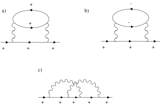
Figure 8: Non-trivial diagrams for the self-energy in 1D. $\pm$ denotes the propagator of a right/left moving fermion.

It is interesting follow the same arguments for $D=1.$ In this case, processes in Fig.7 acquire even simpler physical meanings: process a) is forward scattering of fermions of the same chirality, e.g., two right-moving fermions scatter into two right-moving ones, whereas process b) is forward scattering of fermions of opposite chirality, e.g., a right-moving fermion scatters at a left-moving one so that their respective chiralities are conserved. In the g-ology notations, vertex a) is $g_{2}$ and vertex b) is $g_{4}$ emery . In the Luttinger model, when only forward scattering is taken into account, the self-energy of, e.g., right-moving fermions is represented by the set of diagrams shown in Fig.8 DL , where $\pm$ denotes propagators of right/left moving species

$$G_{\pm}\left(k,\omega\right)=\frac{1}{i\omega-\epsilon_{k}^{\pm}},\text{ }\epsilon_{k}^{\pm}=v_{F}\left(k\mp k_{F}\right).$$ (144)

Diagrams a) and c) contain two vertices of type a) from Fig.7 whereas diagram b) contain vertices of type b) from Fig.7. The imaginary parts of the retarded polarization bubbles for right- and left-moving fermions for $\left|Q\right|\rightarrow 0$ are given by

$$\Pi_{R\pm}^{{}^{\prime\prime}}=\frac{Q}{2}\delta\left(\Omega\mp v_{F}Q\right).$$ (145)

The delta-function form of $\Pi_{R\pm}^{{}^{\prime\prime}}$ is due to the fact that in 1D and for $\left|Q\right|\rightarrow 0$ the particle-hole continuum shrinks to two lines in the $\left(\Omega,Q\right)$ plane described by $\Omega=v_{F}\left|Q\right|.$ The combination of the diagrams a) and c) in Fig.8 yields for the imaginary part of the self-energy

$$\left[\Sigma_{R+}^{\prime\prime}\left(\mathbf{k},\omega\right)\right]_{a)+c)}=\frac{U^{2}}{8\pi v_{F}^{2}}\omega^{2}\delta\left(\omega-\epsilon_{k}^{+}\right),$$ (146)

We see that $\Sigma_{R+}^{\prime\prime}$ given by (146), which is a 1D analog of our $\Sigma_{2}^{\prime\prime}$ from(31c), is very singular on the mass shell but vanishes outside the mass shell. At the same time, diagram b) in Fig.8 yields

$$\left[\Sigma_{R+}^{\prime\prime}\left(\mathbf{k},\omega\right)\right]_{b)}=\left\{\begin{array}[]{l}\frac{U^{2}}{2\pi v_{F}^{2}}\left(\left|\omega\right|-\left|\epsilon_{k}^{+}\right|\right),\text{ for }|\omega|>\left|\epsilon_{k}^{+}\right|;\\ 0,\text{ otherwise.}\end{array}\right..$$

This self-energy vanishes on the mass shell, but for a generic $\omega/\epsilon_{k}$ it yields $\left[\Sigma_{R+}^{\prime\prime}\left(k,\omega\right)\right]_{b)}\propto\left|\omega\right|$. This $|\omega|$ dependence obviously implies that Fermi-liquid behavior is in danger.

Which of the two terms is actually relevant? In 1D, the answer is well known: the summation of infinite series of the diagrams yields the non-Fermi-liquid behavior, and the resulting state–the Luttinger liquid–is free of singularities on the mass shell. This implies that the mass shell singularity of Eq.(146) is completely eliminated by the re-summation of diagrams to all orders in the interaction. This can be shown explicitly either via Ward identities or using the bosonization bosonization . Furthermore, the exact solution of the model with only type a) scattering (“$g_{4}$ -model”) yields a free-Fermi-gas behavior with a renormalized Fermi velocity, i.e., no mass-shell singularity. This all implies that the mass shell singularity found in the second-order self-energy diagram in 1D is an artificial one and is eliminated by higher order diagrams.

The same elimination of the mass shell singularity holds in 2D, as we now demonstrate. Indeed, as we mentioned before, the logarithmic divergence in (31a) at $\omega=\epsilon_{k}$ is the consequence of the matching of the two square-root singularities: one resulting from the angular integration of the fermionic Green’s function, and another one being the $1/\sqrt{(v_{F}Q)^{2}-\Omega^{2}}$ singularity in $\Pi_{R}^{\prime\prime}\left(Q,\Omega\right)$. Suppose now that the interaction gets renormalized (screened) by higher-order terms in $U$  so that $U\rightarrow U(Q,\Omega)$. The combination $U^{2}\Pi_{R}^{\prime\prime}\left(Q,\Omega\right)$ in (25) is now replaced by $U_{R}^{\prime\prime}(Q,\Omega).$ In the RPA approximation (which is not a controllable one for a short-range interaction),

$$U_{R}^{\prime\prime}\left(Q,\Omega\right)=\frac{U^{2}\Pi_{R}^{\prime\prime}\left(\Omega,Q\right)}{\left[1+U\Pi_{R}^{\prime}\left(Q,\Omega\right)\right]^{2}+\left[U\Pi_{R}^{\prime\prime}\left(\Omega,Q\right)\right]^{2}}$$ (147)

$$= \frac{2\pi}{m}\tilde{U}^{2}~{}\Omega~{}\frac{\sqrt{(v_{F}Q)^{2}-\Omega^{2}}\theta\left(v_{F}Q-\left|\Omega\right|\right)}{(1+\tilde{U})^{2}\left[(v_{F}Q)^{2}-\Omega^{2}\right]+\tilde{U}^{2}\Omega^{2}},$$

where $\tilde{U}\equiv mU/2\pi.$ Obviously, $U_{R}^{\prime\prime}$ now vanishes at $Q=\left|\Omega\right|/v_{F}$, and the divergence is eliminated. At the same time, the logarithmic dependence on $\Omega$ in (28), and hence the $\omega^{2}\ln\omega$ form of the self-energy, survive as they come from typical $\Omega\sim v_{F}Q$ for which $\Pi_{R}^{\prime}(Q,\Omega)$ and $\Pi_{R}^{\prime\prime}(Q,\Omega)$ are of the same order, and hence the screened interaction is of the order of the bare one. Note that this reasoning is also valid for the Coulomb interaction, for which the RPA approximation is asymptotically exact in the high-density limit.

Another argument that the mass-shell singularity is artificial is that it is eliminated, already at the second order of interaction, if one takes into account the curvature of the fermionic dispersion. Indeed, in obtaining (30), we linearized the fermionic dispersion near the Fermi surface, i.e., approximated $\epsilon_{k+q}$ by $\epsilon_{k}+v_{F}q\cos\theta$. Using the full quadratic dispersion, we obtain, instead of (29)

$$\Sigma_{R}^{\prime\prime}(\mathbf{k},\omega)=\frac{mU^{2}}{8\pi^{3}v_{F}^{2}}\int_{0}^{\omega}d\Omega~{}\Omega~{}\ln\frac{W^{2}}{\epsilon_{k}-\omega}][2\Omega-\omega+\epsilon_{k}]+\Delta\left(\omega,\Omega\right)|~{},$$ (148)

where

$$\Delta\left(\omega,\Omega\right)=\frac{\Omega^{2}}{2E_{F}}~{}\left(3\omega-\epsilon_{k}-\Omega\right)$$ (149)

and where, for the sake of definiteness, we assumed $\omega>0$. On the mass shell, $\omega=\epsilon_{k}$, the integration over $\Omega$ yields a finite result

$$\Sigma_{R}^{\prime\prime}(\mathbf{k},\omega)|_{\omega=\epsilon_{k}}=\frac{3U^{2}m}{16\pi^{3}v_{F}^{2}}\omega^{2}\ln\frac{W}{\left|\omega\right|}.$$ (150)

The crossover between Eqs.(30) and (150) occurs when, inside the log in Eq.(30), $\Delta\left(\omega,\Omega\right)$ becomes comparable to the other term in the denominator, i.e., when

$$\left|\omega-\epsilon_{k}\right|\sim\omega^{2}/W.$$ (151)

For $\left|\omega-\epsilon_{k}\right|\gg\omega^{2}/W,$ the leading asymptotic behavior of $\Sigma_{R}^{\prime\prime}(\mathbf{k},\omega)$ is given by (30) and for $\left|\omega-\epsilon_{k}\right|\ll\omega^{2}/W$ it is given by (150). A general formula which interpolates between the two limiting cases might, in principle, be obtained but we do not dwell on this here. Notice that $\Sigma_{R}^{\prime\prime}(\mathbf{k},\omega)$ on the mass shell is by a factor of 3/2 bigger than its value on the Fermi surface, which means that, for fixed $\omega,$ the slope of $\Sigma_{R}^{\prime\prime}(\mathbf{k},\omega)$ as function of $\epsilon_{k}$ becomes steeper as the mass shell is approached.

The same result can be also obtained by calculating the quasiparticle lifetime for $T=0$ which, by definition, is taken directly on the mass shell. For $D=2,$ the Fermi Golden Rule gives

$$1/\tau\left(\omega\right)=\frac{U^{2}m}{8\pi^{3}}\int_{0}^{\omega}d\Omega\int_{-\Omega}^{0}d\omega^{\prime}\int^{W/v_{F}}dQQ\int d\theta\int d\theta^{\prime}\delta\left(\Omega-\varepsilon_{\mathbf{k}}+\varepsilon_{\mathbf{k-Q}}\right)\delta\left(\Omega-\varepsilon_{\mathbf{p+Q}}+\varepsilon_{\mathbf{p}}\right),$$ (152)

where $\varepsilon=\epsilon_{\mathbf{k}}$ ,$\omega^{\prime}=\epsilon_{\mathbf{p}}$,  and $\theta$,$\theta^{\prime}$ are the angles between $\mathbf{k}$ and $\mathbf{q}$ and $\mathbf{p}$ and $\mathbf{q}$, respectively, and $W$ is the ultraviolet energy cutoff. For linearized dispersion the arguments of the first and second delta-functions in (152) reduce to $\Omega+v_{F}Q\cos\theta,\Omega-v_{F}Q\cos\theta^{\prime},$ respectively. Each of the angular integrations yields a factor of $2/\sqrt{(v_{F}Q)^{2}-\Omega^{2}},$ and the integral over $Q$

$$A=\int_{|\Omega|/v_{F}}^{W/v_{F}}dQQ\frac{1}{(v_{F}Q)^{2}-\Omega^{2}}$$ (153)

diverges logarithmically at the lower limit. To regularize the singularity, one must to keep the higher-order terms in $\varepsilon_{\mathbf{k-Q}}$ and $\varepsilon_{\mathbf{p+Q}}$. On the mass shell,

$$\varepsilon_{\mathbf{k}}-\varepsilon_{\mathbf{k-Q}} = v_{F}Q\left(1+\frac{\omega}{2E_{F}}\right)\cos\theta-\frac{Q^{2}}{2m};$$ (154a)

$$\varepsilon_{\mathbf{p}}-\varepsilon_{\mathbf{p+Q}} = -v_{F}Q\left(1+\frac{\omega^{\prime}}{2E_{F}}\right)\cos\theta^{\prime}-\frac{Q^{2}}{2m}.$$ (154b)

Now the integral over $$Q$$ takes the form

$$A=\int^{W/v_{F}}dQQ\frac{1}{\sqrt{\left(v_{F}Q\right)^{2}-\Omega^{2}-\delta}}\frac{1}{\sqrt{\left(v_{F}Q\right)^{2}-\Omega^{2}+\delta^{\prime}}},$$ (155)

where

$$\delta = \Omega\left(v_{F}Q\frac{\omega}{E_{F}}+\frac{Q^{2}}{m}\right)$$ (156a)

$$\delta^{\prime} = \Omega\left(v_{F}Q\frac{\omega^{\prime}}{E_{F}}+\frac{Q^{2}}{m}\right)$$ (156b)

The lower limit in the integral is such that the arguments of the square roots are positive. The momentum integral is controlled by $$Q\sim|\Omega|/v_{F} Q |\Omega|/v_{F}$$. To logarithmic accuracy, one can then just replace by in (156a,156b). After this replacement, the momentum integration can be easily performed and gives

$$A=\frac{1}{2v_{F}^{2}}\ln\frac{E_{F}^{2}W}{\Omega^{2}\left(\omega+\omega^{\prime}\right)+\Omega^{3}}.$$ (157)

We next have to perform the frequency integration. It is easy to verify that, in the two integrals over frequency, the dominant contributions come from the regions $\Omega\sim\omega^{\prime}\sim\omega$. To logarithmic accuracy, one can then simplify $A$ to

$$\frac{3}{2v_{F}^{2}}\ln\frac{W}{\omega}.$$ (158)

We also used the fact that $E_{F}\sim W$. Substituting this into (152 and performing frequency integrations we obtain finally

$$\frac{1}{\tau\left(\omega\right)}=\frac{3U^{2}m}{8\pi^{3}v_{F}^{2}}\omega^{2}\ln\frac{W}{\omega}.$$ (159)

We see that $1/\tau(\omega)$ is finite–the only memory left about the mass-shell singularity for the linearized spectrum is the enhanced numerical prefactor. Identifying $1/\tau$ with $2\Sigma_{R}^{\prime\prime}$, we see that the results for $1/\tau$ and $\Sigma^{\prime\prime}(\omega=\epsilon_{k})$ coincide, as indeed they should.

Appendix B Polarization bubble near $2k_{F}$

In this Appendix, we show that the computation of a non-analytic piece in the particle-hole bubble at $Q\approx 2k_{F}$ can be always performed in such a way that the dominant contribution comes from fermions near the Fermi surface and with nearly antiparallel momenta $\pm\mathbf{Q}/2$. We do this in two ways. First, we compute $\Pi_{ph}(Q,\Omega_{m})$ explicitly and check where the non-analyticity comes from. Second, we compute $\Pi_{ph}(Q,\Omega_{m})$ by linearizing the dispersion of fermions, forming the polarization bubble, near $\pm\mathbf{Q}/2$ and show that the non-analyticity in $\Pi_{ph}(Q,\Omega_{m})$ comes from the lower limit of momentum integration and therefore does not depend on the upper cutoff imposed by the linearization procedure.

B.1 Explicit computation

Consider first $T=0$. Labeling the momenta of internal fermionic lines in the polarization bubble as $\mathbf{p}\pm\mathbf{Q}/2$ and for $T=0$, we obtain in Matsubara frequencies

$$\Pi(Q,\Omega_{m})=-\int\frac{d^{2}pd\omega}{(2\pi)^{3}}G(\mathbf{p}+\frac{\mathbf{Q}}{2},\omega_{n}+\Omega_{m})~{}G(\mathbf{p}-\frac{\mathbf{Q}}{2},\omega_{n}).$$ (160)

For a circular Fermi surface

$$\epsilon_{\mathbf{p}\pm\mathbf{Q}/2}=\frac{p^{2}-k_{F}^{2}}{2m}\pm\frac{pQ\cos\theta}{2m}+\frac{Q^{2}}{8m}.$$ (161)

Substituting (161) into (160) and integrating over frequency and then over $p,$ we obtain for $Q<2k_{F}$

$$\Pi(Q,\Omega_{m})=\frac{m}{2\pi}\left(1-2\frac{m\Omega_{m}}{\pi Q^{2}}\int_{0}^{\pi/2}\frac{d\theta}{\cos^{2}\theta}\left[\arctan\frac{p_{1}}{m\Omega_{m}}-\arctan\frac{p_{2}}{m\Omega_{m}}\right]\right),$$ (162)

where

$$p_{1,2}=Q\cos{\theta}\sqrt{k_{F}^{2}-\frac{Q^{2}}{4}\sin^{2}\theta}\pm\frac{1}{2}Q^{2}\cos^{2}\theta.$$ (163)

For $Q=2k_{F}$, we have $p_{1}=4k_{F}^{2}\cos^{2}\theta,~{}p_{2}=0$, and (162) reduces to

$$\Pi(Q,\Omega_{m})=\frac{m}{2\pi}\left(1-2\frac{m\Omega_{m}}{\pi Q^{2}}\int_{0}^{\pi/2}\frac{d\theta}{\cos^{2}\theta}\arctan\frac{4k_{F}^{2}\cos^{2}\theta}{m\Omega_{m}}\right)=\frac{m}{2\pi}\left(1-\frac{1}{2}\left(\frac{|\Omega_{m}|}{E_{F}}\right)^{1/2}\right).$$ (164)

It is easy to see that the integral comes from $\cos^{2}\theta\sim|\Omega|/E_{F}$, i.e. typical $\mathbf{p}$ are nearly orthogonal to $\mathbf{Q}$. Furthermore, in the integral over $p$, typical $p$ were of order $Q\cos\theta$. Hence typical $p$ are of order $\sqrt{m|\Omega_{m}|}$, i.e. at vanishing $\Omega$, the integration is indeed confined to internal momenta which nearly coincide with $\pm\mathbf{Q/2}$.

The same reasoning is valid also for $Q$ in a narrow range near $2k_{F}$. For $Q\leq 2k_{F}$, Eq. (164) can be re-written as

$$\Pi(Q,\Omega_{m})=\frac{m}{2\pi}\left(1-2\frac{m\Omega_{m}}{\pi Q^{2}}\int_{0}^{\pi/2}\frac{d\theta}{\cos^{2}\theta}\arctan\frac{Q^{2}\cos^{2}\theta}{(m\Omega_{m})(1-Q^{2}\cos^{2}\theta\epsilon^{2})}\right),$$ (165)

where $\epsilon^{2}=(Q^{2}/4-k_{F}^{2})/m|\Omega_{m}|$. Assuming that the integral is dominated by $\theta$ near $\pi/2$ and expanding $\theta$ to linear order near $\pi/2$, we obtain after simple manipulations

$$\Pi(Q,\Omega_{m})=\frac{m}{2\pi}\left(1-\frac{(m|\Omega_{m}|)^{1/2}}{\pi k_{F}}\int_{0}^{\infty}dz\arctan\frac{1}{z^{2}-\epsilon^{2}}\right).$$ (166)

We see that the integral is convergent, i.e., the linearization of $\cos\theta$ near $\pi/2$ does not lead to cutoff-dependent integrals. This implies that the non-analytic piece in the polarization operator comes from typically small $\cos\theta$ and hence from typically small internal $p\propto\cos\theta$. Evaluating the integral over $z$ in (166), we obtain

$$\Pi(Q,\Omega_{m})=\frac{m}{2\pi}\left(1-\frac{1}{2}~{}\left(\frac{|\Omega_{m}|}{E_{F}}\right)^{1/2}~{}\left(\frac{v_{F}{\tilde{Q}}}{|\Omega_{m}|}+\sqrt{1+\left(\frac{v_{F}{\tilde{Q}}}{|\Omega_{m}|}\right)^{2}}\right)^{1/2}\right).$$ (167)

where ${\tilde{Q}}=Q-2k_{F}$. This is the result that we cited in the text (Eq. (15)).

For $Q>2k_{F}$, i.e., ${\tilde{Q}}>0$, the calculations proceed in the same way. Integrating over $p$ and over $\omega$ and again expanding to linear order near $\theta=\pi/2$ we obtain after straightforward manipulations

$$\Pi(Q,\Omega_{m})=\frac{m}{2\pi}\left(1-\left(\frac{\tilde{Q}}{k_{F}}\right)^{1/2}-\frac{1}{\pi\sqrt{2}}~{}\left(\frac{|\Omega_{m}|}{E_{F}}\right)^{1/2}\int_{0}^{1/2\epsilon}dz\arctan\frac{(1-4\epsilon^{2}z^{2})^{1/2}}{z^{2}+\epsilon^{2}}\right).$$ (168)

Evaluating the integral we find that the result reduces to Eq. (167).

B.2 Another way of calculating $\Pi(Q\approx 2k_{F},\Omega_{m})$

For completeness, we also compute the non-analytic part in $\Pi(Q,\Omega_{m})$ near $2k_{F}$ by explicitly restricting the integral over $p$ in (160) to small $p$ and assuming that $\mathbf{p}$ is nearly orthogonal to $\mathbf{Q}$. This calculation shows in a more direct way that typical values $p$ are indeed small. To avoid lengthy calculations, we assume that $Q=2k_{F}$ and aim at reproducing the $\sqrt{\Omega_{m}}$ non-analyticity. For $Q=2k_{F}$, the energies on the internal fermionic lines are $\epsilon_{k_{F}\hat{n}+\mathbf{p}}$ and $\epsilon_{-k_{F}\hat{n}+\mathbf{p}}$. Introducing $x=v_{F}p$ and $\gamma=1/(2mv_{F}^{2})=1/(4E_{F})$, expanding $\cos\theta\approx\tilde{\theta}$, where $\tilde{\theta}=\pi/2-\theta$ and substituting into (160), we obtain

$$\Pi(2k_{F},\Omega_{m})=\frac{1}{4\pi^{3}v_{F}^{2}}\int_{-\infty}^{\infty}d\tilde{\theta}\int_{-\infty}^{\infty}d\omega\int_{0}^{\infty}dx~{}\frac{x}{(x\tilde{\theta}+\gamma x^{2}-i\omega_{n})~{}(x\tilde{\theta}-\gamma x^{2}+i(\omega_{n}+\Omega_{m}))}.$$ (169)

Introducing $y=x\tilde{\theta}$ and integrating over $y,$ we obtain after simple manipulations with variables

$$\Pi(2k_{F},\Omega_{m})=\frac{1}{2\pi^{2}v_{F}^{2}}\int_{0}^{\infty}dx\int_{|\Omega_{m}|}^{\infty}\frac{zdz}{z^{2}+4\gamma^{2}x^{4}}.$$ (170)

The integration is elementary and yields

$$\Pi(2k_{F},\Omega)=\frac{1}{8\pi v_{F}^{2}\sqrt{\gamma}}\int_{|\Omega_{m}|}^{\infty}\frac{dz}{\sqrt{z}}.$$ (171)

The divergence of the integral at the upper limit simply reflects that a constant term in the polarization bubble cannot be reproduced this way. However, the lower limit of the integral over $z$ yields a universal and non-analytic contribution to $\Pi(2k_{F},\Omega_{m})$ of the form

$$\Pi_{\text{sing}}(2k_{F},\Omega_{m})=-\frac{1}{4\pi v_{F}^{2}}\left(\frac{|\Omega_{m}|}{\gamma}\right)^{1/2}=-\frac{m}{4\pi}\left(\frac{|\Omega_{m}|}{E_{F}}\right)^{1/2}.$$ (172)

This coincides with Eq. (167). It is essential that this result does not depend on the upper limit, and hence typical internal momenta scale with external $\Omega$. This obviously implies that typical values of $p$ are indeed small.

B.3 Finite temperature

At finite $T$, a sharp $\sqrt{Q-2k_{F}}$ non-analyticity in the static polarization operator is softened in qualitatively the same way as it is softened by a finite $\Omega_{m}$ at $T=0$. In general,

$$\Pi(Q,\Omega_{m},T)=\frac{m}{2\pi}\left(1-\left(\frac{T}{E_{F}}\right)^{1/2}\Phi\left(\frac{v_{F}|Q-2k_{F}|}{T},\frac{\Omega_{m}}{T}\right)\right).$$ (173)

We could not find a simple analytical expression for the scaling function $\Phi(x,y)$ at arbitrary values of its arguments. At $Q=2k_{F}$ and $\Omega=0$, $\Phi(0,0)\approx 0.339$.

Appendix C Equivalence of $q=0$ and $q=2k_{F}$ contributions to the self-energy

In this appendix, we explicitly compute the contribution to the self-energy from the $2k_{F}$ non-analyticity in the particle-hole bubble, and show that it is equal to the backscattering part of the self-energy from the $q=0$ non-analyticity. We will also show that the non-analytic self-energy can be equally viewed as coming from the singularity in the particle-particle channel at zero total momentum and frequency.

C.1 $2k_{F}$ part of the self-energy from the particle-hole channel

Since our goal is to verify a general reasoning that $q=0$ and $2k_{F}$ contributions to $\Sigma(k,\omega)$ are equal, we focus on the case $T=\epsilon_{k}=0$, compute the $2k_{F}$ part of the self-energy in Matsubara frequencies and compare the prefactor for $\omega_{n}\ln|\omega_{n}|$ term with $1/2$ of that in Eq. (37).

For a contact interaction, the second-order self-energy is

$$\Sigma(k,\omega_{n})=-U^{2}\int\int\frac{d^{2}qd\Omega_{m}}{(2\pi)^{3}}~{}G_{0}(\mathbf{k}+\mathbf{q},\omega_{n}+\Omega_{m})~{}\Pi_{ph}(q,\Omega_{m}).$$ (174)

Assuming $q=2k_{F}+\tilde{q}$, where $\tilde{q}$ is small, we expand $\epsilon_{k+q}$ as $\epsilon_{\mathbf{k+q}}=-\epsilon_{k}+v_{F}\tilde{q}+2v_{F}k_{F}(1+\cos\theta)$, where $\theta$ is the angle between $\mathbf{k}$ and $\mathbf{q}$. As we already discussed in Appendix B, only $\theta$ near $\theta=\pi$ matter (i.e., typical $\mathbf{q}$ is nearly antiparallel to $\mathbf{k}$), hence we can further approximate $\epsilon_{\mathbf{k+q}}$ as

$$\epsilon_{\mathbf{k+q}}\approx-\epsilon_{k}+v_{F}\tilde{q}+v_{F}k_{F}\tilde{\theta}^{2},$$ (175)

where ${\tilde{\theta}}=\pi-\theta$. Substituting (175) into (160), we obtain, setting $\epsilon_{k}=0$,

$$\Sigma(\omega_{n})=\frac{2U^{2}k_{F}}{(2\pi)^{3}}~{}\int_{-\infty}^{\infty}d\tilde{q}~{}d\Omega_{m}~{}\int_{0}^{\infty}d{\tilde{\theta}}~{}\frac{1}{v_{F}\tilde{q}+v_{F}k_{F}{\tilde{\theta}}^{2}-i(\omega_{n}+\Omega_{m})}~{}\Pi_{ph}(\tilde{q},\Omega_{m}),$$ (176)

where $\Pi_{ph}(\tilde{q},\Omega_{m})$ is given by (15).

As an exercise, consider first a model case where $\Pi_{ph}(\tilde{q},\Omega_{m})$ is static. To ensure convergence, we assume that the static behavior holds for $\Omega_{m}\ll\Omega_{0},$ where $\Omega_{0}$ is some ultraviolet cutoff (of order bandwidth), and for larger $\Omega_{m}$, $\Pi_{ph}({\tilde{q}},\Omega_{m})$ rapidly falls off. The angular integration in (174) reduces the range of integration over $\Omega_{m}$ to $-\omega_{n}\leq\Omega_{m}\leq\omega_{n},$ hence at the smallest $\omega_{n}$, $\Sigma\propto\omega_{n}$. This accounts for the conventional mass renormalization. We now show that there are no non-analytic corrections to $\Sigma$ in this model. A static $\Pi_{ph}(\tilde{q},0)$ is non-analytic only for $\tilde{q}>0$, where $\Pi_{ph}(\tilde{q},\Omega_{m})=(m/2\pi)(1-(\tilde{q}/k_{F})^{1/2})$. Substituting non-analytic part of the polarization bubble into (164) introducing $\tilde{\theta}=\sqrt{r/v_{F}k_{F}}\cos\phi,~{}\sqrt{\tilde{q}}=\sqrt{r/v_{F}}\sin\phi$, and integrating over $\phi$, we obtain for a potentially non-analytic part of the self-energy

$$\Sigma(\omega)=-\frac{mU^{2}}{32\pi^{3}v_{F}^{2}}~{}\int_{-\infty}^{\infty}d\Omega_{m}~{}\int_{0}^{\infty}\frac{rdr}{r-i(\omega_{n}+\Omega_{m})}.$$ (177)

One can easily make sure that this integral yields a regular $\omega$ term (determined by high-energy states), but no universal $\omega^{2}\ln\omega$-term. This implies, as we mentioned several times in the text, that static $\Pi_{ph}(\tilde{q},0)$ does not give rise to a non-analyticity in the fermionic self-energy.

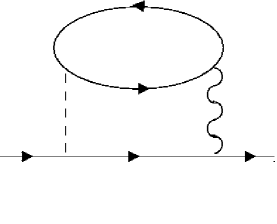
Figure 9: Hartree contribution to the self-energy for scattering at a Friedel oscillation.

It is instructive to distinguish this case from the impurity problem. If one of the interaction lines in Fig.1a is replaced by an impurity line, as shown in Fig. 9, the diagram in Fig. 1a transforms into the Hartree diagram describing the scattering of fermions by Friedel oscillations produced by impurities. In the ballistic limit, $\left|\omega_{n}\right|\tau\gg 1,$ it suffices to keep only a single impurity line connecting $G$ and $\Pi_{ph}$ and also neglect disorder in G. For delta-correlated disorder with amplitude $V$, the analytic expression for the diagram in Fig. 9 takes the form

$$\Sigma(k,\omega_{n})=-2UV\int\frac{d^{2}q}{(2\pi)^{3}}~{}G_{0}(\mathbf{k}+\mathbf{q},\omega_{n})~{}\Pi_{ph}(q,0).$$ (178)

The particle-hole bubble is still static, but in distinction to 174 we no longer have to perform a summation over frequencies. The non-analytic piece in $\Sigma(\omega)$ is then given by, instead of Eq.(165),

$$\Sigma(\omega_{n})=-\frac{mUV}{4\pi^{3}v_{F}^{2}}~{}~{}\int_{0}^{\infty}\frac{rdr}{r-i\omega_{n}}.$$ (179)

Due to the absence of the integral over $\Omega_{m},$ (177) does yield a universal contribution $\Sigma(\omega_{n})\propto-i\omega_{n}\ln\left(-i\omega_{n}\right)$ which comes from the lower limit of the integral over $r.$ Upon analytic continuation, one obtains $\Sigma_{R}^{\prime}\propto\omega\ln\left|\omega\right|$ and $\Sigma_{R}^{{}^{\prime\prime}}\left(\omega\right)\propto\left|\omega\right|.$ The linear in $\omega$ form of $\Sigma_{R}^{{}^{\prime\prime}}\left(\omega\right)$ is related to the Hartree part of the linear-in-$T$ term in the conductivity at finite $T$ zna .

We now come back to the electron-electron interaction, when a non-analytic-in-$\omega_{n}$ behavior of $\Sigma\left(\omega_{n}\right)$ can be obtained if the $\Omega_{m}-$ dependence is retained in $\Pi_{ph}(\tilde{q},\Omega_{m})$. As with any logarithmic singularity, typical $\tilde{q}$ should well exceed $\omega_{n}/v_{F}$. We will see that typical $\Omega_{m}$ are of order $\omega_{n}$. Typical values of $v_{F}\tilde{q}$ well exceed then typical values of $\Omega_{m}$, and one can expand $\Pi_{ph}(\tilde{q},\Omega_{m})$ in powers of $\Omega_{m}/v_{F}\tilde{q}$.  For $\tilde{q}>0$, the frequency expansion of $\Pi_{ph}(\tilde{q},\Omega_{m})$ starts at a constant and holds in even powers of $\Omega_{m}/v_{F}\tilde{q}$. We have already verified that the constant term does not give rise to an $\omega^{2}\ln\omega$-piece in $\Sigma(\omega)$. At $\tilde{q}<0$, however, the leading expansion term has the same $|\Omega_{m}|$ non-analyticity as the polarization operator near $q=0$. The non-analytic behavior in frequency is crucial as it prevents one from eliminating a low-energy non-analyticity by closing the integration contour in the integral over $\Omega_{m}$ over a distant semi-circle in a half-plane where the denominator in (164) has no poles.

Expanding $\Pi_{ph}(\tilde{q},\Omega_{m})$ at $\tilde{q}<0$ and $\Omega_{m}\ll v_{F}|{\tilde{q}}|$ , we find

$$\Pi_{ph}({\tilde{q}},\Omega_{m})=\frac{m}{2\pi}\left(1-\frac{|\Omega_{m}|}{2v_{F}(k_{F}|\tilde{q}|)^{1/2}}\right).$$ (180)

Substituting this result into Eq.(164) and keeping only potentially non-analytic piece, we obtain

$$\Sigma(\omega)=-\frac{2mU^{2}k_{F}}{(2\pi)^{4}}~{}\int_{-\infty}^{\infty}d\Omega_{m}~{}\int_{-\infty}^{0}d\tilde{q}~{}\int_{0}^{\infty}d\tilde{\theta}~{}\frac{1}{v_{F}\tilde{q}+v_{F}k_{F}\tilde{\theta}^{2}-i(\omega_{n}+\Omega_{m})}~{}\frac{|\Omega_{m}|}{v_{F}(k_{F}|\tilde{q}|)^{1/2}}.$$ (181)

Introducing $x^{2}=-v_{F}\tilde{q}~{}$and $y^{2}=v_{F}k_{F}\tilde{\theta}^{2}$ , we obtain from (181)

$$\Sigma(\omega)=-\frac{mU^{2}}{4\pi^{4}v_{F}^{2}}~{}\int_{-\infty}^{\infty}d\Omega_{m}~{}|\Omega_{m}|~{}\int_{0}^{\infty}\int_{0}^{\infty}\frac{dx~{}dy}{y^{2}-x^{2}-i(\omega_{n}+\Omega_{m})}.$$ (182)

Introducing further $y=\sqrt{r}\cos\phi/2,~{}x=\sqrt{r}\sin\phi/2$ and integrating over $\phi$ first, we obtain

$$\Sigma(\omega) = -\frac{mU^{2}}{8\pi^{4}v_{F}^{2}}~{}\int_{-\infty}^{\infty}d\Omega_{m}~{}|\Omega_{m}|~{}\int_{0}^{W}\frac{dr}{r}\int_{0}^{\pi}\frac{d\phi}{\cos\phi-i(\omega+\Omega)/r}$$ (183)

$$= -i\frac{mU^{2}}{8\pi^{3}v_{F}^{2}}~{}\int_{-\infty}^{\infty}d\Omega_{m}~{}|\Omega_{m}|~{}\text{sgn}(\omega_{n}+\Omega_{m})~{}\int_{0}^{W^{2}}\frac{dr}{(r^{2}+(\omega_{n}+\Omega_{m})^{2})^{1/2}}.$$

Evaluating the integral over $r$ with logarithmic accuracy and integrating finally over $\Omega_{m},$ we obtain

$$\Sigma(\omega)=-i\frac{mU^{2}}{16\pi^{3}v_{F}^{2}}~{}\omega_{n}^{2}\ln\frac{W^{2}}{\omega_{n}^{2}}.$$ (184)

This coincides with the half of Eq.(37) for $\epsilon_{k}=0.$

To further clarify this issue, we redo the calculation in a different way. Namely, we use the fact that for $\mathbf{Q}=-2\mathbf{k}+\mathbf{Q}^{\prime}$, and $Q^{\prime}$ small, the non-analytic part of the bubble $\Pi_{ph}(Q^{\prime},\Omega_{m})$ comes from the region of small $Q^{\prime\prime}$ in the following integral:

$$\Pi_{ph}(Q^{\prime},\Omega_{m})=-\int\int\frac{d^{2}Q^{\prime\prime}d\omega_{n}}{(2\pi)^{3}}~{}G_{\mathbf{k+Q}^{\prime\prime},\omega_{n}}~{}G_{-\mathbf{k+Q}^{\prime}\mathbf{+Q}^{{}^{\prime\prime}},\omega_{n}+\Omega_{m}}.$$ (185)

Now, we want to re-express the $2k_{F}$ contribution as an effective $Q=0$ contribution. To do this, we substitute (185) into (160) and change the order of the integrations over $Q^{\prime}$ and $Q^{{}^{\prime\prime}}$. The non-analytic “$2k_{F}$” piece in the self-energy then becomes

$$\Sigma(k,\omega_{n})=-U^{2}\int\int\frac{d^{2}Q^{\prime\prime}d\Omega_{m}}{(2\pi)^{3}}~{}G_{\mathbf{k+Q}^{\prime},\omega_{n}+\Omega_{m}}{\tilde{\Pi}}(Q^{\prime},\Omega_{m}),$$ (186)

where the effective particle hole-bubble

$${\tilde{\Pi}}(Q^{\prime\prime},\Omega_{m})=-\int\int\frac{d^{2}Q^{{}^{\prime\prime}}d\omega_{n}}{(2\pi)^{3}}~{}G_{-\mathbf{k+Q}^{\prime\prime},\omega_{n}}~{}G_{-\mathbf{k+Q}^{\prime}\mathbf{+Q}^{{}^{\prime\prime}},\omega_{n}+\Omega_{m}}.$$ (187)

This $\tilde{\Pi}$ is a part of the particle-hole polarization bubble at small momentum transfer, which comes from the integration over small $Q^{{}^{\prime\prime}}$. We now show that for $\Omega_{m}\ll v_{F}Q^{{}^{\prime\prime}}$, i.e., in the momentum/frequency range which yields the logarithm in the self-energy, the non-analytic part of ${\tilde{\Pi}}(Q,\Omega_{m})$ is a half of that in $\Pi(Q,\Omega_{m})$. This would again imply that the $2k_{F}$ contribution to the self-energy coincides with the (non-divergent) $\Sigma_{2}$ part of “$q=0$” contribution.

The calculation proceeds as follows. We set $\epsilon_{k}=0$ and write $\epsilon_{-\mathbf{k+Q}^{\prime}}=-x\cos\theta_{1}+\gamma x^{2}$ where $x=v_{F}Q^{\prime}$, $\gamma=(2mv_{F}^{2})^{-1}$, and $\theta_{1}$ is the angle between $\mathbf{k}$ and $\mathbf{Q}^{\prime}$. Similarly, $\epsilon_{-\mathbf{k+Q}^{\prime}}=-x\cos\theta_{1}-y\cos\theta_{2}+\gamma(x^{2}+y^{2}+2xy\cos(\theta_{1}-\theta_{2}))$, where $y=v_{F}Q$, and $\theta_{2}$ is the angle between $\mathbf{k}$ and $\mathbf{Q}$. As we said, we need to evaluate ${\tilde{\Pi}}$ for $\theta_{2}$ close to $\pm\pi/2$, and small $y$. We therefore neglect $y^{2}$ terms and set $\theta_{2}\approx\pi/2$ for definiteness. We assume and then verify that $\Omega/v_{F}Q$ term in the polarization operator comes from $\theta_{1}$ near $\pm\pi_{/}2$ and linearize $\cos\theta_{1}$ near these points. The integration over $\theta_{1}$ is then straightforward, and performing it we obtain that the integration over $\omega_{n}$ is confined to $-\Omega_{m}<\omega_{n}<0$ (for definiteness we assumed that $\Omega_{m}>0$). The result is

$${\tilde{\Pi}}(Q,\Omega_{m})=\frac{i\Omega_{m}}{4\pi^{2}v_{F}^{2}\gamma y}\int_{0}^{\infty}dp\left(\frac{1}{\cos\theta_{2}-2p-i\Omega_{m}}+\frac{1}{\cos\theta_{2}+2p-i\Omega_{m}}\right),$$ (188)

where we introduced $p=\gamma x$. The integration over $p$ is straightforward, and for small $\Omega_{m}$ and $\cos\theta_{2}$ the integral over $dp$ yields $i\pi/2$. Substituting this into (188) we obtain

$${\tilde{\Pi}}(Q,\Omega_{m})=\frac{1}{2}~{}\frac{m}{2\pi}\frac{\Omega_{m}}{v_{F}Q}.$$ (189)

It is essential that the momentum integral is confined to small $p=Q^{\prime}/k_{F}$ (typical $p\sim\cos\theta_{2}\sim\Omega_{m}/v_{F}Q$), and hence we are really restricting our momentum integral to small $Q^{\prime}$. Comparing (189) and (13) we see that, as we expected, (189) is a half of a non-analytic part of $\Pi(Q,\Omega_{m})$ at $\Omega_{m}\ll v_{F}Q$. Another half obviously comes from the region of large $Q^{\prime}$, which cannot be re-expressed as a “$2k_{F}$ contribution.”

C.2 An alternative computation of the self-energy, via $\Pi_{pp}(q,\Omega)$

We discussed in the text that the second-order self-energy can be equivalently presented as a convolution of the fermionic Green’s function and the particle-particle bubble

$$\Sigma(\omega_{n})=-U^{2}\int\int\frac{d^{2}qd\Omega_{m}}{(2\pi)^{3}}~{}G_{0}(-k_{F}\hat{n}+\mathbf{q},-\omega_{n}+\Omega_{m})~{}\Pi_{pp}(q,\Omega_{m}),$$ (190)

where $\Pi_{pp}(q,\Omega_{m})=(m/2\pi)\ln\left[B/\left(|\Omega_{m}|+\sqrt{\Omega_{m}+(v_{F}q)^{2}}\right)\right]$. Substituting this $\Pi_{pp}$ into the self-energy and expanding $\epsilon_{-k_{F}\hat{n}+\mathbf{q}}$ as $-v_{F}q\cos\theta$, we obtain for $\epsilon_{k}=0$

$$\Sigma(\omega_{n})=-\frac{mU^{2}}{8\pi^{4}v_{F}^{2}}~{}\int_{-\infty}^{\infty}d\Omega_{m}\int_{0}^{\pi}d\theta\int_{0}^{W}dx\frac{x}{x\cos\theta+i(\Omega_{m}-\omega_{n})}~{}\ln\frac{B}{|\Omega_{m}|+\sqrt{\Omega_{m}+x^{2}}}.$$ (191)

Assuming, as before, that typical $\Omega_{m}$ are of order $\omega_{n}$, while typical $x=v_{F}q$ are much larger, we can further expand under the logarithm and obtain

$$\Sigma(\omega_{n})=\frac{mU^{2}}{8\pi^{4}v_{F}^{2}}~{}\int_{-\infty}^{\infty}d\Omega_{m}|\Omega_{m}|~{}\int_{0}^{\pi}d\theta\int_{0}^{W}dx\frac{1}{x\cos\theta+i(\Omega_{m}-\omega_{n})}.$$ (192)

The integration over $\theta$ yields

$$\Sigma(\omega_{n})=i\frac{mU^{2}}{8\pi^{3}v_{F}^{2}}~{}\int_{-\infty}^{\infty}d\Omega_{m}|\Omega_{m}|~{}\text{sgn}(\Omega_{m}-\omega_{n})~{}\int_{0}^{W}dx\frac{1}{\sqrt{x^{2}+(\Omega_{m}-\omega_{n})^{2}}}.$$ (193)

Evaluating the integral over $x$ to logarithmic accuracy, we finally obtain

$$\Sigma(\omega_{n})=-i\frac{mU^{2}}{16\pi^{3}v_{F}^{2}}\omega_{n}\ln\frac{W^{2}}{\omega_{n}}.$$ (194)

This coincides precisely with Eq.(170).

Appendix D Evaluation of $\Sigma_{R}^{\prime}(\omega,\epsilon_{k})$ on the mass shell

In this Appendix, we present the calculation of the real part of the fermionic self-energy on the mass shell. We will be only interested in the non-analytic piece of the self-energy. The non-analytic part of $\Sigma_{R}^{\prime}(\omega)$ is simply twice of $\Sigma_{2}^{\prime}(\omega),$ where, according to Eq. (56), $\Sigma_{2}^{\prime}(\omega)$ can be written as

$$\Sigma_{2}^{\prime}(\omega)=-\frac{mU^{2}}{16\pi^{4}v_{F}^{2}}~{}\omega~{}Z(\omega,T),$$ (195)

where

$$Z(\omega,T) = \int_{-\infty}^{\infty}d\Omega\Omega\text{ }\mathcal{P}\int_{0}^{\infty}\frac{dE}{E^{2}-\omega^{2}}~{}\left(\coth\frac{\Omega}{2T}-\tanh\frac{\Omega+E}{2T}\right)$$ (196)

$$~{}\left(\frac{E}{\omega}\ln\left|\frac{2\Omega+E-\omega}{2\Omega+E+\omega}\right|+\ln\frac{|(2\Omega+E)^{2}-\omega^{2}|}{W^{2}}\right).$$

We first find $Z(\omega)$ at $T=0$. The term with $\coth$ and $\tanh$ functions restricts the integration over $\Omega$ to the interval $-E\leq\Omega\leq 0$. Introducing the rescaled variables $E=\omega z$ and $\Omega=-\omega zx$ and assuming for definiteness that $\omega>0$ (and thus $z>0$), we obtain

$$Z(\omega)=2\omega~{}\int_{0}^{\infty}\frac{dz}{z^{2}-1}~{}\int_{0}^{1}xdx\left[z\ln\left|\frac{z(2x-1)+1}{z(2x-1)-1}\right|+\ln[z^{2}(2x-1)^{2}-1]\right].$$ (197)

Introducing a new variable via $y=2x-1$ and eliminating terms that vanish by parity we obtain, instead of Eq.(197),

$$Z(\omega)=\omega~{}\int_{0}^{\infty}\frac{dz}{z^{2}-1}~{}\int_{0}^{1}dy\left[zy\ln\left|\frac{zy+1}{zy-1}\right|+\ln(z^{2}y^{2}-1)\right].$$ (198)

The integration over $y$ is now straightforward, and performing it we obtain

$$Z(\omega)=\omega\left[\int_{0}^{\infty}\frac{dz}{z^{2}-1}\left(\frac{1}{z}\ln{\left|\frac{z+1}{z-1}\right|}+\ln{z^{2}-1}\right)+\int_{0}^{\infty}\frac{dz}{2z}\ln\left|\frac{z+1}{z-1}\right|\right].$$ (199)

Finally, we use the values of the following integrals

$$\int_{0}^{\infty}dz~{}\frac{\ln{z^{2}-1}}{z^{2}-1}=\frac{\pi^{2}}{2};~{}~{}\int_{0}^{\infty}\frac{dz}{z^{2}-1}~{}\frac{1}{z}\ln\left|\frac{z+1}{z-1}\right|=-\frac{\pi^{2}}{4};~{}~{}\int_{0}^{\infty}\frac{dz}{2z}\ln\left|\frac{z+1}{z-1}\right|=\frac{\pi^{2}}{4}.$$ (200)

Substituting these results into Eq.(199) we obtain

$$Z(\omega)=\omega\frac{\pi^{2}}{2}.$$ (201)

Substituting this further into Eq.(195) we reproduce Eq.(57).

We next consider finite $T$. As a first step, we show that one can safely replace $\coth\Omega/(2T)$ by $\tanh\Omega/(2T)$ in (196). Indeed, this replacement changes $Z(\omega)$ by

$$Z_{\text{extra}}(\omega,T)=2\int_{-\infty}^{\infty}d\Omega\frac{\Omega}{\sinh{\frac{\Omega}{T}}}\mathcal{P}\int_{0}^{\infty}\frac{dE}{E^{2}-\omega^{2}}~{}$$

$$~{}\left(\frac{E}{\omega}\ln\left|\frac{2\Omega+E-\omega}{2\Omega+E+\omega}\right|+\ln\frac{|(2\Omega+E)^{2}-\omega^{2}|}{W^{2}}\right).$$ (202)

The integration over $E$ in $Z_{\text{extra}}(\omega,T)$ is straightforward and performing it we obtain

$$Z_{\text{extra}}(\omega,T)=2\int_{-\infty}^{\infty}d\Omega\frac{\Omega}{\sinh\frac{\Omega}{T}}\frac{\ln^{2}|2\Omega+\omega|-\ln^{2}|2\Omega-\omega|}{\omega}.$$ (203)

This integral obviously vanishes as the integrand is odd in $\Omega$.

Next, one can readily check that in the expression for $Z,$ obtained by replacing $\coth\Omega/(2T)$ $\rightarrow\tanh\Omega/(2T),$ i.e., in

$$Z(\omega,T) = \int_{-\infty}^{\infty}d\Omega\Omega\text{ }\mathcal{P}\int_{0}^{\infty}\frac{dE}{E^{2}-\omega^{2}}~{}\left(\tanh{\frac{\Omega}{2T}}-\tanh{\frac{\Omega+E}{2T}}\right)$$ (204)

$$~{}\left(\frac{E}{\omega}\ln\left|{\frac{2\Omega+E-\omega}{2\Omega+E+\omega}}\right|+\ln\frac{|(2\Omega+E)^{2}-\omega^{2}|}{W^{2}}\right),$$

the integrand vanishes at large $|\Omega|$, $E$. Hence the integration can be performed in the infinite limits and Eq.(204) can be rewritten as a difference of two terms with the same argument of $\tanh$, upon changing in the second term to a new variable $\Omega+E$. Carrying out this procedure, introducing new variables, and converting the $\Omega$ integration to the integral over positive $\Omega$, we obtain

$$Z(\omega,T)=\int_{0}^{\infty}d\Omega\tanh\frac{\Omega}{2T}~{}\Psi\left(\frac{2\Omega}{|\omega|}\right),$$ (205)

where

$$\Psi(a)=\mathcal{P}\int_{0}^{\infty}\frac{dxx}{x^{2}-1}\left[a\ln\left|\frac{a^{2}-(x-1)^{2}}{a^{2}-(x+1)^{2}}\right|+x\ln\left|\frac{(a-1)^{2}-x^{2}}{(a+1)^{2}-x^{2}}\right|+\ln\left|\frac{(a-x)^{2}-1}{(a+x)^{2}-1}\right|\right]$$ (206)

The integration over $x$ is tedious but straightforward, and yields

$$\Psi(x)=\left\{\begin{array}[]{l}-\pi^{2}\frac{a}{2},\text{ for }a<2;\\ -\pi^{2},\text{ for }a>2.\end{array}\right..$$

Substituting this into Eq.(205) and integrating over $\Omega$ we obtain

$$Z(\omega)=A+\frac{\pi^{2}|\omega|}{2}g\left(\frac{\omega}{T}\right),$$ (207)

where $A<0$ is a (formally infinite) constant which is irrelevant to us as it accounts for the high energy contribution to a linear in $\omega$ term in $\Sigma_{2}^{\prime}(\omega)$, $g(x)$ is universal scaling function

$$g(x)=1+\frac{4}{x^{2}}\left[\frac{\pi^{2}}{12}+\text{Li}_{2}\left(-e^{-x}\right)\right],$$ (208)

and Li${}_{2}(x)$ is a polylogarithmic function. This is the result we cited in Eq.(61).

At $x=\infty$, i.e., at $T=0$, we have $g(\infty)=1$ and thus $Z(\omega)=(\pi^{2}/2)|\omega|$. This coincides with Eq.(201). In the opposite limit of $|\omega|\ll T$, we use property

$$\text{Li}_{2}\left(-e^{-x}\right)=\sum_{k=1}^{\infty}\frac{\left(-e^{-x}\right)^{k}}{k^{2}}\approx-\frac{\pi^{2}}{12}+x\ln 2+\mathcal{O}(x^{2}).$$ (209)

Substituting this into Eqs.(208) and (207) we obtain that up to a constant,

$$Z(\omega\ll T)\approx 2\pi^{2}\ln 2~{}T$$ (210)

Substituting this further into Eq.(195) we obtain

$$\Sigma_{2}^{\prime}(\omega)=-\frac{mU^{2}\ln 2}{8\pi^{2}v_{F}^{2}}\omega T.$$ (211)

This is the result we cited in Eq.(58).

As an independent verification, we reproduced (211) by computing the temperature derivative of $Z(\omega)$ in the limit $\omega\rightarrow 0$. [It is essential to take the limit, not just set $\omega=0$]. Evaluating the derivative, setting $\omega\rightarrow 0$, introducing dimensionless variables, and eliminating the terms which vanish by parity, we obtain

$$\frac{\partial Z(\omega,T)}{\partial T}=4\int_{0}^{\infty}\frac{dxx}{\cosh^{2}x}\text{ }\mathcal{P}\int_{0}^{\infty}\frac{dy}{y}\ln\left|\frac{y+1}{y-1}\right|.$$ (212)

The integral over $x$ gives $\ln 2$, whereas that over $y$ yields, upon integrating by parts,

$$\text{ }\mathcal{P}\int_{0}^{\infty}\frac{dy\ln y}{y^{2}-1}=\frac{\pi^{2}}{4}.$$ (213)

Combining the two terms we obtain $\frac{\partial Z(\omega,T)}{\partial T}=2\pi^{2}\ln 2$, i.e., up to a constant $Z(\omega\ll T)=2\pi^{2}\ln 2~{}T$. This coincides with Eq.(210).

Appendix E $2k_{F}$ contributions to diagrams 1 and 3 in Fig.5

In this Appendix we present explicit calculations of the $2k_{F}-$ contributions to diagrams 1 and 3 in Fig. 3.

E.1 $2k_{F}$ part of diagram 1

We first verify that the non-analytic $O(|Q|)$ term that results from the $2k_{F}$ non-analyticity in the particle-hole bubble is indeed the same as the contribution from the $q=0$ non-analyticity. For $\delta\chi_{1}^{q=0}(Q,0)$ we obtained in (87)

$$\delta\chi_{1}^{q=0}(Q,0)=\chi_{0}~{}\frac{2}{3\pi}~{}\left(\frac{mU}{4\pi}\right)^{2}~{}\frac{|Q|}{k_{F}},$$ (214)

Now we explicitly evaluate $\delta\chi_{1}^{2k_{F}}(Q,0)$. The general expression for the diagram 1 is

$$\delta\chi_{1}(Q,0)=-8U^{2}\int\frac{d^{2}k~{}d^{2}q~{}d\omega d\Omega}{(2\pi)^{6}}G_{0}^{2}(\mathbf{k},\omega)G_{0}(\mathbf{k}+\mathbf{Q},\omega)G_{0}(\mathbf{k}+\mathbf{q},\omega+\Omega)\Pi(q,\Omega).$$ (215)

For $q\approx 2k_{F}$ the quasiparticle energies can be approximated by

$$\epsilon_{k}=v_{F}(k-k_{F}),~{}~{}\epsilon_{k+Q}=\epsilon_{k}+v_{F}Q\cos\theta_{1},~{}~{}\ \epsilon_{k+q}=-\epsilon_{k}+v_{F}\tilde{q}+2v_{F}k_{F}(1+\cos\theta_{2}),$$ (216)

where $\tilde{q}=q-2k_{F}$, and $\theta_{1}$ and $\theta_{2}$ are the angles between $\mathbf{k}$ and $\mathbf{Q}$ and between $\mathbf{k}$ and $\mathbf{q}$, respectively. As we have said several times before, the $2k_{F}$ non-analyticity comes from internal fermionic momenta in the particle-hole bubble that nearly coincide with the external one. In our notations, this implies that $\theta_{2}$ is close to $\pi$. We can then expand in $\cos\theta_{2}$ upon which $\epsilon_{k+q}$ reduces to $\epsilon_{k+q}=-\epsilon_{k}+v_{F}\tilde{q}+v_{F}k_{F}(\pi-\theta_{2})^{2}$. Substituting this expansion into (78), integrating over $\epsilon_{k}$ and then over $\omega$ (this requires more care than for the $q=0$ case), and introducing dimensionless variables $\bar{q}={\tilde{q}}/|Q|,~{}{\bar{\omega}}=\Omega/(v_{F}|Q|)$, $k_{F}(\pi-\theta_{2})^{2}=|Q|{\bar{\theta}}^{2}$ and polar coordinates as $\bar{q}=r\cos\phi,{\bar{\omega}}=r\sin\phi$, we obtain from (78)

$$\delta\chi_{1}^{2k_{F}}(Q,0) = \frac{4mU^{2}(k_{F}|Q|)^{1/2}}{\pi^{4}v_{F}}~{}\int_{0}^{\pi}d\phi\Pi(\phi)~{}\mbox{Re}\int rdr\int_{0}^{\pi}\frac{d\theta_{1}}{\cos^{2}\theta_{1}}~{}$$ (218)

$$\int_{0}^{\infty}d{\tilde{\theta}_{2}}~{}\left[\frac{\cos\theta_{1}}{{\tilde{\theta}}^{2}+re^{i\phi}}-\ln\frac{{\tilde{\theta}}^{2}+re^{i\phi}+\cos\theta_{1}}{{\tilde{\theta}}^{2}+re^{i\phi}}\right].$$

The polarization operator is now given by (15) which in the new variables takes the form

$$\Pi(\phi)=\frac{m}{2\pi}\left(1-\left(\frac{r|Q|}{k_{F}}\right)^{1/2}~{}\cos\frac{\phi}{2}\right).$$ (219)

Performing the integration over $r$ and keeping only the contribution which comes from low energies, we again find that only the non-analytic piece in $\Pi(\phi)$ contributes to order $|Q|$, and this universal contribution is

$$\delta\chi_{1}^{2k_{F}}(Q,0) = \frac{2m^{2}U^{2}|Q|}{3\pi^{5}v_{F}}~{}\int_{0}^{\pi}d\phi\cos\frac{\phi}{2}~{}\mbox{Re}~{}~{}\int_{0}^{\infty}\frac{d{\tilde{\theta}_{2}}}{({\tilde{\theta}}^{2}+e^{i\phi})^{3}}~{}$$ (221)

$$\times\int_{0}^{\pi}d\theta_{1}~{}\cos\theta_{1}~{}\ln\frac{{\tilde{\theta}}^{2}+e^{i\phi}}{\cos\theta_{1}}.$$

The integral over $\theta_{1}$ yields $i\pi$. Evaluating then the integral over ${\tilde{\theta}_{2}}$, we obtain

$$\delta\chi_{1}^{2k_{F}}(Q,0) = \frac{m^{2}U^{2}|Q|}{8\pi^{4}v_{F}}~{}\int_{0}^{\pi}d\phi\cos\frac{\phi}{2}~{}\sin\frac{5\phi}{2}$$ (222)

$$= \chi_{0}~{}\frac{2}{3\pi}~{}\left(\frac{mU}{4\pi}\right)^{2}~{}\frac{|Q|}{k_{F}};~{}~{}~{}\chi_{0}\equiv\frac{m}{\pi}.$$

Comparing this result with Eq. (87), we see that the two expressions are indeed equal. We emphasize again that in order to obtain this result, one has to include the frequency dependence of $\Pi(q,\omega)$ near $q=2k_{F}$. Had we replaced $\Pi(q,\omega)$ by its static value ($\Pi(q,0))$, we would have not obtained Eq. (222).

E.2 $2k_{F}$ part of the diagram 3

In an explicit form,

$$\delta\chi_{3}(Q,0)=-4U^{2}\int\frac{d^{2}k~{}d^{2}q~{}d\omega d\Omega}{(2\pi)^{6}}G_{0}(\mathbf{k},\omega)G_{0}(\mathbf{k}+\mathbf{Q},\omega)G_{0}(\mathbf{k}+\mathbf{q},\omega+\Omega)G_{0}(\mathbf{k}+\mathbf{q}+\mathbf{Q},\omega+\Omega)\Pi_{ph}(q,\Omega),$$ (223)

Assuming that $q$ is close to $2k_{F}$ and expanding quasiparticle energies as in Eq.(216) we obtain after rescaling the variables and restricting with only the non-analytic part

$$\delta\chi_{3}^{2k_{F}}(Q,0)=\chi_{0}\frac{m^{2}U^{2}}{4\pi^{6}}\frac{|Q|}{k_{F}}\int_{-\infty}^{\infty}dx\int_{0}^{\infty}d\Omega\left(\sqrt{x+i\Omega}+\sqrt{x-i\Omega}\right)$$

$$\int_{0}^{\pi}d\theta\int_{0}^{\infty}dy\int_{-\infty}^{\infty}dz\int_{-\infty}^{\infty}d\omega\frac{1}{(z-i\omega)(z+\cos\theta-i\omega)}$$ (224)

$$\times\frac{1}{~{}(z-x-y^{2}+i(\omega+\Omega))~{}(z-x-y^{2}+\cos\theta+i(\omega+\Omega))},$$ (225)

where $\chi_{0}=m/\pi$. Performing the integration over $z$ first we obtain after straightforward manipulations

$$\delta\chi_{3}^{2k_{F}}(Q,0)=-\chi_{0}\frac{m^{2}U^{2}}{\pi^{5}}\frac{|Q|}{k_{F}}\int_{-\infty}^{\infty}dx\int_{0}^{\infty}d\Omega\left(\sqrt{x+i\Omega}+\sqrt{x-i\Omega}\right)$$

$$\int_{0}^{\pi}d\theta\int_{0}^{\infty}dy\mbox{Im}\left[\int_{0}^{\infty}d\omega\frac{1}{(x+y^{2}-i(\omega+\Omega))~{}((x+y^{2}-i(\omega+\Omega))^{2}-\cos^{2}\theta)}\right].$$ (226)

Introducing then $q=r\cos\phi$ and $\Omega=r\sin\pi$ such that $\left(\sqrt{x+i\Omega}+\sqrt{x-i\Omega}\right)=2\sqrt{r}\cos\phi_{2}$ and rescaling $\omega\rightarrow r\omega$, $y\rightarrow\sqrt{r}y$, we obtain

$$\delta\chi_{3}^{2k_{F}}(Q,0)=-2\chi_{0}\frac{m^{2}U^{2}}{\pi^{5}}\frac{|Q|}{k_{F}}\int_{0}^{\pi}d\phi\cos{\phi/2}\times$$

$$\mbox{Im}\left[\int_{0}^{\infty}dy\int_{0}^{\infty}d\omega\int_{0}^{\infty}r^{2}dr\int_{0}^{\pi}d\theta\frac{1}{(e^{-i\phi}+y^{2}-i\omega)~{}(r^{2}(e^{-i\phi}+y^{2}-i\omega)^{2}-\cos^{2}\theta)}\right].$$ (227)

Introducing then $p=r(e^{-i\phi}+y^{2}-i\omega)$, replacing the integration over $r$ by the integration over $p$, and restricting with the universal contribution from the lower limit of the $p-$integral, we obtain, after integrating over $p$ and then over $\theta$

$$\delta\chi_{3}^{2k_{F}}(Q,0)=-2\chi_{0}\frac{m^{2}U^{2}}{\pi^{4}}\frac{|Q|}{k_{F}}\int_{0}^{\pi}d\phi\cos{\phi/2}\int_{0}^{\infty}dy\int_{0}^{\infty}d\omega Re\left[\frac{1}{(\omega+i(y^{2}+e^{-i\phi}))^{4}}\right].$$ (228)

The integration over $\omega$ is now straightforward. Performing it and then evaluating the integral over $y$ we finally obtain

$$\delta\chi_{3}^{2k_{F}}(Q,0)=\chi_{0}\frac{m^{2}U^{2}}{8\pi^{3}}\frac{|Q|}{k_{F}}\int_{0}^{\pi}d\phi\cos{\frac{\phi}{2}}\sin{\frac{5\phi}{2}}=\chi_{0}\frac{2}{3\pi}~{}\left(\frac{mU}{4\pi}\right)^{2}~{}\frac{|Q|}{k_{F}}.$$ (229)

This is the result that we cited in the text.

Appendix F $2k_{F}$ contribution to $\chi_{s}(Q=0,T)$ for a static Lindhard function

In this appendix we show that the thermal smearing of the static Lindhard function by itself does give rise to a linear-in-$T$ term in the uniform spin susceptibility, but does not account for the full linear-in-$T$ dependence of $\chi_{s}(0,T)$–the latter also contains a contribution from finite frequencies.

Figure 10: Diagram 1 of Fig.3 as the first-order self-energy insertion.

The computation proceeds as follows. Because a static polarization operator can be viewed as an effective interaction, diagram 1 can be re-expressed as the first-order self-energy insertion (see Fig.10)

$$\delta\chi_{1,static}=-4T\sum_{\omega_{n}}\int\frac{d^{2}k}{\left(2\pi\right)^{2}}\left[G\left(k,\omega_{n}\right)\right]^{3}\Sigma_{\text{eff}}(\epsilon_{k}),$$ (230)

where the effective self-energy is given by

$$\Sigma_{\text{eff}}(\epsilon_{k})=2U^{2}~{}T\sum_{n}\int\frac{d^{2}q}{\left(2\pi\right)^{2}}\Pi(q,0,T)~{}G_{0}(\mathbf{k+q},\omega_{n})=2U^{2}\int\frac{d^{2}q}{\left(2\pi\right)^{2}}~{}\Pi(q,0,T)n_{F}(\epsilon_{\mathbf{k+q}})$$

This self-energy is obviously independent of $\omega_{n}.$ Although the static polarization operator $\Pi(q,0,T)$ is not known exactly, it can be cast into an intergal form millis convenient for further calculations. We have

$$\Pi(q,0,T)=\frac{m}{2\pi}\left[1-\frac{k_{F}^{2}}{8mT}\int_{-1}^{(\frac{q}{2k_{F}})^{2}-1}\frac{dz}{\cosh^{2}\frac{k_{F}^{2}z}{4mT}}~{}\left(1-\frac{1+z}{(q/2k_{F})^{2}}\right)^{1/2}\right].$$ (231)

Re-writing $\left[G\right]^{3}=\left(1/2\right)\partial^{2}G/\partial\epsilon_{k}^{2},$ summing over $\omega_{n}$ with the help of an identity $T\sum_{\omega_{n}}G\left(k,\omega_{n}\right)=n_{F}\left(\epsilon_{k}\right)-1/2$ where $n_{F}\left(z\right)=\left(e^{z/T}+1\right)^{-1}$ is the Fermi distribution function, and integrating by parts twice, we obtain

$$\delta\chi_{1,static}=-\chi_{0}^{2D}\int_{-\infty}^{\infty}d\epsilon_{k}n_{F}\left(\epsilon_{k}\right)\frac{d^{2}\Sigma_{\text{eff}}(\epsilon_{k})}{d\epsilon_{k}^{2}}.$$ (232)

where $\chi_{0}^{2D}=m/\pi$. A non-analytic temperature dependence of $\delta\chi_{1,static}$ is due the region of $q$ near $2k_{F}$, where $\Pi(q,0,T)$ is singular. Expanding, as before, $\epsilon_{\mathbf{k+q}}$ near $q=2k_{F}$ and along the direction of $\mathbf{q}$ nearly antiparallel to $\mathbf{k}$ because only these $\mathbf{q}$ contribute to the non-analyticity, we obtain

$$\epsilon_{\mathbf{k+q}}=-\epsilon_{k}+v_{F}\left(q-2k_{F}\right)+v_{F}k_{F}\left(\pi-\theta\right)^{2},$$ (233)

where $\theta$ is the angle between $\mathbf{q}$ and $\mathbf{k.}$ Substituting $\epsilon_{\mathbf{k+q}}$ into (231) and rescaling variables, we obtain for the effective self-energy

$$\Sigma_{\text{eff}}(\epsilon_{k})=-\frac{mU^{2}k_{F}^{2}}{2\pi^{3}}~{}\left(\frac{2T}{E_{F}}\right)^{2}~{}\int_{-\infty}^{\infty}dx\int_{0}^{\infty}dy\int_{-\infty}^{x}dz~{}\frac{(x-z)^{1/2}}{\cosh^{2}z}n_{F}(-\epsilon_{k}+4T(x+y^{2})).$$ (234)

Substituting this self-energy into (232), evaluating the derivative and further rescaling variables we obtain

$$\delta\chi_{1,static}=-\chi_{0}^{2D}~{}\left(\frac{mU}{4\pi}\right)^{2}~{}\frac{T}{E_{F}}~{}Z,$$ (235)

where

$$Z=\frac{4}{\pi}\int_{0}^{\infty}da\int_{-\infty}^{\infty}db\int_{0}^{\infty}\frac{dc}{\sqrt{c}}~{}\frac{\sinh(b-c)}{\cosh^{3}(b-c)}~{}J(a,b),$$ (236)

and

$$J(a,b)=\int_{-\infty}^{\infty}dx\frac{1}{e^{x}+1}~{}\frac{1}{e^{4(b+a^{2}-x)}+1}.$$ (237)

The last integral can be easily evaluated and yields

$$J(a,b)=\frac{4(b+a^{2})}{e^{4(b+a^{2})}-1}.$$ (238)

Substituting this result into (236), introducing ${\bar{c}}=\sqrt{c}$, and ${\bar{b}}=a^{2}+b$ and integrating over ${\bar{c}}$ and $a$ using polar coordinates, we obtain after straightforward calculations

$$Z=-4\int_{-\infty}^{\infty}\frac{d{\bar{b}}{\bar{b}}}{e^{4{\bar{b}}}-1}~{}\frac{1}{\cosh^{2}{\bar{b}}}$$ (239)

Carrying out the last integration, we finally obtain $Z=-(1+\pi^{2}/4)$ and

$$\delta\chi_{1,static}=\chi_{0}^{2D}~{}\left(\frac{mU}{4\pi}\right)^{2}~{}\frac{T}{\epsilon_{F}}~{}\left(1+\frac{\pi^{2}}{4}\right)$$ (240)

Comparing this result with our $\delta\chi_{1}^{q=2k_{F}}=\delta\chi_{1}^{q=0}=(1/2)\delta\chi_{s}(0,T)$, given by Eq. (123), we see that they differ in that $Z\neq 1$. This discrepancy shows that the frequency dependence of the polarization bubble does contribute to the non-analytic piece in the thermal static uniform susceptibility.

References

- (1) L.D. Landau, Sov. Phys. JETP, 8, 70 (1959), and references therein to earlier papers.
- (2) P.W. Anderson, Phys. Rev. Lett. 66, 3226 (1991) and references therein.
- (3) R. Shankar, Rev. Mod. Phys. 66, 129 (1994).
- (4) W. Metzner, C. Castellani and C. diCastro, Adv. Phys. 47, 317 (1998).
- (5) A. Houghton, H-J. Kwon and B. Marston, Adv. Phys. 49, 141 (2000).
- (6) C. Nayak and F. Wilczek, Nucl. Phys. B 430, 534 (1994).
- (7) G.Y. Chitov and D. Senechal, Phys. Rev. B 57, 1444 (1998).
- (8) J. Kim and D. Coffey, Phys. Rev. B 62, 4288 (2000).
- (9) For recent reviews see T. Timusk and B. Statt, Rep. Prog. Phys. 62, 61 (1999); M. Norman and C. Pepin, cond-mat/0302347; S. Sachdev Quantum phase transitions, Cambridge University Press, 1999., A. Abanov et al, Adv. Phys. 52, 119 (2003).
- (10) A. A. Abrikosov, L. P. Gorkov, and I. E. Dzyaloshinski, Methods of quantum field theory in statistical physics, (Dover Publications, New York,1963).
- (11) E.M. Lifshitz and L.P. Pitaevskii, Statistical physics, Pergamon Press, Oxford, 1980.
- (12) A.L. Fetter and D.L. Walecka, Quantum Theory of Many-Particle Systems, McGraw-Hill, New York, 1971.
- (13) D. Pines and Ph. Nozierès The theory of quantum liquids, Benjamin, New York, 1966.
- (14) V.M. Galitskii, Sov. Phys. JETP 7, 104 (1958).
- (15) J.A. Hertz, Phys. Rev. B 14, 1165 (1976); A. Millis, Phys. Rev. B 48, 7183 (1993). For recent suggestions of “local quantum criticality” see Q. Si et al, Nature, 413, 804 (2001).
- (16) G. Baym and C.J. Pethick, in The physics of Liquid and Solid Helium, edited by K.H. Bennemann and J.B. Ketterson, Wiley, New York, 1978.
- (17) A. V. Chaplik, Zh. Eksp. Teor. Fiz. 60, 1845 (1971) [Sov. Phys. JETP 33, 997 (1971)].
- (18) C. Hodges, H. Smith and J.W. Wilkins, Phys. Rev. B 4, 302 (1971).
- (19) P. Bloom, Phys. Rev. B 12, 125 (1975).
- (20) S. Fujimoto: J. Phys. Soc. Jpn. 59, 2316 (1990).
- (21) G. F. Giuliani and J. L. Quinn, Phys. Rev. B 26, 4421 (1982).
- (22) L. W. Bruch, Physica 94A, 586 (1978).
- (23) J. R. Engelbrecht and M. Randeria, Phys. Rev. Lett. 65, 1032 (1990); 66, 3225 (1991).
- (24) B. N. Narozhny, Gábor Zala, and I. L. Aleiner, Phys. Rev. B 65, 180202 (R) (2002).
- (25) S. Doniach and S. Engelsberg, Phys. Rev. Lett. 17, 750 (1966).
- (26) J. W. Serene and D. W. Hess, Phys. Rev. B 44, 3391 (1991).
- (27) D. Coffey and K. S. Bedell, Phys. Rev. Lett. 71, 1043 (1993).
- (28) D. Belitz, T. R. Kirkpatrick, and T. Vojta, Phys. Rev. B 55, 9452 (1997).
- (29) S. Misawa, J. Phys. Soc. Jpn 68, 2172 (1999); Physica B 294-295, 10 (2001).
- (30) M. A. Baranov, M. Yu. Kagan, and M. S. Mar’enko, JETP Lett. 58, 709 (1993).
- (31) G. Y. Chitov and A. J. Millis, Phys. Rev. Lett. 86, 5337 (2001); Phys. Rev. B64, 0544414 (2001).
- (32) F. Stern, Phys. Rev. Lett. 44, 1469 (1980).
- (33) A. Gold and V. T. Dolgopolov, Phys. Rev. B 33, 1076 (1986).
- (34) S. Das Sarma, Phys. Rev. B 33, 5401 (1986).
- (35) S. Das Sarma and E. H. Hwang, Phys. Rev. Lett. 83, 164 (1999).
- (36) Gábor Zala, B. N. Narozhny, and I. L. Aleiner, Phys. Rev. B 65, 020201 (2002).
- (37) B. L. Altshuler and A. G. Aronov, in Electron-electron interactions in disordered conductors, edited by A. L. Efros and M. Pollak (Elsevier, 1985), p. 1.
- (38) N. W. Ashcroft and N. D. Mermin, Solid State Physics, (Saunders College, Philadelphia, 1976).
- (39) A.M. Afanasiev and Yu. Kagan, Sov. Phys. JETP 16, 1035 (1962).
- (40) F. Stern, Phys. Rev. Lett. 18, 546 (1967).
- (41) see S. Misawa, Physica (Amsterdam) 149B, 162 (1988) and references therein.
- (42) G.M. Carneiro and C.J. Pethick, Phys. Rev. B 16, 1933 (1977).
- (43) D.S. Hirashima and H. Takahashi, J. Phys. Soc. Jpn 67, 3816 (1998); D.S. Hirashima and K. Kubo, J. Phys. Soc. Jpn 68, 2174 (1999);
- (44) P. Benard, L. Chen and A.-M.S Tremblay, Phys. Rev. B 47, 15217 (1993).
- (45) The higher order effects yield the square root singularities on both sides of , see A.V. Chubukov, Phys. Rev. 48, 1097 (1993); A. Neumayr and W. Metzner, Phys. Rev. B 58, 15449 (1998); I.G. Khalil, N.W. Ashcroft and M. Teter, cond-mat/0111196.
- (46) H. Fukuama, Y. Hasegawa and O. Narikiyo, J. Phys. Soc. Jpn, 60, 2013 (1991).
- (47) A. V. Chubukov and D. L. Maslov, cond-mat/0304381.
- (48) W. Kohn and J.M. Luttinger, Phys. Rev. Lett. 15, 524 (1965).
- (49) D. Fay and A. Layzer, Phys. Rev. Lett. 20, 187 (1968); M.A. Baranov, A.V. Chubukov and M.Ya. Kagan, Int. J. of Mod. Phys. 6, 2471 (1992) and references therein
- (50) S. Das Sarma, V. M. Galitski, and Y. Zhang, cond-mat/0303363.
- (51) V. J. Emery, in Highly-conducting one-dimensional solids, edited by J. T. Devreese, R. P. Eward, and V. E. van Doren (Plenum Press, NY, 1979), p. 247.
- (52) I. E. Dzyaloshinskii and A. I. Larkin, Zh. Eksp. Teor. Fiz. 65, 411 (1973)–Sov. Phys. JETP 38, 202 (1974).
- (53) See, e.g., A. O. Gogolin, A. A. Nersesyan, and A. M. Tsvelik, Bosonization and strongly correlated systems, (Cambridge University Press, Cambridge, 1998).
- (54) J.M. Luttinger, Phys. Rev. 121, 1251 (1961); Yu.A. Bychkov and L.P. Gor’kov, JETP 14, 1132, (1962).
- (55) S. Engelsberg and G. Simpson, Phys. Rev. B 2, 1657 (1970).
- (56) S. Curnoe and P. C. E. Stamp, Phys. Rev. Lett. 80, 3312, (1998).
- (57) G.W. Martin, D. L. Maslov, and M.Yu. Reizer, cond-mat/0302054.
- (58) M. Fowler and R. E. Prange, Physics 1, 315 (1965).
- (59) I.E. Dzyaloshinskii and A.I. Larkin, Sov. Phys. JETP 34, 422 (1972); H. Nelisse, C. Bourbonnais, H. Touchette, Y.M. Vilk and A.-M.S. Tremblay, Eur. Phys. Journal B12, 351 (1999).
- (60) G. B. Arfken and H. J. Weber, Mathematical Methods for Physicists, (Academic Press, San Diego, 1995).
- (61) For 2D Coulomb systems, similar calculations have been performed by L. Zheng and S. Das Sarma, Phys. Rev. B 53, 9964 (1996).
- (62) D. Belitz, T. R. Kirkpatrick, A.J. Millis and T. Vojta, Phys. Rev. B 58; 14155 (1998), D. Belitz and T. R. Kirkpatrick, cond-mat/0209190 and references therein.