Negative differential resistance due to the resonance coupling of a quantum-dot dimer

Abstract

Electron tunneling through a coupled quantum-dot dimer under a dc-bias is investigated. We find that a peak in the $I$-$V$ curve appears at low temperature when two discrete electronic states in the two quantum dots are aligned with each other – resonance coupling. This leads to a negative differential resistance. The peak height and width depend on the dot-dot coupling. At high temperature, the peak disappears due to thermal smearing effects.

I Introduction

A large number of studies have focused on nanostructure materials, such as quantum dots (QDs)Kastner , as we move into the era of nanoscience and nanotechnology. This is due largely to academic interests and their potential applications. It has been proposed that quantum dots are used as building blocks of electric circuitsdevice and even of quantum logic gatesqgates . Since most of these building blocks involve many QDs, many experimentalCB-e ; Vaart ; mole and theoreticalCB-t ; Fong ; Palacios investigations are focused on more than one QD system, especially two-QD system – QD dimer. In a two QD system, not only the charging effect but also the interdot coupling and the alignment of electronic states in the two QDs play important roles. Because of the interdot coupling, electrons can be shared by both QDs. A state similar to the covalent state in a molecule can be formed in a QD dimer. This state can be manipulated by varying the external parameters of the system, such as the interdot couplingmole . Therefore QD dimers are proposed to be candidates for building quantum logic gatesqgates . The interdot coupling also yields new features in the Coulomb Blockade conductance spectroscopy. For example, a system with two isolated identical QDs has an oscillation structure in the conductance spectroscopy in the Coulomb blockade regime. By tuning the interdot coupling, those peaks are split into two peaks eachCB-e ; CB-t . The alignment of electronic states in two QDs makes the $I$-$V$ characteristics of a dimer with two QDs in series much different from that of a single QD system with a step-like structure. The $I$-$V$ curve of a QD dimer has many peaks and these peaks are due to the resonant tunneling when two electronic states in the two QDs are alignedVaart ; Fong .

Most of the previous studies are on a QD dimer with two QDs in series. In this paper, we shall study a system with two QDs coupled in parallel with source and drain leads. One QD (QD1) is connected to both source and drain leads while the other QD (QD2) is connected to only one lead. This configuration may arise when one performs STM experiments on quantum dots on a substrate. We show that the alignment of electronic states in the coupled QD dimer, which we shall call resonance coupling, can modify greatly the electron transport. We find that a peak in $I$-$V$ curve occurs when two electronic states in the two QDs are aligned, leading to a negative differential resistance (NDR) at low temperature. In the presence of the electron-electron (e-e) interaction, the peak splits into two.

The present paper is organized as follows. Our model and the method used to calculate the $I$-$V$ curves are described in Sec. II. Then, we present, in Sec. III, our calculated results for different cases. The numerical evidence of a NDR in our model is given. We shall also provide the explanation of the occurrence of the NDR. The summary in Sec. IV concludes the presentation.

II Model and method

As shown in Fig. 1, we consider a QD dimer with two coupled QDs connected to metallic leads in parallel. One of the leads act as a source, say the left lead (L-lead) in the figure, and the other (the right lead) as a drain. One quantum dot (QD1) is connected to both external leads while the other quantum dot (QD2) is only connected to one of these leads, say the right lead (R-lead) as shown in the figure. Thus, electrons, flowing from the L-lead to the R-lead through QD2 must tunnel to QD1 first. This set-up can describe an STM tunneling experiment of a QD (QD1) on a substrate while there is an adjacent QD (QD2) coupled to QD1.

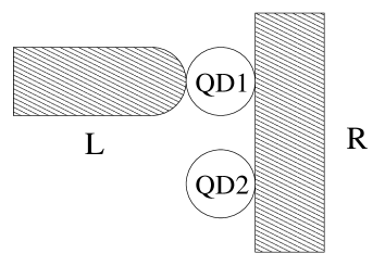
Figure 1: Schematic diagram of a system with two coupled quantum dots connected to source and drain leads in parallel. One quantum dot (QD1) is connected to both the left (L) and the right (R) external metallic leads. The other quantum dot (QD2), is only connected to R-lead.

We shall model both the L- and R-leads as one-dimensional (1D) non-interacting Fermi gases. We assume that the electron level spacing in both QDs is large in comparison with the level broadening due to the tunneling process and the thermal effect. Thus, the spectra of both QDs are discrete. For simplicity, we consider that there is only one energy level with spin degeneracy in each QD. The electron-electron (e-e) interaction in a mesoscopic system is usually larger than or comparable to other energy scales like the typical level spacing and the thermal energy. Hence the Coulomb blockade effect plays an important role in electron transport when QDs are weakly coupled to external leads. We shall consider the e-e interaction in our model. And we shall describe the tunneling process between leads and QDs with a tunneling Hamiltonian.

The total Hamiltonian of this system can be expressed as

$$H=H_{L,R}+H_{c}+H_{T},$$ (1)

where $H_{L,R}$ is the Hamiltonian of two 1D ideal metallic leads, $H_{c}$ is the Hamiltonian of the central region with two coupled QDs, and $H_{T}$ is the tunneling Hamiltonian.

The Hamiltonian of two 1D ideal metallic leads is

$$H_{L,R}=\sum_{l,k,\sigma}\epsilon_{l,k}c_{l,k\sigma}^{\dagger}c_{l,k\sigma},$$ (2)

where $\sigma=\uparrow,\downarrow$ is the spin index, and $c_{l,k\sigma}^{\dagger}$ ($c_{l,k\sigma}$) is the creation (annihilation) operator of an electron with energy $\epsilon_{l,k}$ and spin $\sigma$ in lead $l=L,R$, the left or right leads.

The Hamiltonian of the central region is

$$H_{c} =\sum_{i=1,2\atop\sigma}\epsilon_{i}d_{i\sigma}^{\dagger}d_{i\sigma}+\sum_{\sigma}\bigl{(}td_{1\sigma}^{\dagger}d_{2\sigma}+\mathrm{H.c.}\bigr{)}$$

$$\qquad\qquad+\sum_{i=1,2}U_{i}n_{i\uparrow}n_{i\downarrow},$$ (3)

where $d_{i\sigma}^{\dagger}(d_{i\sigma})$ is the creation (annihilation) operator of an electron with energy $\epsilon_{i}$ and spin $\sigma$ in QD $i$. $t$ is the hopping energy between the states $\epsilon_{1}$ and $\epsilon_{2}$ in the two QDs. The terms containing $U_{i}$ describe the e-e interactions in QD $i$.

The tunneling Hamiltonian is given as

$$H_{T}=\sum_{l,k,\sigma\atop i=1,2}V_{l,k\sigma,i}c_{l,k\sigma}^{\dagger}d_{i\sigma}+\mathrm{H.c.},$$ (4)

where $V_{l,k\sigma,i}$ is the coupling constant between state $\epsilon_{l,k}$ in the lead $l$ and state $\epsilon_{i}$ in the QD $i$. Here we assume that the tunneling process conserves electron spins.

By using the non-equilibrium Green function method, the current for a steady state is given asHaug ; Datta ,

$$I=\sum_{\sigma}\frac{e}{h}\int dE\;\mathrm{Tr}\bigl{(}\Sigma^{L,<}_{\sigma}G^{>}_{\sigma}-\Sigma^{L,>}_{\sigma}G^{<}_{\sigma}\bigr{)},$$ (5)

where $G^{<(>)}_{\sigma}$ is the lesser (greater) Green function of the central region with spin $\sigma$. $\Sigma^{L,<(>)}_{\sigma}$ is the lesser (greater) self-energy matrix of the spin $\sigma$ electron in the central region with the contribution from L-lead only. Below, we shall briefly outline the steps of calculating these Green functions. We shall see that the self-energies can be treated as parameters and their values can be chosen according to our considerations.

The lesser (greater) Green function can be calculated by the Keldysh equations,

$$G^{<(>)}_{\sigma}=G^{r}_{\sigma}\Sigma^{<(>)}_{\sigma}G^{a}_{\sigma},$$ (6)

where $G^{r(a)}_{\sigma}$ is the retarded (advanced) Green function of the central region with spin $\sigma$. $\Sigma^{<(>)}_{\sigma}$ is the lesser (greater) self-energy of spin $\sigma$ electron in the central region with the contribution from both leads.

The matrix elements of the retarded and advanced Green functions are defined as

$$G^{r}_{\sigma,ij}(t-t^{\prime}) =-i\theta(t-t^{\prime})\langle\{d_{i\sigma}(t),d_{j\sigma}^{\dagger}(t^{\prime})\}\rangle,$$ (7a)

$$G^{a}_{\sigma,ij}(t-t^{\prime}) =i\theta(t^{\prime}-t)\langle\{d_{i\sigma}(t),d_{j\sigma}^{\dagger}(t^{\prime})\}\rangle,$$ (7b)

where $\theta(t)$ is the step function, and $\{a,b\}=ab+ba$ is the Fermion anti-commutator.

The equation-of-motion method is used to calculate the retarded (advanced) Green function, $G^{r(a)}_{\sigma}$. The time derivative of the retarded (advanced) Green function $G^{r(a)}_{\sigma}$ is

$$i\frac{\partial}{\partial t}G^{r(a)}_{\sigma}=\delta(t-t^{\prime})I+AG^{r(a)}_{\sigma}+UG^{r(a)(2)}_{\sigma}+\Sigma^{r(a)}_{\sigma},$$ (8)

where

$$A=\begin{pmatrix}\epsilon_{1}&t\\ t&\epsilon_{2}\end{pmatrix},\qquad U=\begin{pmatrix}U_{1}&0\\ 0&U_{2}\end{pmatrix},$$ (9)

and $I$ is the unity matrix. $\Sigma^{r(a)}_{\sigma}$ is the retarded (advanced) self-energy with spin $\sigma$. The elements of the second order Green function $G^{r(a)(2)}_{\sigma}$ are defined as

$$G^{r(a)(2)}_{\sigma,ij}=\mp i\theta(\pm t\mp t^{\prime})\langle\{d_{i\sigma}(t)n_{i\bar{\sigma}}(t),d_{j\sigma}^{\dagger}(t^{\prime})\}\rangle,$$ (10)

where $\bar{\sigma}$ is the opposite spin to $\sigma$, and $n_{i\bar{\sigma}}=d_{i\bar{\sigma}}^{\dagger}d_{i\bar{\sigma}}$.

Usually the equation-of-motion of the Green function $G^{r(a)}_{\sigma}$ contains higher order correlation functions, for example, $G^{r(a)(2)}_{\sigma}$ in Eq. (8). When we calculate the equations-of-motion of these higher order correlation functions, even higher order correlation functions appear. In order to close those equations, we must truncated those equations at an appropriate order. Here, we only keep those equations containing terms of correlation functions up to the second order. Then, we can get the expression of $G^{r(a)}_{\sigma}$ by solving these equations. Since the calculation process is well established, we don’t give it explicitly here. The detail calculation can be found in Ref. Haug .

The retarded (advanced) Green function $G^{r(a)}_{\sigma}$ contains terms with the average electron numbers of the opposite spin, $\langle n_{i\bar{\sigma}}\rangle\;(i=1,2)$, in QD $i$. The average electron number in QD $i$ can be calculated by

$$\langle n_{i\bar{\sigma}}\rangle=\int\frac{dE}{2\pi}\;\mathrm{Im}G^{<}_{\bar{\sigma},ii}(E).$$ (11)

Thus, we need to calculate them self-consistently. After evaluating the average electron numbers in both QDs self-consistently, we can obtain all Green functions. Because we consider here a system with two QDs, all these Green functions and self-energies are $2\times 2$ matrices.

As shown above, we need to know self-energies to calculate those Green functions. The elements of lesser (greater) self-energy $\Sigma^{<(>)}_{\sigma}$ are given as

$$\Sigma^{<(>)}_{\sigma,ij} =\sum_{l,k}V_{l,k\sigma,i}V_{l,k\sigma,j}^{*}g^{l,<(>)}_{\sigma,k}$$

$$=\Sigma_{\sigma,ij}^{L,<(>)}+\Sigma_{\sigma,ij}^{R,<(>)},$$ (12)

where

$$\Sigma^{L,<(>)}_{\sigma,ij}=\sum_{k}V_{L,k\sigma,i}V_{L,k\sigma,j}^{*}g^{L,<(>)}_{\sigma,k},$$ (13a)

$$\Sigma^{R,<(>)}_{\sigma,ij}=\sum_{k}V_{R,k\sigma,i}V_{R,k\sigma,j}^{*}g^{R,<(>)}_{\sigma,k},$$ (13b)

are the lesser and greater self-energies with contributions from both L- and R-leads, respectively. $g^{l,<(>)}_{\sigma}$ is lesser (greater) Green function for lead $l$ with spin $\sigma$ and the elements of these two Green functions are given as

$$g^{l,<}_{\sigma,k}(t-t^{\prime}) =i\langle c_{l,k\sigma}^{\dagger}(t^{\prime})c_{l,k\sigma}(t)\rangle$$

$$=if_{l}(\epsilon_{l,k})e^{-i\epsilon_{l,k}(t-t^{\prime})},$$ (14a)

$$g^{l,>}_{\sigma,k}(t-t^{\prime}) =-i\langle c_{l,k\sigma}(t)c_{l,k\sigma}^{\dagger}(t^{\prime})\rangle$$

$$=-i\bigl{(}1-f_{l}(\epsilon_{l,k})\bigr{)}e^{-i\epsilon_{l,k}(t-t^{\prime})},$$ (14b)

where $f_{l}(\epsilon)=(1+e^{\beta(\epsilon-\mu_{l})})^{-1}$ is the Fermi-Dirac distribution function. $\mu_{l}$ is the chemical potential in lead $l$ and $\beta=1/(k_{B}T)$. The time dependent operators in lead $l$ are $c_{l,k\sigma}(t)=e^{-i\epsilon_{l,k}t}c_{l,k\sigma}$, $c_{l,k\sigma}^{\dagger}(t)=e^{i\epsilon_{l,k}t}c_{l,k\sigma}^{\dagger}$.

The elements of the retarded (advanced) self-energy are given as

$$\Sigma^{r(a)}_{\sigma,ij}=\sum_{l,k}V_{l,k\sigma,i}V_{l,k\sigma,j}^{*}g^{l,r(a)}_{\sigma,k},$$ (15)

where $g^{l,r(a)}_{\sigma}$ is the retarded (advanced) Green function of lead $l$ with spin $\sigma$ and their elements are given as

$$g^{l,r(a)}_{\sigma,k}(t-t^{\prime}) =\mp i\theta(\pm t\mp t^{\prime})\langle\{c_{l,k\sigma}(t),c_{l,k\sigma}^{\dagger}(t^{\prime})\}\rangle$$

$$=\mp i\theta(\pm t\mp t^{\prime})e^{-i\epsilon_{l,k}(t-t^{\prime})}.$$ (16)

In our calculation, we need to know the Fourier transformation of the elements of the retarded (advanced) self-energy. They are

$$\Sigma^{r(a)}_{\sigma,ij}(E) =\sum_{l,k}V_{l,k\sigma,i}V_{l,k\sigma,j}^{*}g^{l,r(a)}_{\sigma,k}(E)$$

$$=\Lambda^{r(a)}_{\sigma,ij}(E)\mp\frac{i}{2}\Gamma^{r(a)}_{\sigma,ij}(E).$$ (17)

where the real and imaginary parts, that is, the level-shift function $\Lambda^{r(a)}_{\sigma}(E)=\Lambda^{L,r(a)}_{\sigma}(E)+\Lambda^{R,r(a)}_{\sigma}(E)$, and the level-width function $\Gamma^{r(a)}_{\sigma}(E)=\Gamma^{L,r(a)}_{\sigma}(E)+\Gamma^{R,r(a)}_{\sigma}(E)$ are due to the tunneling process between the QDs and both L- and R-leads. Usually, these functions are energy-dependent. However, under the wide band approximation, they do not depend on electron energy. We shall use this wide band approximation and assume the level-shift and level-width functions to be independent of energy. In the absence of a magnetic field, they do not depend on spin index $\sigma$, and we shall drop it in our notations below. Therefore, we can define those self-energies as parameters with four $2\times 2$ constant matrices $\Lambda^{L(R)}$ and $\Gamma^{L(R)}$ instead of using the coupling constant $\{V_{l,k\sigma,i}\}$. Then the retarded (advanced) self-energy is

$$\Sigma^{r(a)}_{\sigma}=\Lambda^{L}+\Lambda^{R}\mp\frac{i}{2}(\Gamma^{L}+\Gamma^{R})$$ (18)

According to Eq. (II), the lesser self-energy is given as

$$\Sigma^{<}_{\sigma}(E)=i\bigl{(}\Gamma^{L}f_{L}(E)+\Gamma^{R}f_{R}(E)\bigr{)}$$ (19)

and the greater self-energy is

$$\Sigma^{>}_{\sigma}(E)=-i\bigl{(}\Gamma^{L}(1-f_{L}(E))+\Gamma^{R}(1-f_{R}(E))\bigr{)}.$$ (20)

The lesser and greater self-energies depend on energy only through the Fermi-Dirac distribution function $f_{L(R)}(E)$.

The Green functions can be calculated by equation-of-motion method described above in terms of all the self-energies. Then we can evaluate the $I$-$V$ curve by using Eq. (5). In the next section, we shall give some numerical results of $I$-$V$ curves for different cases.

III Numerical results and discussion

III.1 In the absence of e-e interactions in both QDs

First, we consider a simple case that the electron-electron (e-e) interactions in both QDs are absent, i.e., $U_{1}=U_{2}=0$. The energy needed to add an extra electron in a QD due to the e-e interaction is $e^{2}/C$, where $C$ is the capacitance of the QD. When the size of a QD are large, this energy may be very small compared to the level spacing. We can then ignore the e-e interactions in the QD. Thus, this may be used to describe a relative large QD.

In order to investigate the resonance coupling effect on the $I$-$V$ characteristics, we assume that as shown in Fig. 1 one of two QDs (QD1) is connected to both external leads while the other one (QD2) is only connected to the right lead. When no external bias is applied, electronic state energy $\epsilon_{1}(0)$ in QD1 is set to be smaller than energy $\epsilon_{2}(0)$ in QD2. The external bias is applied by increasing chemical potential $\mu_{L}$ of the left lead and keeping $\mu_{R}$ of the right lead unchanged. We assume that the barriers between QD1 and left and right leads are symmetric, and voltage drops uniformly across the QD1. Thus, the energy level $\epsilon_{1}$ of QD1 shifts to $\epsilon_{1}=\epsilon_{1}(0)+eV/2$ under a bias $V$ bias. In reality, because of the difference of the electro-static potentials of QD1 and R-lead, there is a voltage drop in QD2 and energy $\epsilon_{2}$ in QD2 should also shift. However, $\epsilon_{1}$ shifts more than $\epsilon_{2}$ does. When a certain bias is applied, $\epsilon_{1}$ and $\epsilon_{2}$ can be tuned to be aligned with each other, or resonance coupling. In fact, other model parameters may also change. It is known that bias dependence of other model parameters may also affect $I$-$V$ characteristicssdwang . However, for simplicity, we assume that the energy level $\epsilon_{2}$ in QD2 remains unchanged because we are interested in the resonance coupling effect on the $I$-$V$ curves in this study. This assumption may affect the positions of $I-V$ peaks mentioned below, it shall not change the physics studied. We shall come back to this point in our discussions.

Accordingly, we set the energies of two electronic states in the two QDs at zero bias, $\epsilon_{1}(0)=1.0$, $\epsilon_{2}(0)=3.5$. Since QD1 are connected to both leads and QD2 are only connected to the right leads, we set $\Gamma^{L}_{11}=\Gamma^{R}_{11}=0.2$, $\Gamma^{L}_{22}=0.0$, $\Gamma^{R}_{22}=0.2$, $\Gamma^{L}_{12}=\Gamma^{L}_{21}=0.0$, $\Gamma^{R}_{12}=\Gamma^{R}_{21}=0.1$. Because the level-shift functions $\Lambda^{L(R)}$ only add a constant energy shifting to the electronic state in each QD, their values don’t change our final results. We set them to zero, that is, $\Lambda^{L(R)}_{ij}=0.0$, where $i,j=1,2$. The chemical potentials of the left lead $\mu_{L}=eV$ can vary while $\mu_{R}=0$. All these parameters are in an arbitrary unit of energy $\Gamma$ which is a system parameter.

We first calculate $I$-$V$ curves at a very low temperature, $T=0.01$ in the unit of $\Gamma/k_{B}$, so that we can neglect the thermal broadening of energy levels in QDs. Fig. 2(a) shows the calculated $I$-$V$ curve and Fig. 2(b) shows the numerical result of the bias dependence of the average electron numbers $\langle n_{i}\rangle$ in QD $i$. At low and high bias, the two electronic states are far apart. Since QD2 is connected to the right lead only, electrons can only tunnel into it through QD1. In the absence of any inelastic processes, the chance for an electron tunneling from QD1 to QD2 is very small when the two electronic states, $\epsilon_{1}$ and $\epsilon_{2}$, are far apart. Therefore, the average electron number in QD2 is almost zero. Its effect on the tunneling process is negligible, and the $I$-$V$ characteristics should be very similar to that of a single QD system. This is indeed what we can see from Fig. 2(a). As shown in Fig. 2(a), there is a peak at $V=5.0$, where two electronic states $\epsilon_{1}$ and $\epsilon_{2}$ are aligned with each other. Correspondingly, the average electron number in QD1, $\langle n_{1}\rangle$ has a valley at this bias as shown in Fig. 2(b). At the same time, there is a dramatical increase in the average electron number in QD2. This is not surprising at all. The chance for an electron tunneling from one electronic state in QD1 to another state in QD2 increases as the energies of the two states approach each other. It become maximum when they are precisely aligned. We shall call it resonance coupling of the two QDs when this happens. At resonance coupling, a new tunneling channel through QD2 opens. In another words, the effective tunneling rate of an electron out of the QD dimer increases. This causes the peak observed in Fig. 2(a), leading to a NDR.

Figure 2: Numerical results of $I$-$V$ and $\langle n_{i}\rangle$-$V$ in the absence of e-e interactions. The parameters are $\epsilon_{1}(0)=1.0$, $\epsilon_{2}(0)=3.5$, $\Gamma^{L}_{11}=\Gamma^{R}_{11}=0.2$, $\Gamma^{L}_{22}=0.0$, $\Gamma^{R}_{22}=0.2$, $\Gamma^{L}_{12}=\Gamma^{L}_{21}=0.0$, $\Gamma^{R}_{12}=\Gamma^{R}_{21}=0.1$, $\Lambda^{L(R)}_{ij}=0.0$ ($i,j=1,2$), $\mu_{L}=eV$ and $\mu_{R}=0$, where all these parameters are in unit of $\Gamma$. The temperature $T=0.01$ in unit of $\Gamma/k_{B}$. (a) Current $I$ vs applied bias $V$. The current $I$ has a peak at $V=5.0$. (b) Average electron numbers in both QDs, $\langle n_{i}\rangle$ vs applied bias $V$. $\langle n_{1}\rangle$ has a valley while $\langle n_{2}\rangle$ has a peak at $V=5.0$.

This can be understood from the following argument. As the electron tunneling probability from QD1 to QD2 increases, the effective tunneling rate out of the electronic state $\epsilon_{1}$ increases and the effective tunneling rate into the electronic state $\epsilon_{2}$ increases as well. Therefore, $\langle n_{1}\rangle$ decreases and $\langle n_{2}\rangle$ increases because more electrons tunnel from QD1 to QD2. For the sequential tunneling, the resonant tunneling current and the average electron number in the resonant level at zero temperature are given asDatta

$$\langle n\rangle \propto\frac{\Gamma^{\mathrm{in}}}{\Gamma^{\mathrm{in}}+\Gamma^{\mathrm{out}}}$$ (21a)

$$I \propto\frac{\Gamma^{\mathrm{in}}\Gamma^{\mathrm{out}}}{\Gamma^{\mathrm{in}}+\Gamma^{\mathrm{out}}}$$ (21b)

where $\Gamma^{\mathrm{in}(\mathrm{out})}$ is the tunneling rate of an electron into (out of) the resonant level. Near the resonance coupling, for QD1, the tunneling rate $\Gamma^{\mathrm{in}}_{1}$ from the left lead into the dot remains almost unchanged and the tunneling rate $\Gamma^{\mathrm{out}}_{1}$ out of the dot increases because of a new tunneling channel through QD2. For QD2, the tunneling rate $\Gamma^{\mathrm{in}}_{2}$ from QD1 into QD2 increases while the tunneling rate $\Gamma^{\mathrm{out}}_{2}$ out of QD2 into the right lead remains unchanged. Therefore, the overall tunneling rates for the QD dimer is as follows. The tunneling rate $\Gamma^{\mathrm{in}}$ from left lead into the QD dimer is almost unchanged, while the effective tunneling rate $\Gamma^{\mathrm{out}}$ out of the QD dimer increases. Therefore, the total current increases and $\langle n_{1}\rangle$ decreases while $\langle n_{2}\rangle$ increases according to Eq. (21). In turn, it generates a $I$-$V$ peak and a NDR.

Figure 3: Numerical results of $I$-$V$ curves at different hopping energies and temperatures. All other parameters are the same as those in Fig. 2. (a) $I$-$V$ at different hopping energies, $t=-0.05$ (solid line), $t=-0.10$ (dashed line), and $t=-0.30$ (dotted line). The peak height and width increase as the hopping energy $t$. (b) $I$-$V$ at different temperatures, $T=0.01$ (solid line), $T=0.50$ (dashed line), and $T=1.00$ (dotted line). The peak is smeared at high temperatures.

We have seen that resonance coupling between two dots can lead to a peak in the $I$-$V$ curve. Thus, we should expect the height and width of this peak to depend on the interdot coupling strength. Also, the thermal energy can introduce inelastic tunneling processes which can wash out the resonance effect. One should also expect that the peak is also sensitive to the temperature. The $I$-$V$ curves at different interdot coupling strengths between two QDs, and at different temperatures are shown in Fig. 3(a) and (b), respectively. As shown in Fig. 3, the peak height and width increase as the coupling between two QDs increases. Because the chance of an electron tunneling from QD1 to QD2 increases with the interdot coupling, more electrons can tunnel out of the dimer through QD2, and the effective tunneling rate out of the QD dimer increases. Therefore the peak height and width increase as the interdot coupling increases. We can also see the thermal smearing of the NDR. The peak disappears gradually with the increase of temperature.

III.2 The presence of e-e interactions in QDs

In order to see whether the $I$-$V$ peaks, thus the NDR, due to the resonance coupling of two QDs will survive when the e-e interaction is present, we repeat the above calculation by including non-zero $U_{1}$ and $U_{2}$. We set the Coulomb interactions $U_{1}=U_{2}=5.0$ while keeping the other parameters the same as those in Fig. 2. The calculated results of $I$-$V$ curve and the bias dependence of the average electron numbers $\langle n_{i}\rangle$ in QD $i$ are shown in Fig. 4(a) and (b), respectively. As one will expect, the peak at $V=5.0$ is still there with the similar features as those in the absence of the e-e interaction. The reason for the occurrence of this peak should be the same as that in the previous section.

Figure 4: Numerical results of $I$-$V$ and $\langle n_{i}\rangle$-$V$ in the case in presence of e-e interactions. The e-e interactions in two QDs are $U_{1}=U_{2}=5.0$ and other parameters are the same as those in Fig. 2. (a) Current $I$ vs applied bias $V$. The current $I$ has two peaks. one is at $V=5.0$ and the other is at $V=15.0$. (b) Average electron numbers in both QDs, $\langle n_{i}\rangle$ vs applied bias $V$. $\langle n_{1}\rangle$ has a valley at $V=5.0$ and a peak at $V=15.0$. $\langle n_{2}\rangle$ has two peaks. One is at $V=5.0$ and the other is at $V=15.0$.

However, there is an extra peak at $V=15.0$. This new peak can be attributed to the e-e interactions in QDs. In order to understand the origin of this new peak, let us examine the possible electronic states in QD $i$. In the case that no electron in the QD, an electron of energy $\epsilon_{i}$ can move in freely into it. However, only the electron with energy $\epsilon_{i}+U_{i}$ can jump into the QD when there is already one electron in because of the e-e interaction. Therefore, the electronic states of the QD has effectively two distinct energy values, $\epsilon_{i}$ and $\epsilon_{i}+U_{i}$. We have already identify the first peak as the resonance coupling due to the alignment $\epsilon_{1}$ and $\epsilon_{2}$. It is natural to expect another peak to appear when $\epsilon_{1}$ is aligned with $\epsilon_{2}+U_{2}$. In our case, it corresponds to $V=15.0$, exactly what we see in Fig. 4(a). In comparison with the first peak, the second peak is smaller and narrower. This is due to the different properties of the two electronic states $\epsilon_{2}$ and $\epsilon_{2}+U_{2}$. Unlike $\epsilon_{2}$, $\epsilon_{2}+U_{2}$ doesn’t exist unless one electron has already been in QD2. However, when $\epsilon_{1}$ and $\epsilon_{2}+U_{2}$ are aligned, $\epsilon_{2}$ and $\epsilon_{1}$ are far apart. Therefore, the probability of an electron hopping from $\epsilon_{1}$ to $\epsilon_{2}$ is small. Consequently, the average electron number in $\epsilon_{2}$ is very small. Thus, the existing probability of $\epsilon_{2}+U_{2}$ state is very small too. This is probably the reason why the second peak is smaller and narrower.

Unlike the first resonance-coupling peak where $\langle n_{2}\rangle$ is maximum and $\langle n_{1}\rangle$ is minimum, both $\langle n_{1}\rangle$ and $\langle n_{2}\rangle$ are maximum at the second peak. $\langle n_{2}\rangle$ becomes maximum at the second resonance-coupling peak because the effective tunneling rate into QD2 from QD1 increases as $\epsilon_{1}$ approach $\epsilon_{2}+U_{2}$. The maximum of $\langle n_{1}\rangle$ is because both tunneling rate into and out of QD1 increase. Around $V=15.0$, the effective tunneling rate out of QD1 increases because more electrons can tunnel from QD1 to QD2. On the other hand, the effective tunneling rate into QD1 increases too. Two electrons can now be in QD1 at the same time, occupying $\epsilon_{1}$ and $\epsilon_{1}+U_{1}$ states, respectively. After the electron with energy $\epsilon_{1}$ tunnels out of QD1, the remaining electron has energy $\epsilon_{1}$ instead of its original energy $\epsilon_{1}+U_{1}$. Then a new electron with energy $\epsilon_{1}+U_{1}$ can tunnel from the left lead into QD1. As $\epsilon_{1}$ and $\epsilon_{2}+U_{2}$ are aligned, electrons in $\epsilon_{1}$ tunnel out of QD1 faster. Therefore, electrons can tunnel into QD1 from the left lead faster and the effective tunneling rate into QD1 increases. So when $\epsilon_{1}$ and $\epsilon_{2}+U_{2}$ are aligned, both the effective tunneling rate into QD1 $\Gamma^{\mathrm{in}}_{1}$ and the effective tunneling rate out of QD1 $\Gamma^{\mathrm{out}}_{1}$ increase. According to Eq. (21) the average electron number in $\epsilon_{1}$ may increase if $\Gamma^{\mathrm{in}}_{1}$ increases faster than $\Gamma^{\mathrm{out}}_{1}$. This explains the possibility that $\langle n_{1}\rangle$ reaches maximum value at the second peak.

In the above calculations, we have not considered the case that $\epsilon_{1}+U_{1}$ is aligned with $\epsilon_{2}+U_{2}$. This is because the bias is too small to allow electrons tunneling through $\epsilon_{1}+U_{1}$, when those two electronic states are aligned. Moreover, if we set the same e-e interactions in two QDs, $\epsilon_{1}+U_{1}$ and $\epsilon_{2}+U_{2}$ are aligned at the same time when $\epsilon_{1}$ and $\epsilon_{2}$ are aligned. These two effects may not be distinguished easily. In order to avoid this possible confusion, we consider different e-e interactions in two QDs such that $\epsilon_{1}$ and $\epsilon_{2}$ are not aligned with each other when $\epsilon_{1}+U_{1}$ and $\epsilon_{2}+U_{2}$ do. We also choose a set of parameters in such a way that electrons can tunnel through $\epsilon_{1}+U_{1}$ when it is aligned with $\epsilon_{2}+U_{2}$.

Figure 5: Numerical results of $I$-$V$ and $\langle n_{i}\rangle$-$V$ in the case of asymmetric e-e interactions of two QDs. The e-e interactions in two QDs are $U_{1}=3.0$ and $U_{2}=5.0$. All other parameters are the same as those in Fig. 2. (a) Current $I$ vs applied bias $V$. The current $I$ has four peaks. one is at $V=5.0$, one at $V=15.0$, and other two small peaks at $V=8.3$ and $V=8.6$, respectively. (b) Average electron numbers in both QDs, $\langle n_{i}\rangle$ vs applied bias $V$. $\langle n_{1}\rangle$ has a valley at $V=5.0$ and three peaks. The first is at $V=8.3$, the second at $V=8.6$, and the third at $V=15.0$. $\langle n_{2}\rangle$ has three peaks. One is at $V=5.0$, one at $V=8.6$, and the last at $V=15.0$.

Fig. 5(a) shows $I$-$V$ curve with $U_{1}=3.0$, $U_{2}=5.0$, and all other parameters are the same as those in Fig. 2. Besides two peaks at $V=5.0$ and $V=15.0$, there are two additional very small peaks. One is at $V=8.3$ and the other at $V=8.6$. Similar to the two old resonance-coupling peaks, these two new small peaks are due to the alignment of $\epsilon_{1}+U_{1}$ and $\epsilon_{2}+U_{2}$. This resonance-coupling yields two peaks instead of one because of the competition of two opposite effects that do not exist in the previous case. As we explain above, the existing probability of electronic state $\epsilon_{2}+U_{2}$ decrease as $\epsilon_{1}$ and $\epsilon_{2}$ are far apart. However, when $\epsilon_{1}+U_{1}$ and $\epsilon_{2}+U_{2}$ become closer, the electron tunneling probability from $\epsilon_{1}+U_{1}$ to $\epsilon_{2}+U_{2}$ increases. The competition of these two effects leads to those two peaks in the $I$-$V$ curve.

As shown in Fig 5(b), $\langle n_{1}\rangle$ has one valley at $V=5.0$ and three peaks. They are located at $V=8.3$, $8.5$, and $15.0$, respectively. $\langle n_{2}\rangle$ has three peaks at $V=5.0$, $8.5$, and $15.0$, respectively. The behavior of $\langle n_{i}\rangle$, $i=1,2$, at $V=5.0$ and $15.0$ has been already explained before. The reason of the occurrence of the other two peaks of $\langle n_{1}\rangle$ is due to the competition of two opposite effects mentioned above. When $\epsilon_{1}+U_{1}$ and $\epsilon_{2}+U_{2}$ are aligned, there are those two opposite effects. One decreases the average electron number in QD2 while the other increases it. But the increase of the average electron number is larger than the decrease of it, therefore we can only see one peak of $\langle n_{2}\rangle$.

Figure 6: Numerical results of $I$-$V$ curves at different coupling strengths and e-e interactions. All other parameters are the same as those in Fig. 2. (a) $I$-$V$ at different hopping energies, $t=-0.05$ (solid line), $t=-0.10$ (dashed line), and $t=-0.30$ (dotted line). The e-e interactions are $U_{1}=U_{2}=5.0$. (b) $I$-$V$ at different e-e interactions, $U_{1}=U2=3.0$ (solid line), $U_{1}=U_{2}=5.0$ (dashed line), and $U_{1}=U_{2}=1.00$ (dotted line).

The $I$-$V$ curves of different coupling strengths and e-e interactions are shown in Fig. 6(a) and (b), respectively. As one will expect, the heights and widths of both peaks increase as the coupling strength between two QDs increases. From Fig. 6(b), one can see that the e-e interactions have no effect on the peak at low bias because the peak at low bias is due to the alignment of $\epsilon_{1}$ and $\epsilon_{2}$. A strong e-e interaction shifts the position of the peak at high bias, but it does not change its height and width. The peak at high bias is due to the alignment of $\epsilon_{1}$ and $\epsilon_{2}+U_{2}$. As we have explained before, the height and width of this peak depend on the existing probability of $\epsilon_{2}+U_{2}$ state. When $\epsilon_{1}$ and $\epsilon_{2}+U_{2}$ are aligned, $\epsilon_{1}$ and $\epsilon_{2}$ are far apart. Thus the probability of an electron hopping from $\epsilon_{1}$ to $\epsilon_{2}$ is too small to be sensitive to the change of the e-e interactions. Consequently, the existing probability of $\epsilon_{2}+U_{2}$ state is independent of the e-e interactions. Therefore, the strong e-e interactions have little effect on the height and width of this peak. The $I$-$V$ curves at different temperatures are shown in Fig. 7. Peaks disappear at hight temperature due to the thermal smearing effects.

Figure 7: Numerical results of $I$-$V$ curves at different temperatures, $T=0.01$ (solid line), $T=0.50$ (dashed line), and $T=1.00$ (dotted line). All other parameters are the same as those in Fig. 2. Peaks are smeared at high temperatures.

Figure 8: Schematic diagrams of the wave functions of an electron in (a) off-resonance coupling and (b) resonance coupling cases. $\varphi_{1}$ and $\varphi_{2}$ are eigenfunctions with energy $\varepsilon_{1}$ and $\varepsilon_{2}$ in two QDs without interdot coupling. $\varphi$ is the wave function (bonding state) in the presence of the coupling. (a) In off-resonance coupling case, the overlap of $\varphi_{1}$ and $\varphi_{2}$ in two QDs is negligible and an electron in the bonding state is largely localized in QD1. (b) In resonance coupling case, the overlap of $\varphi_{1}$ and $\varphi_{2}$ are very large and electron in the bonding state has approximately the same probability of being found in either one of the two QDs.

What is seen is a new mechanism for the NDR in a system with more than one QDs. The NDR is a very important phenomenon and has many important applications. Devices with the NDR have been widely used to make amplifier and oscillators in a very wide frequency rangesze . In superlattice, it is known that a NDR leads to many interesting phenomena, such as current-voltage oscillation on the sequential resonant tunneling plateau, current self-oscillation, and chaosxrw . There are many mechanisms for NDR, such as Gunn effect and resonant tunneling in superlattices. The NDR found here is due to the resonance coupling between two QDs. As shown in Fig. 8, the wave function of the bonding state is largely localized in QD1 in off-resonance case. Electrons can only tunnel from the source to the drain through QD1. In resonance coupling case, electrons in the bonding state can be in both QDs, and electrons can also tunnel from the source to the drain through QD2. A new tunneling channel is open and a peak can be observed in the $I$-$V$ curve. This leads to the NDR. Furthermore, the properties of the NDR depend on the properties of both QDs. For example, the widths and heights of peaks vary as the dot-dot coupling. And the positions of peaks depend on the energy spectra of both QDs. The variations of the energy spectra of the QD under the probing tip or the adjacent QD, or both QDs may change the positions of peaks in $I$-$V$ curves. Thus, the $I$-$V$ characteristics shall have different behavior when the tip is above QD2 rather than QD1. Comparing this difference will allow one to distinguish a NDR due to the mechanism proposed here from the others. A better understanding of this resonance coupling effect may also enhance the STM as a powerful probe not only for a regular surface, but also for a cluster structure.

We show that an $I$-$V$ peak, thus NDR, appears at the resonance coupling between two QDs where their energy levels are aligned. For simplicity, we consider essentially only one electronic state in each QD. The mechanism should survive in the case that there are more than one electronic state in each QD. This effect should be pronounced when the sizes of QDs are small such that the discrete natural of electronic state are clear. We assume also that the bias shifts only the energy levels in the QD directly connected to two leads and has no effect on other parameters. In reality, the bias not only shifts the energy levels of both QDs but also changes the tunneling ratessdwang . But in our quantum dot configuration, which may arise in a STM experiments, the energy levels in QD1 shall be affected more than those in QD2 by an external bias. Thus, the resonance coupling will occur under certain bias. We use this simplified assumption in order to unambiguously identify the observed $I$-$V$ peaks. Since the physics is due to the resonance coupling which indeed should occur in real experiments, we believe this new mechanism is very robust, and does not depend on our assumption. Of course, the peak positions, which are not our main concern, depend surely on the assumption. In fact, the NDR due to the resonance coupling of two QDs may have been observed already in a recent experimentgwang .

IV Summary

In summary, the dot-dot coupling effect on the tunneling current under a bias is investigated. We considered a QD dimer connected to two metallic leads in such a way that one QD in the dimer is connected to the both leads while the other is only directly connected to one lead. We show numerically that peaks, thus NDRs, appear in the $I$-$V$ curves at resonance coupling when two electronic states in two QDs are aligned. This NDR exists both in the absence and in the presence of e-e interactions. We study how the peaks in the $I$-$V$ characteristics change with interdot coupling, e-e interaction, and the temperature. We show that the heights and widths of those peaks increase with the interdot coupling of the QD dimer. But they are almost unaffected by the e-e interactions in both QDs when the e-e interactions are strong. We show that those peaks are smeared at high temperatures due to the thermal smearing effects.

- (1) M. A. Kastner, Phys. Today 46, 24 (1993).
- (2) T. J. Thornton, Rep. Prog. Phys. 58, 311 (1995); C. G. Smith, Rep. Prog. Phys. 59, 235 (1996).
- (3) C. H. Bennett, Phys. Today 48, 24 (1995); D. P. DiVincenzo, Science 270, 255 (1995); A. Barenco et al., Phys. Rev. Lett. 74, 4083 (1995); A. Steane, Rep. Prog. Phys. 61, 117 (1998); D. Loss and D. P. DiVincenzo, Phys. Rev. A 57, 120 (1998); P. Zanardi and F. Rossi, Phys. Rev. Lett. 81, 4752 (1998).
- (4) L. P. Kouwenhoven et al., Phys. Rev. Lett. 65, 361 (1990); F. R. Waugh et al., Phys. Rev. Lett. 75, 705 (1995).
- (5) N. C. van der Vaart et al., Phys. Rev. Lett. 74, 4702 (1995).
- (6) L. Kouwenhoven, Science 268, 1440 (1995); G. Schedelbeck et al., Science 278, 1792 (1997); R. H. Blick et al., Phys. Rev. Lett. 80, 4032 (1998) A. W. Holleitner et al., Science 297, 70 (2002).
- (7) I. M. Ruzin et al., Phys. Rev. B 45, 13469 (1992); G. W. Bryant, Phys. Rev. B 48, 8024 (1993); C. A. Stafford and S. Das Sarma, Phys. Rev. Lett. 72, 3590 (1994); G. Klimeck et al., Phys. Rev. B 50, 2316 (1994); K. A. Matveev et al., Phys. Rev. B 53, 1034 (1996); J. M. Golden and B. I. Halperin, Phys. Rev. B 53, 3893 (1996).
- (8) C. Y. Fong et al., Phys. Rev. B 46, 9538 (1992).
- (9) J. J. Palacios and P. Hawrylak, Phys. Rev. B 51, 1769 (1995).
- (10) H. Haug and A.-P. Jauho, Quantum Kinetics in Transport and Optics of Semiconductors (Springer, 1996); G. D. Mahan, Many-particle physics, 2nd ed. (New York, Plenum Press, c1990).
- (11) S. Datta, Computer Electronic transport in mesoscopic systems (Cambridge University Press, Cambridge, 1995);
- (12) S. D. Wang, Z. Z. Sun, N. Cue, H. Q. Xu, and X. R. Wang, Phys. Rev. B 65, 125307 (2002).
- (13) S. M. Sze, Modern semiconductor device physics (J. Wiley, New York 1998).
- (14) X. R. Wang and Q. Niu, Phys. Rev. B. 59, R12755 (1999); J. N. Wang, B. Q. Sun, X. R. Wang, W. Ge, and H. Wang, Appl. Phys. Lett. 75, 2620 (1999); X. R. Wang, J. N. Wang, B. Q. Sun, and D. S. Jiang, Phys. Rev. B 61, 7261 (2000).
- (15) G. Wang, in Similarities and differences between atomic nuclei and clusters, eds. Y. Abe et al., Tsukuba, Japan, AIP Conference Proceedings 416, 338 (1997).