Classical technical analysis of Latin American market indices. Correlations in Latin American currencies ($ARS$, $CLP$, $MXP$) exchange rates with respect to $DEM$, $GBP$, $JPY$ and $USD$

Abstract

The classical technical analysis methods of financial time series based on the moving average and momentum is recalled. Illustrations use the IBM share price and Latin American (Argentinian MerVal, Brazilian Bovespa and Mexican IPC) market indices. We have also searched for scaling ranges and exponents in exchange rates between Latin American currencies ($ARS$, $CLP$, $MXP$) and other major currencies $DEM$, $GBP$, $JPY$, $USD$, and $SDR$s. We have sorted out correlations and anticorrelations of such exchange rates with respect to $DEM$, $GBP$, $JPY$ and $USD$. They indicate a very complex or speculative behavior.

Keywords: Econophysics; Detrended Fluctuation Analysis; Foreign Currency Exchange Rate; Special Drawing Rights; Scaling Hypothesis; Technical Analysis; Moving Average; Argentinian MerVal, Brazilian Bovespa and Mexican IPC

1 Introduction

The buoyancy of the US dollar is a reproach to stagnant Japan, recessing Europe economy and troubled developing countries like Brazil or Argentina. Econophysics aims at introducing statistical physics techniques and physics models in order to improve the understanding of financial and economic matters. Thus when this understanding is established, econophysics might $later$ help in the well being of humanity. In so doing several techniques have been developed to analyze the correlations of the fluctuations of stocks or currency exchange rates. It is of interest to examine cases pertaining to rich or developing economies.

In the first sections of this report we recall the classical technical analysis methods of stock evolution. We recall the notion of moving averages and (classical) momentum. The case of IBM and Latin American market indices serve as illustrations.

In 1969 the International Monetary Fund created the special drawing rights $SDR$, an artificial currency defined as a basket of national currencies $DEM$, $FRF$, $USD$, $GBP$ and $JPY$. The $SDR$ is used as an international reserve asset, to supplement members existing reserve assets (official holdings of gold, foreign exchange, and reserve positions in the IMF). The $SDR$ is the IMF’s unit of account. Four countries maintain a currency peg against the $SDR$. Some private financial instruments are also denominated in $SDR$s.[1, 2] Because of the close connections between the developing countries and the IMF, we search for correlations between the fluctuations of $ARS$, $CLP$ and $MXP$ exchange rates with respect to $SDR$ and the currencies that form this artificial money. In the latest sections of this report, we compare the correlations of such fluctuations as we did in our previous results on $EUR$ exchange rates fluctuations with respect to $USD$, $GBP$ and $JPY$ [3, 4, 5].

2 Technical Analysis: IBM and Latin America Markets

Technical indicators as moving average and $momentum$ are part of the classical technical analysis and much used in efforts to predict market movements [6]. One question is whether these techniques provide adequate ways to read the trends.

Consider a time series $x(t)$ given at N discrete times $t$. The series (or signal) moving average $M_{\tau}(t)$ over a time interval $\tau$ is defined as

$$M_{\tau}(t)=\frac{1}{\tau}\sum_{i=t}^{t+\tau-1}x(i-\tau)\qquad t=\tau+1,\dots,N$$ (1)

i.e. the average of $x$ over the last $\tau$ data points. One can easily show that if the signal $x(t)$ increases (decreases) with time, $M_{\tau}(t)<x(t)$ ($M_{\tau}(t)>x(t)$). Thus, the moving average captures the trend of the signal given the period of time $\tau$. The IBM daily closing value price signal between Jan 01, 1990 and Dec 31, 2000 is shown in Fig. 1 (top figure) together with Yahoo moving average taken for $\tau=50$ days [7]. The bottom figure shows the daily $volume$ in millions.

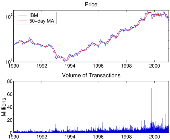
Figure 1: IBM daily closing value signal between Jan 01, 1990 and Dec 31, 2000, i.e. 2780 data points with Yahoo moving average for $\Delta T$ = 50 day. (top); the bottom figure shows the daily volume

There can be as many trends as moving averages as $\tau$ intervals. The shorter the $\tau$ interval the more sensitive the moving average. However, a too short moving average may give false messages about the long time trend of the signal. In Fig. 2(a) two moving averages of the IBM signal for $\tau$=5 days (i.e. 1 week) and 21 days (i.e. 1 month) are compared for illustration.

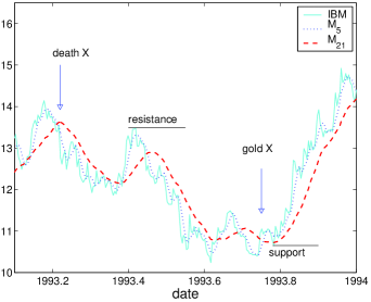
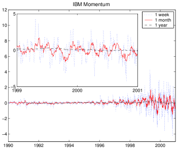
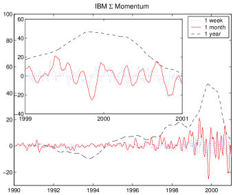
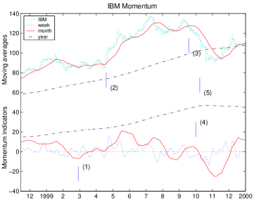
Figure 2: (a) IBM daily closing value signal between Jan 01, 1990 and Dec 31, 2000, with two moving averages, $M_{\tau_{1}}$ and $M_{\tau_{2}}$ for $\tau_{1}=5$ days and $\tau_{2}=21$ days. (b) IBM classical momentum (c) moving average of IBM classical momentum for three different time periods $\tau$, 1 week (dot curve), 1 month (solid curve) and 1 year (dot-dash curve). (d) IBM signal and the six market indicators for three time horizons, short-term (weekly) (dot curve), medium-term (monthly) (solid curve) and log-term (yearly) (dot-dash curve). IBM original signal and its moving averages are divided by 10 for readability

The intersections of the price signal with a moving average can define so-called lines of resistance or support [6]. A line of resistance is observed when the local maximum of the price signal $x(t)$ crosses a moving average $M_{\tau}(t)$. A support line is defined if the local minimum of $x(t)$ crosses $M_{\tau}(t)$. In Fig. 2(a) lines of resistance happen around May 1993 and lines of support around Sept 1993. Support levels indicate the price where the majority of investors believe that prices will move higher, and resistance levels indicate the price at which a majority of investors feel prices will move lower. Other features of the trends are the intersections between $two$ moving averages $M_{\tau_{1}}$ and $M_{\tau_{2}}$ which are usually due to drastic changes in the trend of $x(t)$ [8]. Consider two moving averages of IBM price signal for $\tau_{1}=5$ days and $\tau_{2}=21$ days (Fig. 2(a)). If $x(t)$ increases for a long period of time before decreasing rapidly, $M_{\tau_{1}}$ will cross $M_{\tau_{2}}$ from above. This event is called a ”death cross” in empirical finance [6]. In contrast, when $M_{\tau_{1}}$ crosses $M_{\tau_{2}}$ from below, the crossing point coincide with an upsurge of the signal $x(t)$. This event is called a ”gold cross”. Therefore, it is of interest to study the density of crossing points between two moving averages as a function of the size difference of the $\tau$’s defining the moving averages. Based on this idea, a new and efficient approach has been suggested in Ref.[8] in order to estimate an exponent that characterizes the roughness of a signal.

The so called $momentum$ is another instrument of the technical analysis and we will refer to it here as the classical momentum, in contrast to the generalized momentum [9]. The classical momentum of a stock is defined over a time interval $\tau$ as

$$R_{\tau}(t)=\frac{x(t)-x(t-\tau)}{\tau}=\frac{\Delta x}{\Delta t}\qquad t=\tau+1,\dots,N$$ (2)

The momentum $R_{\tau}$ for three time intervals, $\tau=5,21$ and 250 days, i.e. one week, one month and one year, are shown in Fig. 2(b) for IBM. The longer the period the smoother the momentum signal. Much information on the price trend turns is usually considered to be found in a moving average of the momentum

$$R^{\Sigma}_{\tau}(t)=\sum_{i=t}^{t+\tau-1}\frac{x(i)-x(i-\tau)}{\tau}\qquad t=\tau+1,\dots,N$$ (3)

Moving averages of the classical momentum over 1 week, 1 month and 1 year for the IBM price difference over the same time intervals, $R^{\Sigma}_{\tau}$ are shown in Fig. 2(c). In Fig. 2(d) the IBM signal and its weekly (short-term), monthly (medium-term) and yearly (long-term) moving averages are compared to the weekly (short-term), monthly (medium-term) and yearly (long-term) momentum indicators in order to better observe the bullish and bearish trends in 1999.

The message that is coming out of reading the combination of the these six indicators states that one could start buying at the momentum bottom, as it is for both monthly and weekly momentum indicators around mid February 1999 and buy the rest of the position when the price confirms the momentum uptrend and rises above the monthly moving average which is around March 1999. The first selling signal is given during the second half of July 1999 by the death cross between short and medium term moving averages and by the maximum of the monthly momentum, which indicates the start of a selling. At the beginning of October 1999, occurs the maximum of the long-term momentum. It is recommended that one can sell the rest of the position since the price is falling down below the moving average. Hence, it is said that momentum indicators lead the price trend. They give signals before the price trend turns over.

Along the lines of the above for IBM, we analyze three Latin America financial indices, Argentinian MerVal, Brazilian Bovespa and Mexican IPC (Indice de Precios y Cotizaciones) applying the moving averages and the classical momentum concepts. In Fig. 3 the time evolution of the MerVal stock over the time interval mid 1996 - mid 2001, is plotted with a simple moving average for $\tau=$50 days showing the medium range trend of the price. The moving average and classical momentum of the MerVal stock prices for time horizons equal to one week, one month and one year are shown Fig. 3.

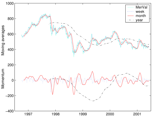
Figure 3: Argentinian MerVal daily closing value signal between Oct 08, 1996 and Jun 06, 2001, i.e. 1162 data points; classical momentum for three time horizons, short-term (weekly) (dot curve), medium-term (monthly) (solid curve) and log-term (yearly) (dot-dash curve)

The cases of the Brazilian Bovespa and Mexican IPC (Indice de Precios y Cotizaciones) are shown in Figs. 4 and 5 respectively.

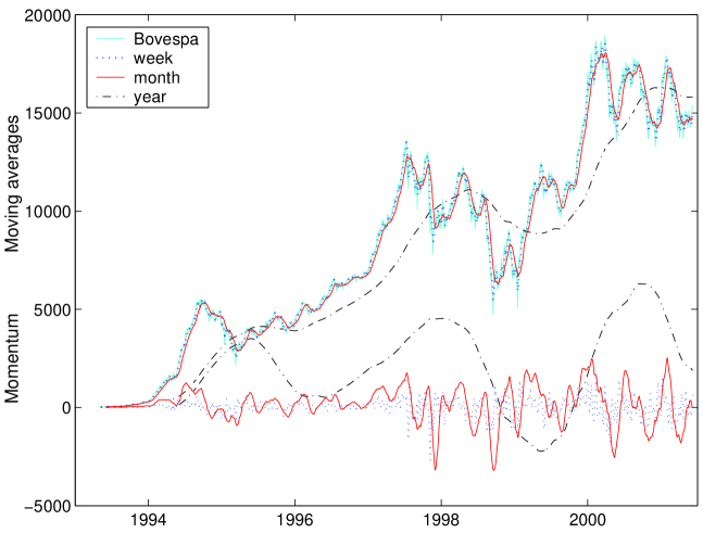
Figure 4: Brazilian Bovespa daily closing value signal between April 27, 1993 and Jun 06, 2001, i.e. 2010 data points; classical momentum for three time horizons, short-term (weekly) (dot curve), medium-term (monthly) (solid curve) and log-term (yearly) (dot-dash curve)

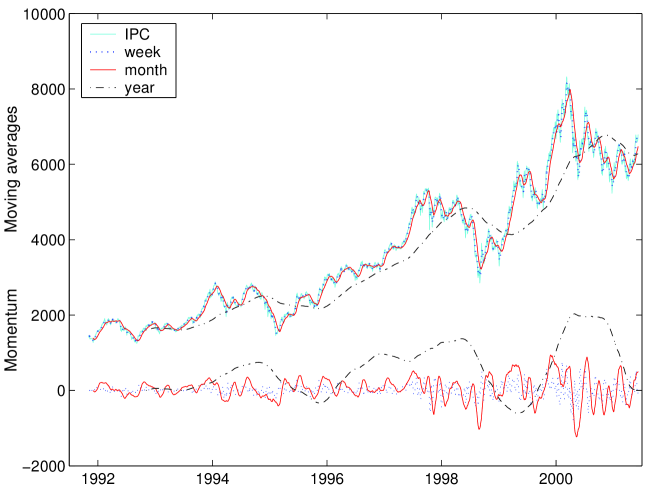
Figure 5: Mexican IPC daily closing value signal between Nov. 08, 1991 and Jun 06, 2001, i.e. 2384 data points; classical momentum for three time horizons, short-term (weekly) (dot curve), medium-term (monthly) (solid curve) and log-term (yearly) (dot-dash curve)

3 Exchange Rates and Special Drawing Rights

In 1969 the International Monetary Fund (IMF) created the Special Drawing Rights (ticker symbol $SDR$; sometimes $XDR$ is also used), an artificial currency unit defined a basket of national currencies. The $SDR$ is used as an international reserve asset, to supplement members’ existing reserve assets (official holdings of gold, foreign exchange, and reserve positions in the IMF). The $SDR$ is the IMF’s unit of account: IMF voting shares and loans are all denominated in $SDR$s. The $SDR$ serves as the unit of account for a number of other international organizations, including the WB. Four countries maintain a currency peg against the $SDR$. Some private financial instruments are also denominated in $SDR$s.

The basket is reviewed every five years to ensure that the currencies included in the basket are representative of those used in international transactions and that the weights assigned to the currencies reflect their relative importance in the world’s trading and financial systems. Following the completion of the most recent regular review of $SDR$ valuation on October 11, 2000, the IMF’s Executive Board agreed on changes in the method of valuation of the $SDR$ and the determination of the $SDR$ interest rate, effective Jan. 01, 2001.

The $SDR$ artificial currency can be represented as an weighted sum of the five currencies $C_{i}$, $i=1,5$:

$$1SDR=\sum_{i=1}^{5}\gamma_{i}\,C_{i}$$ (4)

where $\gamma_{i}$ are the currencies weights in percentage (Table 1) and $C_{i}$ denote the respective currencies, U.S. Dollar ($USD$), German Mark ($DEM$), French Franc ($FRF$), Japanese Yen ($JPY$), British Pound ($GBP$).

Table 1: Currency Weights in $SDR$ Basket (In Percent)

Currency	Last Revision	Revision of
	January 1, 2001	January 1, 1996
$USD$	45	39
$EUR$	29
$DEM$		21
$FRF$		11
$JPY$	15	18
$GBP$	11	11

On January 1, 1999, the German Mark and French Franc in the $SDR$ basket were replaced by equivalent amounts of $EUR$. The relevant exchange rates (ExR) are shown in Figs. 6-8.

Figure 6: Exchange rates of $ARS$ with respect to $SDR$, $USD$, $DEM$, $JPY$, $GBP$ for the time interval between Aug. 6, 1996 and May 31, 2001, i.e. 1208 data points, as available on http://pacific.commerce.ubc.ca/xr/ website

Figure 7: Exchange rates of $CLP$ with respect to $SDR$, $USD$, $DEM$, $JPY$, $GBP$ for the time interval between Nov. 16, 1995 and May 31, 2001, i.e. 1376 data points, as available on http://pacific.commerce.ubc.ca/xr/ website

Figure 8: Exchange rates of $MXP$ with respect to $SDR$, $USD$, $DEM$, $JPY$, $GBP$ for the time interval between July 7, 1993 and May 31, 2001, i.e. 1975 data points, as available on http://pacific.commerce.ubc.ca/xr/ website

3.1 The DFA technique

The DFA technique [10] is often used to study the correlations in the fluctuations of stochastic time series like the currency exchange rates. Recall briefly that the DFA technique consists in dividing a time series $y(t)$ of length $N$ into $N/\tau$ nonoverlapping boxes (called also windows), each containing $\tau$ points [10]. The local trend $z(n)$ in each box is defined to be the ordinate of a linear least-square fit of the data points in that box. The detrended fluctuation function $F^{2}(\tau)$ is then calculated following:

$$F^{2}(\tau)={1\over\tau}{\sum_{n=k\tau+1}^{(k+1)\tau}{\left[y(n)-z(n)\right]}^{2}}\qquad k=0,1,2,\dots,\left(\frac{N}{\tau}-1\right)$$ (5)

Averaging $F^{2}(\tau)$ over the $N/\tau$ intervals gives the mean-square fluctuations

$$\phi(\tau)=<F^{2}(\tau)>^{1/2}\sim\tau^{\alpha}$$ (6)

The exponent $\alpha$ value implies the existence or not of long-range correlations, and is assumed to be identical to the Hurst exponent when the data is stationary. Moreover, $\alpha$ is an accurate measure of the most characteristic (maximum) dimension of a multifractal process [11]. Since only the slopes and scaling ranges are of interest the various DFA-functions $\phi(\tau)$ have been arbitrarily displaced for readability in Figs. 9-11. The $\alpha$ values are summarized in Table 2. It can be noted that the scaling ranges are usually from 5 days till 170 days for $ARS$ exchange rates, from 5 days to about 1 year for $MXP$ and $CLP$ exchange rates, with the exponent $\alpha$ close to 0.5 in that range. Crossover at  80 days from Brownian like to persistent correlations is obtained for $CLP/JPY$ and $CLP/SDR$.

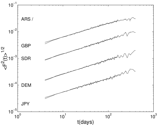
Figure 9: DFA-function $\phi(\tau)$ function for the $ARS$ Exchange rates shown in Fig. 6; the various $\phi(\tau)$ have been arbitrarily displaced for readability

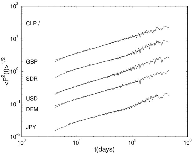
Figure 10: DFA-function $\phi(\tau)$ function for the $CLP$ Exchange rates shown in Fig. 7; the various $\phi(\tau)$ have been arbitrarily displaced for readability

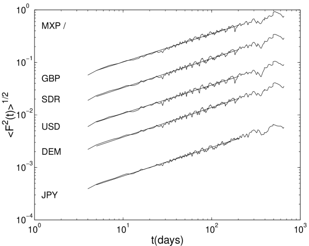
Figure 11: DFA-function $\phi(\tau)$ function for the $MXP$ Exchange rates shown in Fig. 8; the various $\phi(\tau)$ have been arbitrarily displaced for readability

Table 2: $\alpha$ exponent for the scaling regime of considered ExR in the text

	$USD$	$DEM$	$GBP$	$JPY$	$SDR$
$ARS/$		0.54$\pm$0.02	0.51$\pm$0.02	0.51$\pm$0.02	0.54$\pm$0.02
$CLP/$	0.54$\pm$0.03	0.50$\pm$0.02	0.51$\pm$0.03	0.46$\pm$0.02	0.45$\pm$0. 01
				0.70$\pm$0.07	0.74$\pm$0.07
$MXP/$	0.54$\pm$0.03	0.56$\pm$0.03	0.54$\pm$0.03	0.55$\pm$0.02	0.56$\pm$0. 03

3.2 Local scaling with DFA and Intercorrelations between fluctuations

The time derivative of $\alpha$ can usually be correlated to an entropy production [12] through market information exchanges. As done elsewhere, in order to probe the existence of locally correlated and decorrelated sequences, we have constructed an observation box, i.e. a 500 days wide window probe placed at the beginning of the data, calculated $\alpha$ for the data in that box. Moving this box by one day toward the right along the signal sequence and again calculating $\alpha$, a local $\alpha$ exponent is found (but not displayed here).

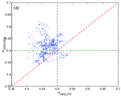
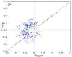
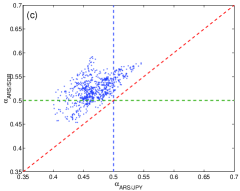
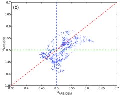
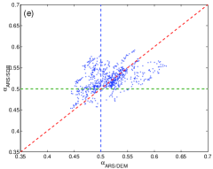
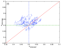
Figure 12: Structural correlation diagram of (a-f) between typical $\alpha_{C_{i}/B_{j}}$ exponents for exchange rates between $ARS$ and $DEM$, $GBP$, $JPY$, $SDR$

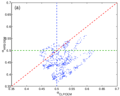
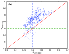
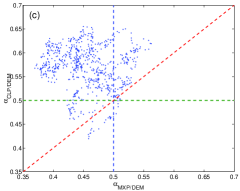
Figure 13: Structural correlation diagram of (a-c) between typical $\alpha_{C_{i}/B_{j}}$ exponents for exchange rates, i.e. involving $ARS$, $MXP$, $CLP$ and $DEM$

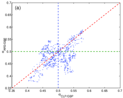
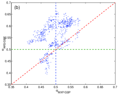
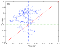
Figure 14: Structural correlation diagram of (a-c) between typical $\alpha_{C_{i}/B_{j}}$ exponents for exchange rates, i.e. involving $ARS$, $MXP$, $CLP$ and $GBP$

We eliminate the time between these data sets and construct a graphical correlation matrix of the time-dependent $\alpha$ exponents for the various exchange rates of interest (Fig.12-14). We show $\alpha_{C_{i}/B_{j}}$ vs. another $\alpha_{C_{i}/B_{j}}$, where a $C_{i}$ is a developing country currency while $B_{j}$ is $USD$, $GBP$, $JPY$, $DEM$, and $SDR$ for the available data. In so doing a so-called correlation matrix is displayed for the time interval of interest. Such bilateral correlations between different $\alpha$ exponents can be considered in order to estimate the strength and some nature of the correlations. As described elsewhere [4], such a correlation diagram can be divided into main sectors through a horizontal, a vertical and diagonal lines crossing at (0.5,0.5). If the correlation is strong the cloud of points should fall along the slope $=+1$ line. If there is no correlation the cloud should be rather symmetrical. The lack of symmetry of the plots and wide spreading of points outside expected clouds (see e.g. Figs. 13(c), 14(b,c) - mainly containing $MXP$) indicate highly speculative situations. Notice the marked imbalance of some plots, mainly involving $ARS$. It is fair to say that other techniques are also of great interest to observe correlations between financial markets [13, 14, 15].

4 Conclusions

The classical technical analysis methods of financial indices, stocks, futures, … are very puzzling. We have recalled them. Illustrations have used the IBM share price and Latin American financial indices. We have used the DFA method to search for scaling ranges and type of behavior of exchange rates between Latin American currencies ($ARS$, $CLP$, $MXP$) and other major currencies $DEM$, $GBP$, $JPY$ and $USD$, including $SDR$s. In all cases persistent to Brownian like behavior is obtained for scaling ranges from a week to about one year, with an exception of $CLP/JPY$ and $CLP/SDR$ for which there is a transition from Brownian like to persistent correlations with $\alpha=0.70$ and $\alpha=0.74$ for scaling ranges longer than 80 days. We have also sorted out to correlations and anticorrelations of such exchange rates with respect to currencies as $DEM$, $GBP$, $JPY$ and $USD$. They indicate a very complex or speculative behavior.

Acknowledgements

MA thanks to the organizers of the Stauffer 60th birthday symposium for their invitation and kind welcome.

References

- [1] http://www.imf.org/external/np/tre/sdr/basket.htm
- [2] http://www.imf.org/external/np/tre/sdr/drates/0701.htm
- [3] M. Ausloos and K. Ivanova, Physica A 286, 353 (2000).
- [4] K. Ivanova and M. Ausloos, Eur. Phys. J. B 20, 537 (2001).
- [5] K. Ivanova and M. Ausloos, in Empirical sciences in financial fluctuations. The advent of econophysics H. Takayasu, Ed. (Springer Verlag, Berlin, 2002) pp. 62-76
- [6] see S.B. Achelis, in http://www.equis.com/free/taaz/
- [7] http://finance.yahoo.com
- [8] N. Vandewalle and M. Ausloos, Phys. Rev. E, 58, 6832 (1998).
- [9] M. Ausloos and K. Ivanova, Eur. Phys. J. B 27, 177 (2002).
- [10] C.-K. Peng, S.V. Buldyrev, S. Havlin, M. Simmons, H.E. Stanley and A.L. Goldberger, Phys. Rev. E 49, 1685 (1994).
- [11] K. Ivanova and M. Ausloos, Eur. Phys. J. B 8, 665 (1999).
- [12] N. Vandewalle and M. Ausloos, Physica A 246, 454 (1997).
- [13] H. Fanchiotti, C.A. García Canal, H. García Zúñiga, Int. J. Mod. Phys. C 12, 1485 (2001).
- [14] R. Mansilla, Physica A 301, 483 (2001).
- [15] S. Maslov, S. Maslov, Physica A 301, 397 (2001).