Singlet-triplet transition in a lateral quantum dot

Abstract

We study transport through a lateral quantum dot in the vicinity of the singlet-triplet transition in its ground state. This transition, being sharp in an isolated dot, is broadened to a crossover by the exchange interaction of the dot electrons with the conduction electrons in the leads. For a generic set of system’s parameters, the linear conductance has a maximum in the crossover region. At zero temperature and magnetic field, the maximum is the strongest. It becomes less pronounced at finite Zeeman splitting, which leads to an increase of the background conductance and a decrease of the conductance in the maximum.

The Kondo effect in transport through quantum dots manifests itself in a dramatic increase of the linear conductance at temperatures below a certain characteristic scale $T_{K}$ (the Kondo temperature). In the simplest case kondo , a quantum dot behaves essentially as a magnetic impurity with spin 1/2 coupled via exchange interaction to two conducting leads GP_review . However, the energy scale for intradot excitations is much smaller than the corresponding scale for real magnetic impurities. Moreover, the tunability of this scale in quantum dot devices allows one to explore various flavors of the Kondo effect inaccessible with usual magnetic impurities induced_review .

A transition between singlet and triplet states in an almost isolated dot was demonstrated Tarucha in a “vertical” device. At stronger dot-lead tunneling, the conductance across the dot has a pronounced maximum at the singlet-triplet transition Sasaki . The maximum can be interpreted induced_review ; EN ; ST as the Kondo effect with the Kondo temperature enhanced in the vicinity of the transition. In this paper, we investigate the conductance in a “lateral” quantum dot device in the vicinity of a singlet-triplet transition. The presented below theory of the Kondo effect in such devices may help in the interpretation of the recent experiments vanderWiel ; Kogan .

The main difference between vertical dots and lateral ones is that in the latter case the number of electronic modes coupled to a quantum dot is well defined. A lateral quantum dot is formed by gate depletion of a two-dimensional electron gas at the interface between two semiconductors. In this geometry the dot-leads junctions act as electronic waveguides. Potentials on the gates control the waveguide width, and, therefore, the number of propagating electronic modes the waveguides support: by making the waveguide narrower one pinches the propagating modes off. When the very last propagating mode nears its pinch-off, the system enters the Coulomb blockade regime. Accordingly, in this regime each dot-lead junction supports a single electronic mode MF .

Typically, the charging energy of the dot $E_{C}$ is large compared to the mean single-particle level spacing in it, $\delta E$, which in turn guarantees GP_review that $\delta E$ is large compared to $T_{K}$: $T_{K}\ll\delta E\ll E_{C}$. This separation of the energy scales allows us to simplify the problem further by assuming that conductances of the dot-lead junctions are small. The simplification will not affect the properties of the system in the Kondo regime as long as $T_{K}$ remains the smallest energy scale in the problem. On the other hand, the coupling between the dot and the leads can now be described within the tunneling Hamiltonian framework. The microscopic Hamiltonian of the system can then be written as a sum of three distinct terms,

$$H=H_{\rm leads}+H_{\rm dot}+H_{\rm tunneling},$$ (1)

which describe, respectively, free electrons in the leads, isolated quantum dot, and the tunneling between the dot and the leads. With only one electronic mode for each dot-lead junction taken into account, the first and the third terms in the r.h.s. of Eq. (1) become

$$H_{\rm leads} = \sum_{\alpha ks}\xi^{\phantom{\dagger}}_{k}c^{\dagger}_{\alpha ks}c^{\phantom{\dagger}}_{\alpha ks},\quad\alpha=R,L$$ (2)

$$H_{\rm tunneling} = \sum_{\alpha nks}t^{\phantom{\dagger}}_{\alpha n}c^{\dagger}_{\alpha ks}d^{\phantom{\dagger}}_{ns}+{\rm H.c.}$$ (3)

A generic model of an isolated quantum dot [the second term in the r.h.s. of Eq. (1)] can be written as ABG

$$H_{\rm dot}=\sum_{ns}\epsilon_{n}^{\phantom{\dagger}}d^{\dagger}_{ns}d^{\phantom{\dagger}}_{ns}+E_{C}\left(\hat{N}-\mathcal{N}\right)^{2}-E_{S}\hat{\bm{S}}^{2}-B\hat{S}^{z},$$ (4)

where $\hat{N}=\sum_{ns}d^{\dagger}_{ns}d^{\phantom{\dagger}}_{ns}$ and $\hat{\bm{S}}=\frac{1}{2}\sum_{nss^{\prime}}d^{\dagger}_{ns}\hat{\bm{\sigma}}_{ss^{\prime}}d^{\phantom{\dagger}}_{ns^{\prime}}$ are operators of the total number of electrons on the dot, and of the dot’s spin, respectively. The parameter $\mathcal{N}$ in Eq. (4) is proportional to the potential on the capacitively coupled gate electrode and controls the number of electrons, $N=\langle\hat{N}\rangle$, on the dot. We will assume that $\mathcal{N}$ is tuned to a Coulomb blockade valley with an even number of electrons $N$. The third term in Eq. (4) describes exchange interaction within the dot. Finally, the last term in Eq. (4) represents the Zeeman effect of an external magnetic field, with $B$ being the Zeeman energy.

We consider a dot in a state far from the ferromagnetic instability ABG : the exchange energy $E_{S}$ is small compared to the mean level spacing $\delta E$. Under this condition the ground state of an isolated dot with even $N$ is almost always a singlet. The only exception occurs when the level spacing $\varepsilon=\epsilon_{+1}-\epsilon_{-1}$ between the highest occupied ($n=-1$) and the lowest empty ($n=+1$) single-particle energy levels is anomalously small, $\varepsilon\sim E_{S}\ll\delta E$. The gain in the exchange energy associated with a formation of the triplet state may then be sufficient to overcome the loss in the kinetic energy (cf. the Hund’s rule in atomic physics). The triplet state is formed through a redistribution of two electrons between the levels $n=\pm 1$. Since for an isolated dot the occupation $\sum_{s}d^{\dagger}_{ns}d^{\phantom{\dagger}}_{ns}$ on each single-particle energy level is a constant of motion, the redistribution must involve tunneling between the levels $n=\pm 1$ and the leads. At low energies ($B,T\ll\delta E$) tunneling to all other ($n\neq\pm 1$) energy levels can be neglected in the vicinity of the singlet-triplet transition ($\varepsilon\sim E_{S}$). Accordingly, in this regime the Hamiltonian of the dot Eq. (4) can then be further truncated to that of a two-level system with $\mathcal{N}=2$ and

$$\epsilon_{n}=n\varepsilon/2,\quad n=\pm 1.$$ (5)

In quantum dot systems based on GaAs the value of $\varepsilon$ can be controlled by a magnetic field $H_{\perp}$ applied perpendicular to the plane of the dot Sasaki ; vanderWiel . Because of the smallness of the electron effective mass, even a weak field $H_{\perp}$ has a very strong orbital effect. At the same time, smallness of g-factor in GaAs ensures that the corresponding Zeeman splitting remains small induced_review . By linearizing $\varepsilon(H_{\perp})$ in the vicinity of the transition, one can make a direct comparison of the experimental data with the (calculated) linear conductance across the system $G=(2e^{2}/h)g(\varepsilon)$. In addition, one can apply a strong in-plane field $H_{\parallel}$, which would allow the study of the conductance dependence on Zeeman energy $B$. The temperature ($T$) and field ($B$) dependences of the linear conductance, and the bias dependence of the differential conductance are qualitatively similar to each other. However, the dependence $g(\varepsilon,B)$ at $T=0$ is easier to calculate, and it is this function we address here.

Tunneling, see Eq. (3), couples the two-level system, Eqs. (4) and (5), to the two leads. The four tunneling amplitudes $t_{\alpha,\pm 1}$ form a $2\times 2$ matrix

$$\hat{t}=\left(\begin{array}[]{cc}t_{L,+1}&t_{R,+1}\\ t_{L,-1}&t_{R,-1}\end{array}\right).$$

In the special case when one of the eigenvalues of $\hat{t}$ is zero, while another one is finite HS , the dot effectively interacts only with a single species (a single “channel”) of conduction electrons. A single channel can screen only half of the dot’s spin when it is in the triplet state NB . Accordingly, the system should exhibit a quantum phase transition VBH : the ground state changes its symmetry from a singlet to a doublet as $\varepsilon$ decreases below a certain value, $\varepsilon_{C}\sim E_{S}$. The conductance is then strongly $\varepsilon$-dependent HS : $g(\varepsilon,0)\propto\theta(\varepsilon_{C}-\varepsilon)$. At $\varepsilon<\varepsilon_{C}$ (when the dot is in the triplet state) the conductance is a monotonically decreasing function of $B$, while at $\varepsilon>\varepsilon_{C}$ the conductance first increases, and then drops with the increase of $B$ HS .

In the general situation, however, both eigenvalues of $\hat{t}$ are finite. Therefore, the dot is coupled to two electronic channels, which is sufficient to fully screen the it’s spin NB . As the result, the ground state of the system is a singlet at all $\varepsilon$ ST ; Izumida2 ; real . In other words, when the dot is coupled to the leads, the singlet-triplet transition turns to a crossover. In order to study this crossover, we focus on a special subset Izumida2 ; Izumida1 of the matrices $\hat{t}$ parametrized as

$$\hat{t}=\frac{1}{\sqrt{2}}\left(\begin{array}[]{cc}v_{+1}&v_{+1}\\ v_{-1}&-v_{-1}\end{array}\right).$$ (6)

Obviously, for $v_{\pm 1}\neq 0$ both eigenvalues of $\hat{t}$ are finite, so the choice Eq. (6) captures the essential physics of the system.

Since the ground state of the system is not degenerate, electrons scatter elastically at $T=0$. The amplitudes of scattering $\mathbb{S}_{s;\alpha\alpha^{\prime}}$ of an electron with spin $s$ from lead $\alpha^{\prime}$ to lead $\alpha$ form the scattering matrix $\hat{\mathbb{S}}_{s}$. The $2\times 2$ unitary matrix $\hat{\mathbb{S}}_{s}$ can be diagonalized by a rotation in the $R-L$ space to the new basis of channels $n=\pm 1$,

$$U\hat{\mathbb{S}}_{s}U^{\dagger}={\rm diag}\left\{e^{2i\delta_{ns}}\right\},\quad U=e^{i\vartheta_{0}\tau^{y}}e^{i\varphi_{0}\tau^{z}}.$$ (7)

Here $\tau^{i}$ are the Pauli matrices acting in the $R-L$ space ($\tau_{+}=\tau_{x}+i\tau_{y}$ transforms $L$ to $R$). In general, the angles $\vartheta_{0}$ and $\varphi_{0}$ in Eq. (7) depend on the parameters of the microscopic Hamiltonian, and, in particular, on the values of $\varepsilon$ and $B$. Here comes the key advantage of Eq. (6): with this choice of the tunneling amplitudes, the angles are parameter-independent constants: $\vartheta_{0}=\pi/4$, $\varphi_{0}=0$. Indeed, when written in terms of the operators

$$\psi_{nks}=\frac{1}{\sqrt{2}}\left(nc_{Rks}+c_{Lks}\right),\quad n=\pm 1,$$

[corresponding to $\vartheta_{0}=\pi/4$ and $\varphi_{0}=0$ in Eq. (7)], the Hamiltonian (1)-(6) assumes the form

$$H=\sum_{nks}\xi^{\phantom{\dagger}}_{k}\psi^{\dagger}_{nks}\psi^{\phantom{\dagger}}_{nks}+H_{\rm dot}+\sum_{nks}v^{\phantom{\dagger}}_{n}\left(\!\psi^{\dagger}_{nks}d^{\phantom{\dagger}}_{ns}+{\rm H.c.}\!\right)$$ (8)

with $H_{\rm dot}$ given by Eqs. (4), (5). For each $n$ and $s$ this Hamiltonian commutes with the operator

$$\hat{\mathbb{N}}_{ns}=\sum_{k}\psi^{\dagger}_{nks}\psi^{\phantom{\dagger}}_{nks}+d^{\dagger}_{ns}d^{\phantom{\dagger}}_{ns}$$

of the total number of electrons with spin $s$ on the “orbital” $n$. Since $\hat{\mathbb{N}}_{ns}$ commute with each other, the (non-degenerate) ground state of $H$ is also an eigenstate of $\hat{\mathbb{N}}_{ns}$. This implies that single-particle correlation functions are diagonal in $n$ and $s$, e.g., $\langle\psi^{\phantom{\dagger}}_{nks}(t)\psi^{\dagger}_{n^{\prime}k^{\prime}s^{\prime}}(0)\rangle\propto\delta_{nn^{\prime}}\delta_{ss^{\prime}}$. Therefore the scattering matrix, which can be expressed via retarded single-particle correlation functions, is diagonal in $n$ and $s$ as well.

The dimensionless conductance $g$ at $T=0$ is related to the off-diagonal elements of the scattering matrix by the Landauer formula $g=\frac{1}{2}\sum_{s}\left|\mathbb{S}_{s;RL}^{2}\right|$. With the help of Eq. (7) the conductance can be expressed via the scattering phase shifts $\delta_{ns}$ at the Fermi energy:

$$g=\frac{1}{2}\sum_{s}\sin^{2}\Delta_{s},\quad\Delta_{s}=\delta_{+1,s}-\delta_{-1,s}.$$ (9)

(here we took into account that $\vartheta_{0}=0$). The scattering phase shifts $\delta_{ns}$ in Eqs. (7) and (9) are obviously defined mod $\pi$ (that is, $\delta_{ns}$ and $\delta_{ns}+\pi$ are equivalent). This ambuguity can be removed by setting the values of the phase shifts corresponding to $\mathcal{N}=-\infty$ (when the dot is empty) to $0$. With this convention, the phase shifts at a finite $\mathcal{N}$ are expressed via the Friedel sum rule in terms of the ground state occupation numbers $N_{ns}=\langle d^{\dagger}_{ns}d^{\phantom{\dagger}}_{ns}\rangle$,

$$\delta_{ns}=\pi N_{ns}.$$ (10)

Equation (10) is exact in the limit of infinite bandwidth. Alternatively, the phase shifts can be extracted directly from the finite-size spectra obtained by the numerical renormalization group HZ .

In the Coulomb blockade valley the number of electrons on the dot is fixed: $N=\sum_{ns}N_{ns}=2$. Accordingly, the phase shifts satisfy

$$\sum_{ns}\delta_{ns}=2\pi.$$ (11)

Additional relation for the phase shifts follows from the invariance of the Hamiltonian (1)-(4) with respect to the transformation $(s,B)\to(-s,-B)$:

$$\delta_{ns}(B)=\delta_{n,-s}(-B).$$ (12)

Consider first the limit of zero field, $B=0$. From Eqs. (11) and (12) it follows that

$$\delta_{ns}(0)=\delta_{n,-s}(0)=\delta_{n},\quad\sum_{n}\delta_{n}=\pi.$$ (13)

At the triplet side of the crossover $\varepsilon\ll E_{S}$ both levels in the dot are singly occupied, so that Eq. (10) yields $\delta_{n}=\pi/2$. On the contrary, at $\varepsilon\gg E_{S}$ the level $n=-1$ is doubly occupied, while the level $n=+1$ is empty, which corresponds to $\delta_{-1}=\pi$, $\delta_{+1}=0$. When $\varepsilon$ is tuned through the crossover, the difference of the phase shifts, $\Delta_{s}=\delta_{+1}-\delta_{-1}$ [see Eq. (9)], monotonically decreases from $0$ to $-\pi$. It follows then from Eq. (9) that the dependence of the dimensionless zero-field conductance $g(\varepsilon,0)$ on $\varepsilon$ is nonmonotonic. The conductance reaches its maximum $g=1$ at some $\varepsilon=\varepsilon_{0}$ corresponding to $\Delta_{s}(\varepsilon_{0})=-\pi/2$, and falls off monotonically with the distance $|\varepsilon-\varepsilon_{0}|$ to this point, see Fig. 1. The energy $\varepsilon_{0}\simeq 2E_{S}$ may be identified with the center of the crossover region. The conductance $g\sim 1$ within this region. Later on we will relate the width of the crossover region $T_{0}$ to the parameters of the Hamiltonian (4),(8).

The effect of the Zeeman energy $B$ on the conductance accross the dot depends on how far its parameters are from the crossover point. In order to study the influence of a small $B$, one can expand the phase shifts in a series Nozieres . Taking into account Eqs. (11), (12), and (13), we obtain

$$\delta_{ns}(\varepsilon,B)=\delta_{n}+s\left({B}/{T_{n}}\right)+n\left({B}/{T^{\prime}}\right)^{2}+O(B^{3}),$$ (14)

where $n=\pm 1$, $s=\pm 1$, and $\delta_{n}$, $T_{n}$, and $T^{\prime}$ depend on $\varepsilon$. The sign of the linear in $B$ term in Eq. (14) is fixed by the following argument. The spin polarization $N_{n,+1}-N_{n,-1}$ of electrons on each level ($n=\pm 1$) grows proportionally to $B$. It follows then from Eqs. (10) and (14) that $T_{n}>0$ for $n=\pm 1$. In the next order in $B$, magnetic field favors a triplet over the singlet state of the dot. Therefore, the difference $N_{+1,s}-N_{-1,s}$ increases with $|B|$, which fixes the sign of the second order in $B$ contribution in Eq. (14).

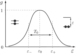
Figure 1: Dimensionless conductance across the dot at $T=0$ and $B=0$. The conductance decreases with $B$ at $\varepsilon_{-}<\varepsilon<\varepsilon_{+}$ and increases with $B$ outside this interval.

Substitution of Eq. (14) into Eq. (9) yields the low-$B$ asymptotics of the conductance,

$$g(\varepsilon,B)=g+(1-2g)\left(B/B_{0}\right)^{2}+4\sqrt{g(1-g)}\left(B/T^{\prime}\right)^{2},$$ (15)

with $g=g(\varepsilon,0)$ and

$$\frac{1}{\,B_{0}(\varepsilon)}=\left|\sum_{n=\pm 1}\frac{n}{T_{n}(\varepsilon)}\right|\,.$$ (16)

Around the crossover point $g\approx 1$, the last term in Eq. (15) vanishes, and

$$g(\varepsilon,B)\approx 1-\left(B/B_{0}\right)^{2},\quad|\varepsilon-\varepsilon_{0}|\ll T_{0}.$$ (17)

Away from the crossover ($g\ll 1$), Eq. (15) yields

$$g(\varepsilon,B)\approx g(\varepsilon,0)+\left(B/B_{0}\right)^{2},\quad|\varepsilon-\varepsilon_{0}|\gg T_{0}\,.$$ (18)

It is clear from Eqs. (17) and (18) that the conductance varies with the magnetic field in the opposite directions in the vicinity and far away from the crossover point. It should be emphasized that this is a generic property rather than a consequence of the specific choice of the model, Eq. (6). However, the precise borders of the crossover region $\varepsilon=\varepsilon_{\pm}$, see Fig. 1, as well as zero-field conductances $g(\varepsilon_{\pm},0)$ at these points are model dependent. Note also that Eq. (15) is applicable only at $B\ll B_{0}(\varepsilon)$. The conductance at higher fields is a nonmonotonic function of $B$, see Refs. real ; Izumida1 ; HZ ; Zeeman .

The Hamiltonian Eq. (8) is identical to that employed previously ST to study transport through a vertical dot. Accordingly, the thermodynamic properties of a lateral dot coincide with those of a vertical dot. However, the existing experiments test transport properties rather than thermodynamics. The electron current operators are different for the two models, hence the dependences $g(\varepsilon,B)$ are different as well. For instance, the conductance through a vertical dot at $T=0$ is large ($\sim 4e^{2}/h$) at the triplet side of the crossover and decreases with $B$, in contrast with Eq. (18).

At $|\varepsilon-\varepsilon_{0}|\gg T_{0}$ the parameters $g(\varepsilon,0)$ and $B_{0}(\varepsilon)$ entering Eq. (18) can be estimated with the help of the perturbative renormalization group ST . In this regime the $\varepsilon$-dependence of all observable quantities is governed by the parameter

$$x(\varepsilon)=(\varepsilon-\varepsilon_{0})/T_{0},\quad 1\ll\,|x(\varepsilon)|\ll\delta E/T_{0}.$$ (19)

The estimated width of the crossover region satisfies ST

$$\ln(\delta E/T_{0})\approx{\frac{E_{C}C(\gamma)}{\nu(v_{+1}^{2}+v_{-1}^{2})}},\quad\gamma=|v_{+1}/v_{-1}|,$$ (20)

where $\nu$ is density of states in the leads. The function $C(\gamma)$ has a minimum $C\approx 0.36$ at $\gamma=1$ and goes over to $1$ as $\gamma\to 0,\infty$. The scale $T_{0}$ also plays the part of the Kondo temperature as it determines the $T$-dependence of the conductance in the crossover region: the peak in $g(\varepsilon)$ disappears at $T\gg T_{0}$. Typically, $T_{0}$ is larger than the Kondo temperatures in the nearby Coulomb blockade valleys with odd number of electrons on the dot EN ; ST .

The zero-$B$ conductance entering Eq. (15) away from the crossover point (at $|x|\gg 1$) is

$$g(\varepsilon,0)\propto(\ln|x|)^{-2}.$$ (21)

Finally, the characteristic magnetic field $B_{0}(\varepsilon)$ defined in Eq. (16) has different asymptotes at the triplet and singlet sides of the crossover:

$${B_{0}}/{T_{0}}\propto\left\{\begin{array}[]{lr}|x|^{-\lambda}(\ln|x|)^{2\lambda/(\lambda+1)},&x<0,\\ \\ x(\ln x)^{2(\lambda+2)/(\lambda+1)},&x>0\end{array}\right.$$ (25)

with $\lambda=2+\sqrt{5}\approx 4.2$ and $|x|\gg 1$.

The dependence of the differential conductance $dI/dV$ on the source-drain bias $V$ at $eV\gg T,B$ is qualitatively similar to the dependence of the linear conductance on $B$ at $B\gg T$. The similarity stems from the fact that $dI/dV$ is determined by the electron transmission coefficient at energies $\omega\sim eV$, where $\omega$ is measured from the Fermi level GP_review . The dependences of the transmission coefficient on $\omega$ and $B$ are controlled by a single energy scale; the $\omega=0$ limit of the transmission coefficient governs GP_review ; real the linear conductance $g(\varepsilon,B)$. Therefore, Eq. (17) implies also that $dI/dV$ decreases with $V$ in the crossover region shown in Fig. 1. On the contrary, away from the crossover the conductance is small, $dI/dV\sim(2e^{2}/h)g(\varepsilon,0)$, in the domain $V\ll\Delta V\sim B_{0}/e$ and is increasing with $V$, cf. Eq. (18). The “window” $\Delta V$ is narrow at the triplet side of the crossover but broadens approximately linearly with the distance to the crossover at the singlet side of it, see Eq. (25). This is in agreement with numerical simulations HZ .

The zero-bias suppression of $dI/dV$ was observed in recent experiments vanderWiel ; Kogan . A measurement in the limit of very weak tunneling, necessary for the proper characterization of the spin state of the dot, was not possible for the studied devices. However, the observed vanderWiel asymmetric behavior of $\Delta V$ across the point where the conductance has a maximum is precisely the expected behavior in the vicinity of the singlet-triplet crossover. The asymmetric behavior of $\Delta V$ across the crossover may explain the observed Kogan splitting of the Kondo peak in a certain range of gate voltages.

We benefited from discussions and correspondence with S. De Franceschi, M.A. Kastner, A. Kogan, L.P. Kouwenhoven, H. Schoeller, W.G. van der Wiel, and G. Zarand. Two of us (M.P. and L.I.G.) are grateful to the Kavli Institute for Theoretical Physics at USCB and to the Institute for Nuclear Theory at the University of Washington for their hospitality. This work was supported by NSF grants DMR97-31756, DMR02-37296, and EIA02-10736. W.H. acknowledges financial support from the German Science Foundation (DFG), and L.I.G thanks the Institute for Strongly Correlated and Complex Systems at BNL for hospitality and support.

References

- (1) D. Goldhaber-Gordon et al., Nature (London) 391, 156 (1998); S.M. Cronenwett, T.H. Oosterkamp, and L.P. Kouwenhoven, Science 281, 540 (1998); J. Schmid et al., Physica (Amsterdam) 256B-258B, 182 (1998).
- (2) L.I. Glazman and M. Pustilnik, cond-mat/0302159.
- (3) M. Pustilnik et al., Lecture Notes in Physics, 579, 3 (2001).
- (4) S. Tarucha et al., Phys. Rev. Lett. 84, 2485 (2000); L.P. Kouwenhoven, D.G. Austing, S. Tarucha, Rep. Prog. Phys. 64, 701 (2001).
- (5) S. Sasaki et al., Nature 405, 764 (2000).
- (6) M. Eto and Yu.V. Nazarov, Phys. Rev. Lett. 85, 1306 (2000); Phys. Rev. B 66, 153319 (2002).
- (7) M. Pustilnik and L.I. Glazman, Phys. Rev. Lett. 85, 2993 (2000); Phys. Rev. B 64, 045328 (2001).
- (8) W.G. van der Wiel et al., Phys. Rev. Lett. 88, 126803 (2002).
- (9) A. Kogan et al., Phys. Rev. B 67, 113309 (2003).
- (10) K.A. Matveev, Phys. Rev. B 51, 1743 (1995); K. Flensberg, Phys. Rev. B 48, 11156 (1993).
- (11) I.L. Aleiner, P.W. Brouwer, and L.I. Glazman, Physics Reports 358, 309 (2002).
- (12) W. Hofstetter and H. Schoeller, Phys. Rev. Lett. 88, 016803 (2002).
- (13) P. Nozières and A. Blandin, J. Phys. (Paris) 41, 193 (1980).
- (14) M. Vojta, R. Bulla, and W. Hofstetter, Phys. Rev. B 65, 140405 (2002).
- (15) W. Izumida, O. Sakai, and S. Tarucha, Phys. Rev. Lett. 87, 216803 (2001).
- (16) M. Pustilnik and L.I. Glazman, Phys. Rev. Lett. 87, 216601 (2001).
- (17) W. Izumida, O. Sakai, and Y. Shimizu, J. Phys. Soc. Jpn. 67, 2444 (1998).
- (18) W. Hofstetter and G. Zarand, cond-mat/0306418.
- (19) P. Nozières, J. Low Temp. Phys. 17, 31 (1974); J. Phys. (Paris) 39, 1117 (1978).
- (20) M. Pustilnik, Y. Avishai, and K. Kikoin, Phys. Rev. Lett. 84, 1756 (2000).