Multilevel Monte Carlo method for simulations of fluids

Abstract

Monte Carlo methods play important part in modern statistical physics. The application of these methods suffer from two main difficulties.The first is caused by the relatively small number of particles that can participate in any numerical calculation. This means that scales larger than or comparable to the one that can be simulated are not taken into account. The second difficulty is the locality of the conventional Monte Carlo algorithms which leads to very ( sometimes unreasonably) long equilibration times. These obstacles can be eliminated in the framework of the multilevel Monte Carlo method described here. The basic approach is to describe the system at increasingly coarser levels defined on increasingly large domains, and transfer information back and forth between the levels in order to obtain a selfconsistent result. The method is illustrated for a test case of one-dimensional fluids

1 INTRODUCTION

The modern theory of classical liquids is based on the statement that the macroscopic characteristics of a many-particle system can be obtained by averaging over microscopic configurations, with the probability proportional to the Gibbs distribution function. Every microscopic configuration is defined by assigning specific locations to the particles, and the main computational problem of statistical physics consists in the difficulty of averaging over the enormous space of possible configurations. In order to estimate the value of this average the Monte Carlo technique for the canonical ensemble was proposed [1].

However, the straightforward application of this technique is restricted to a small volume of the system under consideration, because one can consider only a relatively small number of particles in any numerical calculation. In order to minimize the surface effect on the bulk values which are to be calculated, artificial periodic boundary conditions are supposed [1] similar to the case of an infinite crystal [2].

This means that at scales comparable with the periodicity cell size the fluctuations of the particle number are cut off. In order to avoid this difficulty several approaches have been suggested using the grand canonical ensemble [3],[4],[5]. The main trait of these algorithms is the generation of density fluctuations in the basic cell by adding and deleting particles in accordance with the value of the chemical potential.

The Monte Carlo simulations both in canonical and grand canonical ensembles are very local, moving, e.g., one particle at a time. The operation of adding/deleting a particle is also local and needs to be followed by a local equilibration. This leads to very slow changes of large-scale features, such as averages and various types of clusters (regions of (anti)aligned dipoles, crystallized segments, etc.).The larger the scale the slower the change and longer (per particle!) is the Monte Carlo process required to produce new independent features. Since many independent features are needed for calculating accurate averages, and since very-large-scale features need to be sampled, especially in the vicinity of phase transitions, the computations often become extremely expensive, sometimes even losing practical ergodicity. In recent years, a number of novel Monte Carlo algorithms ensuring ergodicity were proposed [6], [7], [8]. In order to avoid the slowness of the ordinary Monte Carlo simulation, steps of more collective nature are used. Nevertheless, the simulation is performed in the periodicity cell and the estimation of bulk values may only be done by extrapolation [14].

An approach which allows to simultaneously overcome slowness and finite size effects of the conventional Monte Carlo method consists of a multilevel view of the system, realized by multilevel algorithms [9], [10]. The multilevel algorithms construct a sequence of descriptions of the system under consideration at increasingly coarser levels and transfer information back and forth between the levels in order to obtain a selfconsistent result. The efficiency of multilevel methods in solving problems of statistical physics has been shown on examples with sufficiently simple systems [11]. It follows from these results that the effect of slowing down can be eliminated. Moreover, due to the possibility to simulate large volumes at coarse levels, the volume factor (the proportionality of the computational cost to the volume being simulated) can be suppressed as well. This means that the scale of treating a system is not restricted by the size of the basic cell. The elimination of both the slowing down and the volume factor allows one to investigate in the framework of the multilevel method long range phenomena such as phase transition. This possibility has been shown on two-dimensional examples of variable-coefficient Gaussian models [11] and the Ising model [13].

The successful application of the multilevel methods to lattice systems excites interest in adapting them to more complicated cases. The present paper treats multilevel algorithms to the investigation of fluids. Numerical results of simulations for one dimensional models are presented. These models reproduce common properties of fluids and allow comparisons to exact solutions.

2 MULTILEVEL MONTE CARLO APPROACH

2.1 Conventional Monte Carlo Method

The Monte Carlo method in the statistical theory of liquids is used to evaluate numerically the average $\overline{A}$ of any functional $A$, defined by:

$$\overline{A}=\int\limits_{\Omega}A(\underline{X})\cdot w(\underline{X})\cdot d\underline{X}\approx\frac{1}{m}\sum\limits^{m}_{i=1}A(\underline{X_{i}})$$ (1)

where $w(\underline{X})$ is the probability density of the state $\underline{X}$ in the configuration space $\Omega$, and the nodes $\underline{X_{i}}$ are generated by a random walk in $\Omega$ that satisfies detailed balance.

The simplest definition of the probability to walk from $\underline{X}$ to $\underline{X^{\prime}}$ in detailed balance is given by :

$$\omega(\underline{X}\to\underline{X^{\prime}})=\min\left[1,\frac{w(\underline{X^{\prime}})}{w(\underline{X})}\right]\hskip 5.69054pt,$$ (2)

provided that the probability $P(\underline{X^{\prime}}\hskip 1.42262pt?|\hskip 1.42262pt\underline{X})$ for having chosen the state $\underline{X^{\prime}}$ as the candidate to replace the current state $X$ is symmetric, i.e., $P(\underline{X^{\prime}}\hskip 1.42262pt?|\hskip 1.42262pt\underline{X})=P(\underline{X}\hskip 1.42262pt?|\hskip 1.42262pt\underline{X^{\prime}})$.

The kind of probability density given by Gibbs in the canonical ensemble for simple liquids is:

$$w(\underline{X})=\it{const}\cdot\exp(-\frac{U(\vec{r}_{1},\vec{r}_{2},\ldots,\vec{r}_{N})}{k_{B}\cdot T})$$ (3)

where $\vec{r}_{i}$ is the location of the $i$-th particle ($i=1,\ldots,N$), $k_{B}$ is the Boltzmann constant, T is the temperature and $U$ is the potential energy. It is usually assumed to have the form:

$$U=\sum\limits_{i<j}\phi(\mid\vec{r}_{i}-\vec{r}_{j}\mid)$$ (4)

where $\phi(\mid\vec{r}_{i}-\vec{r}_{j}\mid)$ corresponds to the energy of a two-body interaction.

In any numerical calculation it is possible to consider only relatively small number of particles (extremely small in comparison with Avogadro number). In order to minimize the surface effect in a small simulation volume, periodic boundary conditions are supposed [1]. This means that the space is filled by particles which are located at points:

$$\vec{R}_{i,\vec{l}}=\vec{r}_{i}+\vec{l}\cdot L,\hbox{ $1\leq i\leq N$}$$ (5)

where $\vec{l}$ is a vector whose components are integer, particles at points $\vec{r}_{i}$ are located inside the basic cell of the linear size $L$, and $N$ is the particle number in the periodicity cell.

It follows from the periodicity condition that the real system is replaced by a super-lattice with the same value of the particle number density $\rho=N/L^{D}$ (where $D$ being the dimension of the space) in each cell.

The motion of particles is continuous and in any configuration the particles have arbitrary locations. The transition between states is made by the shift of one particle at a time [1] by a small amount via the following displacement:

$$\vec{r}_{i}^{\hskip 4.2679ptnew}=\vec{r}_{i}^{\hskip 4.2679ptold}+\delta_{max}\cdot(\vec{1}-2\cdot\vec{\xi})$$ (6)

where $\vec{r}_{i}^{\hskip 4.2679ptold}$ and $\vec{r}_{i}^{\hskip 4.2679ptnew}$ are old and new locations of the $i$-th particle, $\delta_{max}$ is the maximum possible displacement of the particle along a coordinate axes, $\vec{1}$ is the vector all of whose components are $1$, and $\vec{\xi}$ is a vector whose components are random numbers distributed uniformly on the interval $[0,1]$.

For shifting the particle with the number $i$, say, one can see from (2) that it is enough to use, instead of the Gibbs function (3) with the energy (4), the conditional probability defined by:

$$P(\vec{r}_{i}\mid{\bf R_{i}})=\it{const}\cdot\exp(-u_{i}({\bf R_{i}})/k_{B}T)$$ (7)

The last relation gives us the probability to find the particle with the number $i$ at the position $\vec{r}_{i}$ when the locations of all other particles, defined by the set ${\bf R_{i}}=\{\vec{r}_{1},\ldots,\vec{r}_{i-1},\vec{r}_{i+1},\ldots,\vec{r}_{N}\}$, are fixed. The one-particle energy $u_{i}({\bf R_{i}})$ in (7) is defined by:

$$u_{i}({\bf R_{i}})=\sum\limits_{j,(j\neq i)}\phi(\mid\vec{r}_{i}-\vec{r}_{j}\mid)$$ (8)

It follows from (6) that the conventional Monte Carlo simulation is the local process. Therefore one can expect the high speed convergence only in the case of systems with short-range correlations.

2.2 Coarse variables

A slowing-down is inherent not only in the conventional Monte Carlo algorithm, it is a common problem for all local processes (e.g. Gauss- Seidel relaxation for discretizied partial differential equations). The solution to this problem lies in introducing system changes of more collective nature. In the case of partial differential equations fast convergence of solutions had been attained by multigrid algorithms [12]. These algorithms are looking for solutions on a sequence of lattices with increasingly larger meshsize (coarser scales) by combining local processing at each scale with various inter-scale (inter-lattice) interactions. A similar technique can be applied to the simulation of liquids.

A possible way to introduce a coarse description of liquid consists in the discretization of space. The periodicity cell is divided into $M$ disjoint parts (e.g. cubes) $V_{i}^{1}$ of equal volume with linear size $h_{1}$, $1\leq i\leq M$ (each $V_{i}^{1}$ being associated with a gridpoint $i$ of the first coarse-level lattice). Configurations of the finest (particle) level are mapped to the first coarse level by the operation of coarsening, this operation creates the coarse-level variable set. For example, at any instant the corresponding coarse-level variable can be defined by coarsening the particle number:

$$n_{i}^{1}=\hbox{ Number of particles in }V_{i}^{1}$$ (9)

with $\sum\limits_{i=1}^{M}n_{i}=N$, where $N$ is the total number of particles in the periodicity cell. The set $\{n_{i}^{1}\}$ defines the current configuration on the first coarse-level: instead of particle locations the occupation numbers at gridpoints are used.

Generally, the aim of coarsening is the creation of configurations represented by collective variables which describe collective particle motions at different scales. The variable at each lattice point at each coarse level is defined as a local spatial average (an average or actually a sum over a certain neighborhood of the lattice point) of similar variables at the next finer level. The total value of each such variable is well defined for each configuration of particles given at the finest level.

The extension of the coarsening operation (9) to coarser levels leads to the following definition of the coarse-variable at the level $k$:

$$n_{j}^{k}=\sum\limits_{V_{i}^{k-1}\subset V_{j}^{k}}n_{i}^{k-1},\hbox{ $k>1$}$$ (10)

for each volume element $V_{j}^{k}$ of level $k$, assuming it to be a union of volume elements of the level $k-1$. The coarsening can be repeated till the coarsest level, whose choice depends on the scale of the phenomena one wants to compute.

The coarser level simulations are performed in periodicity cells of larger sizes. In this way finite size effects are suppressed and it is possible to reach the macroscopic description of the system. No slowdown should occur provided that the coarsening ratio (the ratio between a coarse meshsize and the next finer meshsize), as well as the average number of of original particles per mesh volume of the finest lattice, are suitably low. The typical meshsize ratio is 2, typical number of particles per finest lattice mesh is between 2 and 10 (being usually larger at a higher dimension). More aggressive coarsening ratios would require much longer simulations to produce information for coarser levels.

There are many possible ways to choose the set of coarse variables. A general criterion for the quality of this set is the speed of equilibration of a compatible Monte Carlo (CMC). By this we mean a Monte Carlo process on the fine level which is restricted to the subset of fine-level configurations whose local spatial averages coincide with a fixed coarse-level configuration. A fast CMC equilibration implies that up to local processing all equilibrium configurations are fully determined by their coarse-level representations (their local spatial averages), which is the main desired property of coarsening.

The compatible Monte Carlo equilibration speed can be tested at the fine level, in the following way: after local thermalization of the ordinary Monte Carlo process, for a given configuration in the equilibrium the corresponding coarse variables are calculated by (9) or (10). Then an initial configuration in the original variables is created in accordance with the coarse variables set. A following ensemble of compatible Monte Carlo processes yields an accurate estimate of the rate of approach to the equilibrium. The interpolation from the first coarse level configuration to the finest (particle) level needs a special consideration owing to the mapping of variables defined on a grid into the continuous space of particle coordinates.

2.3 CP Tables and Multilevel Algorithm

The main idea of the multilevel approach is to equilibrate on each level only modes with short (comparable with the meshsize) wave lengths. Long wave modes with slow convergence at a given level are equilibrated at coarser levels where their wave lengths are comparable with the meshsize. As a result, the multilevel process leads to fast equilibration of all modes.

In the framework of this multilevel Monte Carlo algorithm, only a local process is performed at each level, defined in terms of the corresponding variables. In order to calculate transition probabilities (2) conditional probabilities similar to (7) should be derived for each coarse level. Such conditional probabilities are expressed in the form of a Conditional Probability (CP) table, which in principle tabulates numerically the probability distribution of any pair of neighboring coarse-level variables given the values of all others. Of course, not all other variables should in practice be taken into account: only the immediate neighborhood of gridpoint pair under test counts, due to the near locality property of the conditional probability (cf. also discussion of near locality in [13]).

For example, in terms of variables (9), (10) defined at gridpoints a conditional probability tables $P_{k}(n^{k}_{i},n^{k}_{j}\mid s^{1}_{i},\ldots,s^{l}_{i})$ can be constructed from a given sequence of configurations in equilibrium on the next finer level $k-1$. These tables give us the dependence of the probability to find $n^{k}_{i}$ and $n^{k}_{j}$ particles at the two neighboring gridpoints $i$ and $j$ on $l$ values in their neighborhood by:

$$s^{m}_{ij}=\sum\limits_{\hbox{$q\in neighborhood\hskip 2.84526ptof\hskip 2.84526pti\hskip 2.84526ptand\hskip 2.84526ptj$}}\alpha^{m}_{q}\cdot n^{k}_{q},\hskip 5.69054pt1\leq m\leq l$$ (11)

where $\alpha^{m}_{q}$ are preassigned, suitably chosen coefficients, with $\alpha_{i}^{m}=\alpha_{j}^{m}=0$ for all $m$.

For example, in one dimension $j=i+1$ and a possible choice, for $l=1$, $\alpha^{1}_{i-1}=\alpha^{1}_{i+2}=1$, otherwise $\alpha^{m}_{q}=0$.

In the coarse level Monte Carlo run, each trial move consists of particle exchange between two neighboring gridpoints, i.e. $n_{i}^{k}\to n^{k\prime}_{i}=n_{i}^{k}+\Delta n,\hskip 5.69054ptn_{j}^{k}\to n^{k\prime}_{j}=n_{j}^{k}-\Delta n$.In accordance with (2), the acceptance probability for this move is:

$$\omega(\underline{X}\to\underline{X}^{\prime})=\min\left[1,\frac{P_{k}(n_{i}^{k\prime},n_{j}^{k\prime}\mid s^{1}_{i},\ldots,s^{l}_{i})}{P_{k}(n_{i}^{k},n_{j}^{k}\mid s^{1}_{i},\ldots,s^{l}_{i})}\right]$$ (12)

The CP tables for any coarse level $k$ are calculated by gathering appropriate statistics during Monte Carlo simulations at the next finer level $k-1$. Because of the near-locality property, no global equilibration is needed; local equilibration is enough to provide the correct CP values for any neighborhood for which enough cases have appeared in the simulation. Thus, the fine-level simulation can be done in a relatively small periodicity cell.

However, since the fine-level canonical ensemble simulations use only a small periodicity cell, many types of neighborhoods that would be typical at some parts of a large volume (e.g., typical at parts with average densities different than that used in the periodicity cell) will not show up or will be too rare to have sufficiently accurate statistics. Hence, simulations at some coarse level may run into a situation in which the CP table being used has flags indicating that values one wants to extract from it start to have poor accuracy. In such a situation, a temporary local return to finer levels should be made, to accumulate more statistics, relevant for the new local conditions.

To return from a coarse level to the next finer level one needs first to interpolate, i.e., to produce the fine level configurations represented by the current coarse level configuration, with correct relative probabilities. The interpolation is performed by CMC sweeps at the fine level (few sweeps are enough, due to the fast CMC equilibration). This fast equilibration also implies that the interpolation can be done just over a restricted subdomain, serving as a window: In the window interior good equilibrium is reached. Additional passes can then be made of ordinary (not compatible) MC, to accumulate in the interior of the window the desired additional CP statistics, while keeping the window boundary frozen (i.e., compatible). The window can then be coarsened (by the local spatial averaging) and returned to the coarse level, where simulations can now resume with the improved CP table.

Iterating back and forth between increasingly coarser levels and window processing at finer levels whenever missing CP statistics is encountered, one can quickly converge the required CP tables at all levels of the system, with only relatively small computational domains employed at each level. The size of those domains needs only be several times larger than the size of the neighborhoods being used (with a truncation error that then decreases exponentially with that size). However, larger domains are better, since they provide sampling of a richer set of neighborhoods (diminishing the need for returning later to accumulate more statistics), and since the total amount of work at each level depends anyway only on the desired amount of statistics, not on the size of the computational domain.

3 NUMERICAL TESTS

Thermodynamic properties of a one-dimensional fluid can be described exactly under the assumption of the nearest neighbor finite range interparticle interaction [15],[16]. One can cite as an example of the short-range potential the truncated Lennard-Jones potential:

$$\phi_{LJ}(r)=\Biggl{\{}\begin{array}[]{ll}4\cdot\epsilon\cdot\biggl{[}\biggl{(}\frac{\sigma}{r}\biggr{)}^{12}-\biggl{(}\frac{\sigma}{r}\biggr{)}^{6}\biggr{]},&\mbox{for $r\leq r_{cut}$}\\ 0,&\mbox{for $r>r_{cut}$}\end{array}$$ (13)

where $\sigma$ is related to the diameter of atoms, $\epsilon$ is the measure of interparticle interaction and $r_{cut}$ is the cut-off distance.

At high temperatures the attractive part of the potential can be neglected and a good approximation for the interparticle interaction is the hard rods model:

$$e^{-\frac{\phi_{H}(r)}{k_{B}T}}=\biggl{\{}\begin{array}[]{ll}0&\mbox{, $r\leq d$}\\ 1&\mbox{, $r>d$}\end{array}$$ (14)

where $d$ is the diameter of every particle.

In order to test the multilevel algorithm it was applied to the simulation of one-dimensional fluids. First of all, the speed of the compatible Monte Carlo equilibration was tested in the case of the interparticle interaction (13) with ${}_{cut}=2.5\cdot\sigma$. After locally equilibrating an ordinary Monte Carlo process, a sequence of equilibrium configurations was picked out. For each configuration the coarse-level variable set is defined by (9) and an initial configuration for compatible Monte Carlo simulation is constructed in accordance with the frozen equilibrium coarse level structure.

For the Lennard-Jones fluid a convenient quantity measuring the approach to thermal equilibrium is the energy of the system. However, this quantity is subject to fluctuations during a single run of the equilibration. In order to smooth out simulation results a number of compatible Monte Carlo simulations are performed using the same initial configuration but different sequences of random numbers. The relaxation function is defined by the averaging over these CMC runs:

$$R_{U_{0}}(\tau)=\frac{<U(\tau)>-<U(\tau_{f})>}{U_{0}-<U(\tau_{f})>}$$ (15)

where $U(\tau)$ is the energy of the system after sweep $\tau$, subscript $f$ means final configurations, and $U_{0}=U(0)$.

The ensemble average relaxation function (15) is used to estimate the relaxation time:

$$\tau_{eq}(U_{0})=\int\limits_{0}^{\tau_{f}}R_{U_{0}}(\tau)\cdot d\tau$$ (16)

Here the relaxation time depends on the initial configuration of CMC runs, therefore additional averaging of the relaxation time (16) is done over all the equilibrium configurations which were chosen during the ordinary Monte Carlo process as the initial configuration set for CMC:

$$\tau_{eq}=<\tau_{eq}(U_{0})>_{U_{0}}$$ (17)

Definitions (16) and (17) lead to the exact result in the case of a single classical relaxation behavior. Nevertheless, even if the relaxation behavior is polydispersive, the integral (16) still gives an unambiguous measure of the relaxation rate [17].

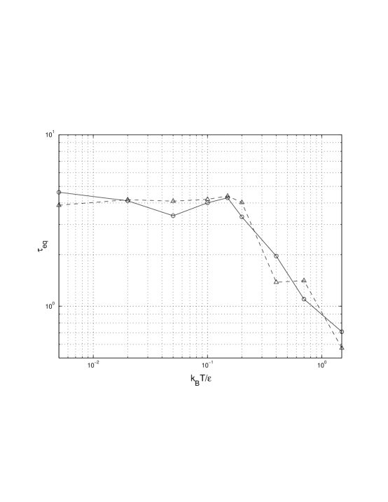
Figure 1: Calculated temperature dependence of the Compatible Monte Carlo energy relaxation time. The particle number density $\rho\cdot\sigma=0.2$. $\circ$ - 16 particles in the periodicity cell ( $L=80\cdot\sigma$, $M=32$); $\triangle$ - 256 particles in the periodicity cell ($L=1280\cdot\sigma$, $M=512$). The size of a subdomain was chosen to be $h_{1}=2.5\cdot\sigma$.

The temperature dependence of the relaxation time estimated in accordance with (17) is shown in Fig.1. In contrast to the ordinary Monte Carlo process the relaxation of CMC is not sensitive to the size of the periodicity domain and a fast equilibration implies that coarsening the particle number satisfies (in the case of the interaction potential (13) and, hence, in the high temperature limit (14) the requirements for the quality of the coarse variables set.

In the special case of the one-dimensional fluid, the main contribution to the distribution of the particle number $n_{i}^{k}$ at any lattice point is expected to come from its nearest neighbors. Therefore a simple possible form of the conditional probability table is given by:

$$P_{k}(n_{i}^{k},n_{j}^{k}\mid s^{1}_{ij},\ldots,s^{l}_{ij})=P_{k}(n_{i}^{k},n_{i+1}^{k}\mid n_{i-1}^{k},n_{i+2}^{k})$$ (18)

Quantities of $n_{i}^{k}$ were calculated at each lattice point $i$ for each produced configuration at the next finer level, and from them the probability distributions (18) were accumulated, forming the CP table. Then, multilevel Monte Carlo simulation was performed using this CP tables.

A suitable quantity for comparing simulation results at different levels is the fluctuation $\nu_{k}$ of the particle number in the subdomain of size $V^{k}$ (corresponding to the gridpoint of the lattice with meshsize $h_{k}=h_{1}\cdot 2^{k-1}$):

$$\nu_{k}=\frac{<n^{k^{2}}>-<n^{k}>^{2}}{<n^{k}>}$$ (19)

where the mean values are defined by probabilities $p_{k}(n)$ to display the particle number $n^{k}$ in a volume of size $V^{k}$: $<n^{k}>=\sum\limits_{n^{k}}n^{k}\cdot p_{k}(n^{k})$, $<n^{k^{2}}>=\sum\limits_{n^{k}}n^{k^{2}}\cdot p_{k}(n^{k})$.

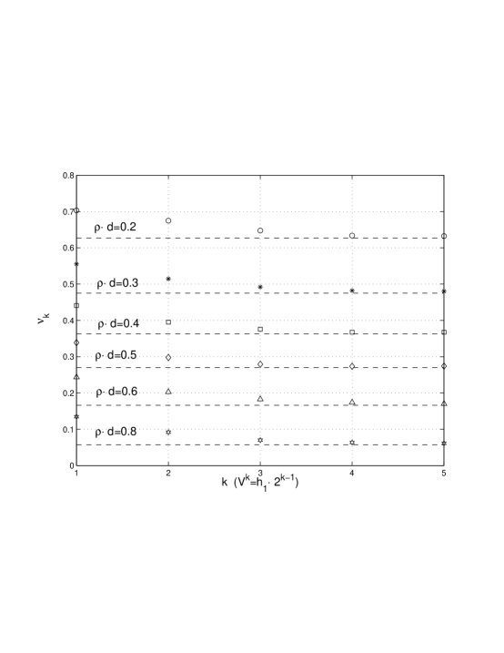
Figure 2: Particle number fluctuation at different levels (hard rods fluid, $h_{1}=2.5\cdot d$). Dashed lines correspond to exact bulk values (20).

The fluctuation of the particle number does not depend on the volume if it is sufficiently large (as compared with the correlation length) and is related with the isothermal compressibility $\kappa=\biggl{(}-\frac{1}{V}\frac{\partial V}{\partial P}\biggl{)}_{T={\it const}}$ [18]. For 1D hard core system the equation of state is found analytically (it is known as the Tonk’s equation [19]) and the isothermal compressibility is given by:

$$\nu_{\infty}=\rho\cdot k_{B}T\cdot\kappa=(1-\rho\cdot d)^{2}$$ (20)

Results of particle number fluctuation multilevel measurements in volumes of different sizes for hard rods systems are presented in Fig.2. The dependence of this quantity on the subdomain size is explained by the size effects and coincides with the expression of the grand canonical ensemble [14]:

$$\nu_{k}=\nu_{\infty}+\frac{C}{V^{k}}$$ (21)

where $\nu_{\infty}$ is the bulk value of the particle number fluctuation (20). The coefficient $C$ as well as $\nu_{\infty}$ depend on the particle number density. One can see from Fig.2 that at high temperatures (the interaction model (14) five levels are enough in order to achieve the bulk behavior in subdomains connected with gridpoints of the coarsest level.

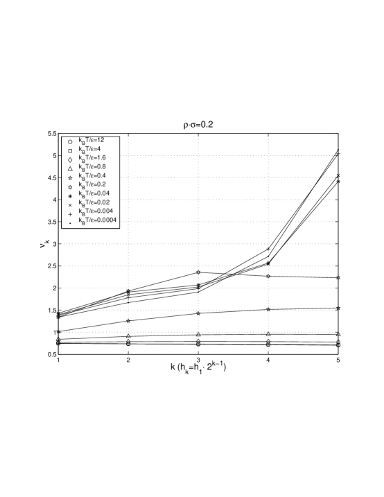
Figure 3: Particle number fluctuation at different levels (Lennard-Jones fluid, $h_{1}=2.5\cdot\sigma$).

In the case of the Lennard-Jones fluid the particle number fluctuations depends also on the temperature. The dependence on the meshsize (the subdomain volume) for system with the interaction potential (13) is shown in Fig.3 for different temperatures. One can see that at high temperatures the properties of the Lennard-Jones fluid are similar to the hard rods system (see Fig.2). At low temperatures the behavior of fluctuations drastically changes. The results obtained indicate that in contrast to the hard rods system the Lennard-Jones system loss homogeneity at low temperatures on fine scales.

4 CONCLUSION

It follows from the present results that in the framework of the multilevel Monte Carlo method a suitable choice of coarsening allows to attain the macroscopic behavior. The particle number fluctuation in subdomains of intermediate size tends to the exact value on increasingly coarser levels. The accuracy of averages (including the particle number fluctuation) depends only on the CP tables adequacy, which is achieved by the correct selection of the variable set.

The advantage of the multilevel Monte Carlo method consists in fast convergence of measured mean values due to the selfconsistent equilibration on different levels modes of wave lengths comparable with the simulation domain. The computational work on each level is proportional to the number of gridpoints and is independent of the particle number associated with the gridpoint. It leads to the high speed of the method as compared with conventional algorithms.

The equilibrium on fine levels (and in particular the frequency of the appearance of a given particle number in the simulation domain) is defined by the canonical ensemble configurations on coarsest level. The particle number in fine level simulation domains is variable and its distribution imitates the result of the grand canonical ensemble simulation [20]. The multilevel Monte Carlo method is not concerned with the equilibrium in accordance with the value of a chemical potential. It opens new way for the development of the one-phase approach to the phase-transition problem [21].

5 ACKNOWLEDGMENTS

The research has been supported by Israel Absorption Ministry, project No. 6682, by the U.S. Air Force Office of Scientific Research, contract No. F33615-97-D-5405, by the European Office of Aerospace Research and Development (EOARD) of the U.S. Air FORCE, contract No. F61775-00-WE067, by Israel Science Foundation Grant No. 696/97 and by the Carl F.Gauss Minerva Center for Scientific Computation at the Weizmann Institute of Science.

References

- [1] N.Metropolis, A.W.Rosenbluth, A.H.Teller, E.Teller, Equation of State Calculation by Fast Computing Machines, J. Chem. Phys., 21, 1087 (1953)
- [2] A.A.Maradudin, E.W.Montroll, O.H.Weiss, Theory of Lattice Dynamics in the Harmonic Approximation (Academic Press, New York and London, 1963).
- [3] M.P.Allen, D.J.Tildesley, Computer Simulation of Liquids (Oxford University Press, Oxford, 1987).
- [4] J.Yao, R.A.Greenkorn, K.C.Chao, Monte Carlo Simulation of the Grand Canonical Ensemble, Mol.Phys. 46, 587 (1982).
- [5] I.Ruff, A.Bararyai, G.Palinkas, K.Heinzinger, Grand Canonical Monte Carlo Simulation of Liquid Argon, J.Chem.Phys. 85, 2169 (1986).
- [6] G.R.Smith, A.D.Bruce, A Study of the Multi-Canonical Monte Carlo Method, J.Phys.A: Math. Gen. 28, 6623 (1995).
- [7] K.Binder, Applications of Monte Carlo Methods to Statistical Physics, Rep.Prog.Phys. 60, 487 (1997).
- [8] A.Z.Panagiotopoulos, Monte Carlo Methods for Phase Equilibria of Fluids, J.Phys.: Condens. Matter. 12, 25 (2000).
- [9] A.Brandt,The Gauss Center Research in Multiscale Scientific Computation: Six Year Summary, Gauss Center Report WI/GC-12, (1999) 74 p.
- [10] A.Brandt, Multigrid Methods in Lattice Field Computations, Nuclear Physics B26, 137 (1992).
- [11] A.Brandt, M.Galun, D.Ron, Optimal Multigrid Algorithms for Calculating Thermodynamic limits, J.Stat. Phys. 74, 313 (1993).
- [12] A.Brandt, Guide to multigrid development, in Multigrid Methods, edited by W.Hackbush and Trottenberg, Lecture Notes in Math. (Springer-Verlag, 1982), p.960
- [13] A.Brandt, D.Ron, Renormalization Multigrid (RMG): Coarse-to-fine Monte Carlo Acceleration and Optimal Derivation of Macroscopic Descriptions, in Multiscale Computational Methods in Chemistry and Physics, NATO Science Series, Computer and System Science, edited by A.Brandt, J.Bernholc and K.Binder, 177, IOS Press, Amsterdam (2000).
- [14] M.Rovere, D.W.Heerman, K.Binder, The Gas-Liquid Transition of the Two-Dimensional Lennard-Jones Fluid, J.Phys., 2, 7009 (1990).
- [15] H.Takahashi, A Simple Method for Treating the Statistical Mechanics of One-Dimensional Substances, Proc. Phys. Math. Soc. Jap., 24, 60 (1942).
- [16] Ya.I.Frenkel, Kinetic Theory of Liquids (Nauka, Leningrad, 1975)
- [17] E.Stoll, K.Binder, T.Schneider. Monte Carlo Investigation of the Two-Dimensional Kinetic Ising Model. Phys. Rev., B8, 3266 (1973).
- [18] T.L.Hill, Statistical Mechanics (Mc. Grow-Hill Book Company Inc., New-York-Toronto-London, 1956)
- [19] L.Tonks, The Complete Equation of State of One, Two and Three-Dimensional Gases of Hard Elastic Spheres, Phys. Rev, 50, 955 (1936).
- [20] A.Brandt, V.Ilyin, Multilevel Approach in Statistical Physics of Liquids, in Multiscale Computational Methods in Chemistry and Physics, NATO Science Series, Computer and System Science, edited by A.Brandt, J.Bernholc and K.Binder, 177, IOS Press, Amsterdam (2000).
- [21] G.A.Matynov, G.N.Sarkisov, Stability and Fist-Order Phase Transitions, Phys. Rev., B42, 2504 (1989).